Jul 15, 2010 - tinely fitting complex models to realistic spatial point pattern data. ... but more complex models, such as hierarchical models or models including ...
Submitted to the Annals of Applied Statistics arXiv: math.PR/0000000
A TOOLBOX FOR FITTING COMPLEX SPATIAL POINT PROCESS MODELS USING INTEGRATED NESTED LAPLACE APPROXIMATION (INLA) By Janine B. Illian, Centre for Research into Ecological and Environmental Modelling, University of St Andrews, Scotland and By Sigrunn H. Sørbye, Department of Mathematics and Statistics, University of Tromsø, Norway and By H˚ avard Rue Department of Mathematical Sciences, Norwegian University of Science and Technology, Trondheim, Norway This paper develops methodology that provides a toolbox for routinely fitting complex models to realistic spatial point pattern data. We consider models that are based on log-Gaussian Cox processes and include local interaction in these by considering constructed covariates. This enables us to use integrated nested Laplace approximation and to considerably speed up the inferential task. In addition, methods for model comparison and model assessment facilitate the modelling process. The performance of the approach is assessed in a simulation study. To demonstrate the versatility of the approach, models are fitted to two rather different examples, a large rainforest data set and a point pattern with multiple marks.
1. Introduction. These days a large variety of complex statistical models can be fitted routinely to complex data sets as a result of widely accessible high-level statistical software, such as R (R Development Core Team, 2009) or winbugs, (Lunn et al., 2000). For instance, the non-specialist user can estimate parameters in generalised linear mixed models or run a Gibbs sampler to fit a model in a Bayesian setting, and expert programming skills are no longer required. Researchers from many different disciplines are now able to analyse their data with sufficiently complex methods rather than resorting to simpler yet non-appropriate methods. In addition, methods for the assessment of a model’s fit as well as for the comparison of different models are widely used in practical applications. The routine fitting of spatial point process models to (complex) data sets, however, is still in its infancy. This is despite a rapidly improving technology that facilitates data collection, and a growing awareness of the importance and relevance of small-scale spatial information. Spatially explicit data sets have become increasingly available in many areas of science, including plant ecology (Burslem et al., 2001; Law et al., 2001), animal ecology (Forchhammer and Boomsma, 1995, 1998), geosciences (Naylor et al., 2009; Ogata, 1999), molecular genetics (Hardy and Vekemans, 2002), evolution (Johnson and Boerlijst, 2002) and game theory (Killingback and Doebeli, 1996) with the aim of answering a similarly broad range of scientific questions. Currently, these data sets are often analysed with methods that do not make full use of the available spatially explicit information. Hence there is a need for making the existing point process methodology available to applied scientists by facilitating the fitting of suitable models to help provide answers to concrete scientific questions. There have been previous advances in facilitating routine model fitting for spatial Gibbs point processes, which model local spatial interaction in point patterns. Most markedly, the work by Baddeley and AMS 2000 subject classifications: Primary 60K35, 60K35; secondary 60K35 Keywords and phrases: Cox processes, marked point patterns, model assessment, model comparison
1 imsart-aoas ver. 2010/04/27 file: Illian_Soerbye_Rue.tex date: July 15, 2010
2
Turner (2000) has facilitated the routine fitting of Gibbs point processes based on an approximation of the pseudolikelihood to avoid the issue of intractable normalising constants (Berman and Turner, 1992; Lawson, 1992) as well as the approximate likelihood approach by Huang and Ogata Huang and Ogata (1999). Work by Baddeley et al. (2005) and Stoyan and Grabarnik (1991) has provided methods for model assessment for some Gibbs processes. Many of these have been made readily available through the library spatstat for R (Baddeley and Turner, 2005). However, most Gibbs process models considered in the literature are relatively simple. In an attempt to generalise the approach in Baddeley and Turner (2005), Illian and Hendrichsen (2010) include random effects in Gibbs point processes but more complex models, such as hierarchical models or models including quantitative marks, currently cannot be fitted in this framework. Similarly, methods for model comparison or assessment considered in Baddeley et al. (2005) and Stoyan and Grabarnik (1991) are restricted to relatively simple models. Furthermore, both estimation based on maximum likelihood and that based on pseudolikelihood are approximate so that inference is not straight forward. The approximations become less reliable with increasing interaction strength (Baddeley and Turner, 2000). Cox processes are another, particularly flexible, class of spatial point process models (Møller and Waagepetersen, 2007). Even though many theoretical results have been discussed in the literature for these (Møller and Waagepetersen, 2004), the practical fitting of Cox point process models to point pattern data remains difficult due to intractable likelihoods. Fitting a Cox process to data is typically based on Markov chain Monte Carlo (MCMC) methods. These require expert programming skills and can be very time-consuming both to tune and to run (Møller and Waagepetersen, 2004) so that fitting complex models can easily become computationally prohibitive. Methods for model comparison or model assessment for Cox processes have not been discussed in the literature and there have been no attempts at providing routine model fitting approaches for these processes. To the authors’ knowledge, Cox processes have not been used outside the statistical literature to answer concrete scientific questions. Realistically complex data sets often consist of the exact spatial locations of the objects or events of interest, as well as of further information on these objects, i.e. marks. They are often more complex than the classical data sets that have been analysed with point process methodology in the past. For example, some of these data sets consist of a large number of points representing the locations of objects in space (Burslem et al., 2001). The data often contain further information on the properties of the objects, i.e. on several potentially dependent qualitative as well as quantitative marks (Moore et al., 2010). Frequently, several (spatial) covariates have been collected so that there is an interest in deciding which of these are relevant (John et al., 2007). Currently, Cox process models have not been fitted to data sets of such complexity. Applied researchers are aware that spatial behaviour tends to vary at a number of spatial scales as a result of different underlying mechanisms that drive the pattern (Wiegand et al., 2007; Latimer et al., 2009). Local spatial behaviour is often of specific interest but the spatial structure also varies on a larger spatial scale due to the influence of observed or unobserved spatial covariates. Cox processes model spatial patterns relative to observed or unobserved spatial trends and would be ideal models for these data sets. In particular, assuming a stochastic spatial trend makes them particularly realistic and relevant in applications. However, two main issues arise: (i) the Cox process models that have been considered so far are not complex enough to be suitable for many realistic data sets, and (ii) they typically do not consider spatial structures at different spatial scales within the same model. More specifically, regarding the first issue, most applications of Cox process models have focused on the analysis of relatively small spatial patterns in terms of the locations of individual species. Very few attempts have been made at fitting models to both the pattern and the marks, in particular not to patterns with multiple dependent continuous marks (Ho and Stoyan, 2008; Myllym¨aki and Penttinen, 2009). As far as the second issue is concerned, a specific strength of spatial point process models is their ability to take into account detailed information at very small spatial scales contained in spatial point
imsart-aoas ver. 2010/04/27 file: Illian_Soerbye_Rue.tex date: July 15, 2010
FITTING COMPLEX SPATIAL POINT PROCESS MODELS WITH INLA
3
pattern data, in terms of the local structure formed by an individual and its neighbours. So far, Cox processes have often been used to relate the locations of individuals to environmental variation, phenomena that typically operate on larger spatial scales. However, different mechanisms operate at a smaller spatial scale. Spatial point data sets are often collected with a specific interest in the local behaviour of individuals, such as spatial interaction or local clustering (Law et al., 2001; Latimer et al., 2009). In this paper, we aim at proposing solutions to both these issues. The approach that we suggest here allows very general (hierarchical) models to be fitted including models of both the spatial pattern and associated marks. Using a Bayesian approach, we provide modern model fitting methodology for complex spatial point pattern data similar to what is common in other areas of statistics and has become a standard in many areas of application, including methods for model comparison and validation. We introduce a general modelling framework that provides a toolbox enabling the routine fitting of models to realistically complex data sets. The approach is based on integrated nested Laplace approximation (INLA) (Rue et al., 2009) which speeds up parameter estimation substantially so that Cox processes can be fitted within feasible time. In order to make the methods accessible to non-specialists, an R package that may be used to run INLA is available and contains generic functions for fitting spatial point process models, see http://www.r-inla.org/. In addition, we suggest an approach to fitting Cox process models that reflect both the local spatial structure and spatial behaviour at a larger spatial scale by using constructed covariates that account for spatial behaviour at different spatial scales. In doing this, we avoid issues with intractable normalising constants common in Gibbs process models and are able to consider local spatial structures within the flexible class of Cox processes. This paper is structured as follows. The general methodology is introduced in Section . In Section 3 we investigate the idea of mimicking local spatial behaviour by using constructed covariates in a simulation study in the context of (artificial) data with known spatial structures and inspect patterns resulting from the fitted models. Section 4 discusses a model for a large data set with both observed and constructed covariates and fits this to a rainforest data set. A hierarchical approach is considered in Section 5, where both (multiple) marks and the underlying pattern in a complex data set are modelled. 2. Methods. 2.1. Spatial point process models. Spatial point processes have been discussed in detail in the literature, see Stoyan et al. (1995), van Lieshout (2000), Diggle (2003), Møller and Waagepetersen (2004) and Illian et al. (2008) for details. Here we aim at modelling a spatial point pattern x = (ξ1 , . . . , ξn ), regarding it as a realisation from a spatial point process X. For simplicity we consider only point processes in R2 but the approaches can be generalised to point patterns in higher dimensions. We refer the reader to the literature for more details about different (classes of) spatial point process models such as the simple Poisson process, the standard null model of complete spatial randomness, as well as the rich class of Gibbs (or Markov) processes (van Lieshout, 2000). Here, we discuss the class of Cox processes, in particular log-Gaussian Cox processes. Cox processes lend themselves well to modelling spatial point pattern data with spatially varying environmental conditions (Møller and Waagepetersen, 2007) as they model spatial patterns based on an underlying (or latent) random field Λ(·) that describes the random intensity, assuming independence given this field. In other words, given the random field, the point pattern forms a Poisson process. Log-Gaussian Cox processes as considered for example in Møller et al. (1998) and Møller and Waagepetersen (2004, 2007), are a particularly flexible class, where Λ(s) has the form Λ(s) = exp{Z(s)}, and {Z(s)} is a Gaussian random field, s ∈ R2 . Other examples of Cox processes include shot-noise Cox processes (Møller and Waagepetersen, 2004). Here, we consider a general class of spatial point process models based on log-Gaussian Cox processes that admits both small and larger scale spatial behaviour. In order to do so, we employ constructed covariates reflecting the spatial structure contained in the spatial pattern to take into account behaviour
imsart-aoas ver. 2010/04/27 file: Illian_Soerbye_Rue.tex date: July 15, 2010
4
at different spatial resolutions. This allows us to consider models with local interaction as latent Gaussian models and hence to use INLA for parameter estimation and model fitting. 2.2. Integrated nested Laplace approximation (INLA). Cox processes are a special case of the very general class of latent Gaussian models, models of an outcome variable yi that assume independence conditional on some underlying latent field ζ and hyperparameters θj , j = 1, . . . , J. Rue et al. (2009) show that if ζ has a sparse precision matrix and the number of hyperparameters is small (i.e. ≤ 7), inference based on integrated nested Laplace approximation (INLA) is fast. The main aim of the INLA approach is to approximate the posteriors of interest, i.e. the marginal posteriors for the latent field π(ζi |y), and the marginal posteriors for the hyperparameters π(θj |y), and use these to calculate posterior means, variances etc. These posteriors can be written as Z
(2.1)
π(ζi |y) =
π(ζi |θ, y)π(θ|y)dθ Z
(2.2)
π(θj |y) =
π(θ|y)dθ−j .
The nested formulation is used to compute π(ζi |y) by approximating π(ζi |θ, y) and π(θ|y), and then to use numerical integration to integrate out θ. This is feasible, since the dimension of θ is small. Similarly, π(θj |y) is calculated by approximating π(θ|y) and integrating out θ−j . The marginal posterior in equations (2.1) and (2.2) can be calculated using the Laplace approximation ¯
π(ζ, θ, y) ¯¯ π ˜ (θ|y) ∝ π ˜G (ζ|θ, y) ¯ζ=ζ ∗ (θ) where π ˜G (ζ|θ, y) is the Gaussian approximation to the full conditional of ζ, and ζ ∗ (θ) is the mode of the full conditional for ζ, for a given θ. This makes sense, since the full conditional of a zero mean Gauss Markov random field can often be well approximated by a Gaussian distribution by matching the mode and the curvature at the mode (Rue and Held, 2005). Rue et al. (2009) show that this fact and the nested approach yield a very accurate approximation if applied to latent Gaussian models. As a result, the time required for fitting these models is substantially reduced. 2.3. Log-Gaussian Cox processes with local spatial structures. The class of latent Gaussian models comprises log-Gaussian Cox processes and hence the INLA approach may be applied to fit these. Specifically, the observation window is discretised into N = nrow × ncol grid cells {sij }, each with area |sij |, i = 1, . . . , nrow , j = 1, . . . , ncol . The points in the pattern can then be described by {ξijkij } with kij = 1, . . . , yij , where yij denotes the observed number of points in grid cell sij . We condition on the point pattern and conditionally on ηij = Z(sij ) we have (2.3)
yij |ηij ∼ P o(|sij | exp(ηij )),
see Rue et al. (2009). In this paper we generalise an approach in Rue et al. (2009) by incorporating local spatial behaviour into the models based on constructed covariates and considering more complex models. Constructed covariates are summary characteristics defined for any location in the observation window reflecting inter-individual spatial behaviour such as local interaction or competition. We assume that this behaviour operates at a smaller spatial scale than spatial aggregation due to (observed or unobserved) spatial covariates. The use of constructed covariates yields models with local spatial interaction within the flexible class of log-Gaussian Cox process models. It avoids issues with intractable normalising constants that are common in the context of Gibbs processes (Møller and Waagepetersen, 2004), since the covariates operate directly on the intensity of the pattern rather than on the density or the conditional intensity (Schoenberg, 2005). imsart-aoas ver. 2010/04/27 file: Illian_Soerbye_Rue.tex date: July 15, 2010
FITTING COMPLEX SPATIAL POINT PROCESS MODELS WITH INLA
5
We model ηij as (2.4)
ηij = β0 + β1 z1 (sij ) + . . . + βp zp (sij ) + f (zc (sij )) + fs (sij ) + uij ,
where z1 (sij ), . . . , zp (sij ) are (empirical) spatial covariates and zc (sij ) denotes a constructed covariate. The functional relationship between the outcome variable and the constructed covariate is typically not obvious and might often not be linear. We thus estimate this relationship explicitly by a smooth function f (zc (sij )) and inspect this estimate to gain further information on the form of the spatial dependence. In the examples In Sections 4 and 5 follow, this function will be modelled as a first-order random walk, constrained to sum to zero. The function fs (sij ) is a spatially structured effect that reflects large scale spatial variation in the pattern not captured by the covariates. This effect will be modelled using a second-order random walk on a lattice, using vague gamma priors for the hyperparameter and constrained to sum to zero (Rue and Held, 2005). uij denotes a spatially unstructured i.i.d. error term with uij ∼ N (0, 1). The constructed covariate considered in this paper is based on nearest point distance. Specifically, for the mid-points of each grid cell we find the distance to the nearest point in the pattern as (2.5)
zc (sij ) = d(sij ) = min(kcij − ξl k), ξl ∈x
where cij denotes the centre point of cell sij and k · k denotes the Euclidean distance. This covariate is simple and fast to compute and it performs well in both the simulation study in Section as well as with the real examples considered in Section 4 and 5. During the modelling process, methods for model comparison based on the deviance information criterion (DIC) (Spiegelhalter et al., 2002), may be used to compare different models with different levels of complexity. Furthermore, the (estimated) error field in (2.4) may be assessed once the model has been fitted and interpreted as a spatial residual. This provides a method for model assessment akin to residuals in linear models since remaining spatial structures in the estimated error term reveal spatial behaviour that has not been captured by the model. This approach yields a toolbox for fitting, comparing and assessing realistically complex models of spatial point pattern data. We show that different types of flexible models can be fitted to point pattern data with complex structures with the INLA approach within reasonable computation time. This includes large point patterns with covariates operating on a large spatial scale and local clustering (Section 4) as well as point pattern data with several dependent marks which also depend on the intensity of the pattern (Section 5). 3. Using constructed covariates to account for local spatial structure – a simulation study. In Sections 4 and 5 we use a constructed covariate primarily to incorporate local spatial structure into a model, while accounting for spatial variation at a larger spatial scale. To illustrate the use of the given constructed covariate and to assess the performance of the resulting models, we simulate point patterns from various classical point-process models. Note, however, that we do not aim at explicitly estimating the parameters of these models but at assessing (i) whether known spatial structures may be detected through the use of the constructed covariate, as suggested here, and (ii) whether simulations from the fitted models generate patterns with similar characteristics. In the applications we have in mind, such as those discussed in the examples in Sections and , the data structure is typically more complicated. For the purpose of this simulation study we consider three different situations: patterns with local repulsion (Section 3.1), patterns with local clustering (Section 3.2) and patterns with local clustering in the presence of a larger-scale spatial trend (Section 3.3). We generate example patterns from different point process models with these properties. In order to use INLA to fit models to these patterns, the unit square is discretised as discussed in Section 2.3 using a 100 × 100 grid. imsart-aoas ver. 2010/04/27 file: Illian_Soerbye_Rue.tex date: July 15, 2010
6
In Sections 3.1 and 3.2 we initially assume that there is no large-scale spatial variation, with the aim of inspecting only the constructed covariate and we consider (3.1)
ηij = β0 + f (zc (sij )),
using the notation in Section 2.3. In Section 3.3 we consider both small- and large-scale spatial structures by including a spatially structured effect fs (sij ) in addition to the constructed covariate zc (sij ) and (3.2)
ηij = β0 + f (zc (sij )) + fs (sij ).
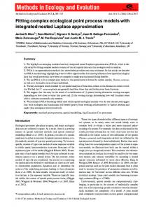
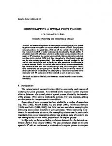
We evaluate the fitted models by applying the Metropolis–Hastings algorithm (Metropolis et al., 1953; Hastings, 1970) to simulate patterns from these models and then compare characteristics of the simulated patterns with the generated example patterns. The simulated patterns in Sections 3.1 to 3.3 each result from 100,000 iterations of the algorithm, where the initial patterns consist of the same number of points as the generated example patterns, randomly scattered in the unit square. 3.1. Modelling repulsion. To inspect the performance of constructed covariates for repulsion, we generate a pattern from a homogeneous Strauss process (Strauss, 1975) on the unit square, with medium repulsion β = 700 (intensity parameter), γ = 0.5 (interaction parameter) and interaction radius r = 0.05 (Figure 1 (a)). We then fit a model to the pattern as in equation (3.1) using the constructed covariate in (2.5) (Figure 1 (b)). The shape of the estimated functional relationship between the constructed covariate and the outcome variable (Figure 1 (c)) indicates that at small values of the covariate the intensity is positively related to the constructed covariate, clearly reflecting repulsion. At larger distances (> 0.05) the function levels out distinctly, indicating that beyond these distances the covariate and the intensity are unrelated, i.e. the spatial pattern shows random behaviour. In other words, the functional relationship not only characterises the pattern as regular but also correctly identifies the interaction distance as 0.05. The pattern resulting from the Metropolis–Hastings algorithm (Figure 1 (d)) shows very similar characteristics to those in the original pattern. This indicates that the model based on the nearest point constructed covariate in equation (2.5) captures adequately the spatial information contained in the repulsive pattern. The estimated pair-correlation functions for the simulated and the original pattern confirm this, as they look very similar (Figure 1 (e)). 3.2. Modelling clustering. In order to assess the performance of the model in (3.1) in the context of clustered patterns, we generate a pattern from a homogeneous Thomas process (Neyman and Scott, 1952) in the unit square, with parameters κ = 10 (the intensity of the Poisson process of cluster centres), σ = 0.05 (the standard deviation of the distance of a process point from the cluster centre) and µ = 50 (the expected number of points per cluster) (Figure 2 (a)). We fit the model in equation (3.1), again using the constructed covariate in (2.5) (Figure 2 (b)). The shape of the estimated functional relationship between the constructed covariate and the outcome variable (Figure 2 (c)) indicates clearly that the intensity is negatively related to the constructed covariate at small values of the covariate reflecting clustering at smaller distances. At larger distances (> 0.1) the function levels out, indicating that at these distances the covariate and the intensity are unrelated. The pattern simulated from the fitted model (Figure 2 (d)) shows that the constructed covariate introduces some clustering in the model. However, the resulting pattern shows fewer and less distinct clusters than the original pattern. Similarly, the estimated pair-correlation function for pattern simulated from the fitted model shows a weaker local clustering effect than the original pattern (Figure 2 (e)). 3.3. Modelling small scale clustering in the presence of large-scale inhomogeneity. So far, we have considered constructed covariates only for patterns with local interaction (or clustering) to illustrate their use. In applications, however, including those we discuss below, different mechanisms operate at imsart-aoas ver. 2010/04/27 file: Illian_Soerbye_Rue.tex date: July 15, 2010
7
1.0
1.0
1.0
FITTING COMPLEX SPATIAL POINT PROCESS MODELS WITH INLA
0.5
0.10
0.0 −0.5
0.02
0.02
0.0
0.0
0.04
−1.0
0.06
0.5
0.5
0.08
0.0
0.5
1.0
0.0
0.5
0.06
0.08
0.10
(b)
(c)
0.0
0.5
1.0
1.5
2.0
0.5
2.5
3.0
3.5
1.0
4.0
(a)
0.04
1.0
0.00
0.0
0.5
(d)
0.05
0.10
0.15
0.20
0.25
1.0
(e)
Fig 1. Simulated Strauss process with medium repulsion (r = 0.05, β = 700, γ = 0.05) (a), the associated constructed covariate for this pattern (b), the estimated functional relationship between the outcome and the constructed covariate (c), a pattern simulated from the fitted model after 100,000 iterations (d) and the estimated pair correlation function for the original (solid line) and simulated pattern (dashed line) (e).
different spatial scales. Patterns may be locally clustered, e.g. due to dispersal mechanisms, but may also show aggregation at a larger spatial scale, e.g. due to dependence on underlying observed or unobserved covariates. Hence the main reason for using constructed covariates in the real examples in Sections 4 and 5 is to distinguish behaviour at different spatial resolutions, in order to provide information on mechanisms operating at different spatial scales. We illustrate the use of constructed covariates in this context by generating an inhomogeneous, locally clustered pattern mimicking a situation where different mechanisms have caused the local clustering and the large scale inhomogeneity. In applications, the inhomogeneity may be modelled using suitable spatially varying covariates or assuming an unobserved spatial variation. We generate a pattern from an inhomogeneous Thomas process with parameters σ = 0.01 and µ = 5 and a simple trend function for the intensity of parent points given by κ(x1 , x2 ) = 50x1 . This process is superimposed with a pattern generated from an inhomogeneous Poisson process with trend function λ = x1 /4 (Figure 3 (a)). We again use the constructed covariate based on nearest-point distance (2.5), see Figure 3 (b), and fit the model in equation (3.2). The inspection of the functional relationship between the constructed covariate and the outcome (Figure 3 (c)) shows that at small values of the covariate the intensity is negatively related to the constructed covariate, reflecting clustering at smaller distances. Patterns simulated from the fitted model look similar to the original pattern (Figure 3 (d)) and the estimated spatially structured effect picks up the larger-scale spatial behaviour (Figure 3 (e)). However, local clustering is slightly stronger in the original pattern than in the simulated pattern (Figure 3 (f)). 3.4. Discussion on constructed covariates. With the aim of assessing the performance of models with constructed covariates reflecting small scale inter-individual spatial behaviour, we consider a number imsart-aoas ver. 2010/04/27 file: Illian_Soerbye_Rue.tex date: July 15, 2010
6
1.0
1.0
8
4
0.25
0.5
0.5
2
0.20
0
0.15
−2
0.10
0.00
0.0
0.0
0.05
0.0
0.5
1.0
0.0
0.5
0.10
0.15
0.20
0.25
0.30
(b)
(c)
0.0
0
2
4
6
0.5
8
10
12
1.0
(a)
0.05
1.0
0.00
0.0
0.5
(d)
0.05
0.10
0.15
0.20
0.25
1.0
(e)
Fig 2. Simulated Thomas process with parameters κ = 10, σ = 0.05 and µ = 50 (a), the associated constructed covariate for this pattern (b), the estimated functional relationship between the outcome and the constructed covariate (c), a pattern simulated from the fitted model after 100000 iterations (d) and the estimated pair correlation function for the original (solid line) and simulated pattern (dashed line) (e).
of simulated point patterns for three different scenarios: repulsion, clustering and small-scale clustering in the presence of large scale inhomogeneity. In all cases the local spatial structure can be clearly identified. The given constructed covariate does not only take account of local spatial structures but also characterises the spatial behaviour. The functional form of the dependence of the intensity on the constructed covariate clearly reflects the character of the local behaviour. This section presents only a small part of an extensive simulation study; the results shown here are typical examples. We have run simulations from the same models as above with different sets of parameters and have obtained essentially the same results. Further, fitting the model in equation (3.1) to patterns simulated from a homogeneous Poisson process resulted in a non-significant functional relationship, i.e. the modelling approach does not pick up spurious clustering or regularity. The approach allows us to fit models that take into account small-scale spatial behaviour, regularity as well as clustering, in the context of log-Gaussian Cox processes, i.e. as latent Gaussian models. Since these can be fitted using the INLA approach, fitting is fast and exact. In addition, we avoid some of the typical problems that arise with Gibbs process models, i.e. we do not face issues of intractable normalising constants, and regular as well clustered patterns may be modelled. Certainly, the constructed covariate in equation (2.5) that we consider here is not the only possible choice. A covariate based on distance to the nearest point is likely to be rather ”short-sighted”, so that other constructed covariates might be more suitable for detecting specific spatial structures. In particular, taking into account these limitations, it is not surprising that patterns simulated from models based on d show less clustering than the original data. Clearly, a more general covariate such as the distance to the kth nearest point may be used. Other covariates, such as the local intensity or the number imsart-aoas ver. 2010/04/27 file: Illian_Soerbye_Rue.tex date: July 15, 2010
9
1
0.20
2
3
1.0
1.0
FITTING COMPLEX SPATIAL POINT PROCESS MODELS WITH INLA
0
0.05
0.0
0.0
0.05
−1
0.10
−2
0.5
0.5
0.15
0.5
1.0
0.0
0.10
0.15
0.20
1.0
(b)
(c) 1.5
25
1.0
1.0
(a)
0.5
20
1.0
−1.0
15 10
−0.5
5
0.0
0.5
0.5
0.5
0.00
0.0
0.0
0
−1.5
0.0
0.5
(d)
1.0
0.0
0.5
(e)
0.05
0.10
0.15
0.20
0.25
1.0
(f)
Fig 3. Realisation of an inhomogeneous Thomas process with parameters σ = 0.01, µ = 5 and trend function κ(x1 , x2 ) = 50x1 superimposed on an inhomogeneous Poisson process with trend function λ = x1 /4 (a), the associated constructed covariate for this pattern (b), the estimated functional relationship between the outcome and the constructed covariate (c), a pattern simulated from the fitted model after 100000 iterations (d), the estimated spatially structured effect (e) and the estimated pair correlation function for the original (solid line) and the simulated (dashed line) pattern (f ).
of points within a fixed interaction radius from a location s ∈ R2 are certainly also suitable. A nice property of the given constructed covariate based on nearest- point distance is that it is parameter-free. For this reason, it is not necessary to choose explicitly the resolution of the local spatial behaviour, e.g. as an interaction radius. Also, note that since the distance to the nearest point in point pattern x for a location s ∈ R may be interpreted as a graph associated with x ∪ {s}, other constructed covariates based on different types of graphs (Rajala and Illian, 2010) may also be used as constructed covariates. Similarly, an approach based on morphological functions may be used for this purpose. Note that one could also consider constructed marks based on first or second order summary characteristics (Illian et al., 2008) that are defined only for the points in the pattern and include these in the model. Distinguishing spatial behaviour at different spatial scales is clearly an ill-posed problem, since the behaviour at one spatial scale is not independent of that at different spatial scales (Diggle, 2003). The approach we take here will not always be able to distinguish clustering at different scales. However, different mechanisms that operate at very similar spatial scales are likely to be non-identifiable by any method, irrespective of the choice of model or the constructed covariate. Admittedly, the use of constructed covariates is of a rather subjective nature. Clearly, in applications the covariates have to be constructed carefully, depending on the questions of interest; different types of constructed covariates may be suitable in different contexts. However, similarly subjective decisions are usually made when a model is fitted that is purely based on empirical covariates, as these have been specifically chosen as potentially influencing the outcome variable, based on background knowledge. 4. Large point patterns with environmental covariates and local interaction. imsart-aoas ver. 2010/04/27 file: Illian_Soerbye_Rue.tex date: July 15, 2010
10
4.1. Modelling approach. In order to illustrate our modelling approach and, in particular, the use of constructed covariates in practice, we consider a point pattern x = (ξ1 , . . . , ξn ), where the number of points n is potentially very large. The aim is to fit the model in equation (2.4) to x, i.e. the point pattern is assumed to depend on one or several (observed or unobserved) environmental covariates z1 , . . . , zp . In addition to the empirical covariates, which are likely to have an impact on the larger scale spatial behaviour, we again use a constructed covariate to account for local clustering. In the application we have in mind (see Section 4.2) this clustering is a result of locally operating seed-dispersal mechanisms. Here we extend previous approaches to modelling these data with a Cox process (Rue et al., 2009) by using constructed covariates to reflect local clustering. The spatially structured term in (2.4) is included to capture behaviour at spatial scales not accounted for by the covariates. The spatially unstructered effect or the error field in (2.4) is used to detect any remaining spatial structures in the model and may be interpreted as a spatial residual term, as noted above. 4.2. Application to example data set. 4.2.1. The rainforest data. Some extraordinarily detailed multi-species maps are being collected in tropical forests as part of an international effort to gain greater understanding of these ecosystems (Condit, 1998; Hubbell et al., 1999; Burslem et al., 2001; Hubbell et al., 2005). These data comprise the locations of all trees with diameters at breast height (dbh) 1 cm or greater, a measure of the size of the trees (dbh), and the species identity of the trees. The data usually amount to several hundred thousand trees in large (25 ha or 50 ha) plots that have not been subject to any sustained disturbance such as logging. The spatial distribution of these trees is likely to be determined by both spatially varying environmental conditions and local dispersal. Recently, spatial point process methodology has been applied to analyse some of these data sets (Law et al., 2009; Wiegand et al., 2007) using non-parametric descriptive methods. In addition, there have been some explicit modelling attempts, including Waagepetersen (2007) and Waagepetersen and Guan (2009). Rue et al. (2009) model the spatial pattern formed by a tropical rain forest tree species solely on the underlying environmental conditions and use the INLA approach to fit the model. We analyse the same data here. Since the spatial structure in a forest also reflects dispersal mechanisms, we include a constructed covariate to account for local clustering. Figure 4 shows the spatial pattern formed by a total of 3887 trees of the species Beilschmiedia pendula Lauraceae on Barro Colorado Island (BCI). For the given data set, we apply the model ηij = β0 + β1 · z1ij + β2 · z2ij + f (zc (sij )) + fs (sij ) + uij , where the observed covariates z1ij and z2ij are normalised elevation and gradient for each grid cell (Figure 5 (a) and (b)); f (zc (sij )) is a function of the constructed covariate (2.5) (Figure 5 (c)). 4.2.2. Results. The parameter estimates of the fixed effects in the model are β1 = 0.157 and β2 = 0.088. These results indicate that trees are more likely to be located in areas where the two environmental covariates have high values. However, only the effect of the second covariate (gradient) is significant as the 95% posterior interval (0.014, 0.163) does not cover 0. The effect of the first covariate (elevation) is not significant, having a posterior interval equal to (−0.059, 0.373). The plot of the constructed covariate in Figure 5 (d) illustrates that a significant local clustering effect has been identified by the model. The structured spatial effect (Figure 5 (e)) clearly accounts for spatial behaviour at a scale larger than that reflected in the constructed covariate. However, a residual spatial structure is visible in Figure 5 (f), indicating that the model does not sufficiently explain all the spatial structure contained in the data. This might be due to further covariates that operate at different spatial scales than the structured effect and the covariates that have been considered. Clearly, the residual plot indicates that the current model appears to be unable to account for the complete absence of Beilschmidia trees in the central area (Figure 4). imsart-aoas ver. 2010/04/27 file: Illian_Soerbye_Rue.tex date: July 15, 2010
11
0
250
500
FITTING COMPLEX SPATIAL POINT PROCESS MODELS WITH INLA
0
500
1000
Fig 4. Spatial pattern of the species Beilschmiedia pendula Lauraceae on Barro Colorado Island, Panama. 15 10 5 0 −5 −10 −15 −20
(b)
100 80 60 40 20
(c)
10
(a)
0.20 0.15 0.10 0.05 0.00 −0.05
1.0
5
2.0 1.5
0.5
0
1.0 0.5
−5
0.0
0.0
0
20
40
60
(d)
80
−0.5
100
(e)
−0.5
(f)
Fig 5. Top panels: The normalised covariates elevation (a) and gradient (b) and the constructed covariate (c) reflecting local clustering for the rain forest data. Bottom panels: The estimated function of the constructed covariate (d), the estimated spatial structured (e) and unstructured effect (f ).
4.3. Discussion on rainforest data. In this section, we consider a Cox process model for a point pattern data set with a large number of points and two observed covariates. Waagepetersen (2007) and Waagepetersen and Guan (2009) model the patterns formed by rainforest tree species with this data structure, using Thomas processes to include local clustering resulting from seed dispersal. This approximate approach is based on the minimum contrast method for parameter estimation. Rue et al. (2009) consider the same data in the context of Cox processes to demonstrate that log-Gaussian Cox processes can be fitted conveniently to a large spatial point pattern using INLA solely on basis of the environmental covariates. We generalise this approach and fit a model based on the two empirical covariates and a constructed covariate that reflects local clustering as a result of local seed dispersal, as discussed above. imsart-aoas ver. 2010/04/27 file: Illian_Soerbye_Rue.tex date: July 15, 2010
12
The approach accommodates model comparison and model assessment, both of which are of practical value in many applications. In particular, fitting the model took less than 30 minutes on a standard PC. When further covariates are available it is thus straightforward to fit the model repeatedly with different sets of empirical covariates and model comparison may be done based on the DIC. An inspection of the error field indicates that some spatial structure still remains in the data which cannot be explained by the current model, i.e. the current model can still be improved on. It is not surprising to see that the pattern exhibits spatial dependence at a number of spatial scales, in particular given the size of the pattern. The remaining spatial structures possibly operate at different spatial scales than the structured spatial effect and the covariates considered. Including further covariates that operate at intermediate spatial scales, e.g. data on soil properties might improve the model. Previous approaches to fitting a model to these data (Waagepetersen, 2007; Waagepetersen and Guan, 2009) have not been able to reveal the shortcomings of their models. The approach discussed here can be extended easily to allow more complex models to be fitted, including models with larger number of environmental covariates or a model of both the spatial pattern and associated marks, along the lines of the model discussed in Section 5. For instance, this may include a model of both the spatial pattern and the size or the growth of the trees. 5. Modelling marks and pattern in a marked point pattern with multiple marks. Modelling the behaviour of individuals in space based simply on the individuals’ location and ignoring their properties is certainly a gross over-simplification for many systems. In practice, researchers hence often collect data on the locations of the individuals along with data on additional properties, i.e. marks. In this section we discuss a marked point pattern with several dependent marks, which also depend on the spatial pattern, and consider a joint model of the marks and the pattern. Models where marks depend on the point pattern have recently been considered in the literature (Menezes, 2005; Ho and Stoyan, 2008; Myllym¨aki and Penttinen, 2009). Also note the work by Diggle et al. (2010), where a point process with intensity dependent marks is used in the context of preferential sampling in geostatistics. The model we fit here is more general than these related models, since we take into account additionally local spatial structures through a constructed covariate and model multiple marks. 5.1. Data structure and modelling approach. We analyse a spatial point pattern x = (ξ1 , . . . , ξn ) together with several types of nonindependent associated marks. We consider only two marks m1 = (m11 , . . . , m1n ) and m2 = (m21 , . . . , m2n ) here but the approach can be generalised in a straightforward way to include more than two marks. The m1 are assumed to follow an exponential family distribution F1θ1 with parameter vector θ1 = (θ11 , . . . , θ1q ) and to depend on the intensity of the point pattern, while the m2 are assumed to follow a (different) exponential family distribution F2θ2 with parameter vector θ2 = (θ21 , . . . , θ2q ) and to depend both on the intensity of the point pattern but and on the marks m1 . Without loss of generality, the parameters θ11 and θ21 are the location parameters of the distributions F1 and F2 , respectively. We discretise the observation window as discussed in Section 2.3, and for the spatial pattern we assume the model (5.1)
ηij = β01 + β1 · fs (sij ) + f (zc (sij )) + uij ,
using the same notation as in (2.4). For the marks, we construct a model where the marks m1 depend on the pattern by assuming that they depend on the same spatially structured effect fs (sij ). Specifically, we assume that m1 (ξijkij )|κijkij ∼ F1θ1 (κijkij , θ12 , . . . , θ1q ) with (5.2)
κijkij = β02 + β2 · fs (sij ) + vijkij ,
where vijkij is another error term. The marks m2 are assumed to depend both on the spatial pattern through fs (sij ) and on the marks m1 . We thus have that m2 (ξijkij )|νijkij ∼ F2θ2 (νijkij , θ22 , . . . , θ2q ) with (5.3)
νijkij = β03 + β3 · fs (sij ) + β4 · mL (ξijkij ) + wijkij , imsart-aoas ver. 2010/04/27 file: Illian_Soerbye_Rue.tex date: July 15, 2010
FITTING COMPLEX SPATIAL POINT PROCESS MODELS WITH INLA
13
where wijkij denotes another error term. 5.2. Application to example data set. 5.2.1. Koala data. Koalas are arboreal marsupial herbivores native to Australia with a very low metabolic rate. They rest motionless for about 18 to 20 hours a day, sleeping most of that time. They feed selectively and live almost entirely on eucalyptus leaves. Whereas these leaves are poisonous to most other species, the koala gut has adapted to digest them. It is likely that the animals preferentially forage leaves that are high in nutrients and low in toxins as an extreme example of evolutionary adaptation. An understanding of the koala-eucalyptus interaction is crucial for conservation efforts (Moore et al., 2010). The data have been collected in a study conducted at the Koala Conservation Centre on Phillip Island, near Melbourne, Australia. For each tree within a reserve enclosed by a koala-proof fence, information on the leaf chemistry and on the frequency of koala visits has been collected. The leaf chemistry is summarised in a measure of the palatability of the leaves (”leaf mark” mL ). Palatability is assumed to depend on the intensity of the point pattern. In addition, ”frequency mark” mF describe for each tree the diurnal tree use by individual koalas collected at monthly intervals between 1993 and March 2004. The mF are assumed to depend on the intensity of the point pattern as well as on the leaf marks. The complete data set consists of the locations of 915 eucalyptus trees. For reasons of data ownership, we have selected only a subset of the data in a smaller observation window here and fit the model to these data points (Figure 6). Clearly, it is straightforward to fit the model to a larger data set.
(a)
(b)
Fig 6. Spatial pattern formed by the location of the eucalyptus trees in the koala data set; the diameters of the circles reflect the value of the leaf marks (a) and the frequency marks (b) respectively.
There is no additional covariate data available for the given data set. Hence for the locations of the trees we use the model in (5.1) with notation as above and using the constructed covariate in (2.5). For the leaf and frequency marks we use the models defined in equations (5.2) and (5.3), respectively. The leave marks are assumed to follow a normal distribution and the frequency marks a Poisson distribution, i.e. mL (ξijkij )|κijkij ∼ N (κijkij , σ 2 ) and mF (ξijkij )|νijkij ∼ P o(exp(νijkij )). 5.2.2. Results. With these given distributional assumptions for the marks, we fit a joint model as given in equations (5.1)-(5.3) to the data set. The mean of the posterior density for the parameter β4 is 1.212 with posterior interval (0.958, 1.464), indicating a significant positive influence of palatability on the frequency of koala visits to the trees. The estimated functional relationship between the constructed covariate and the outcome variable reveals a clear local clustering effect (Figure 7 (a)). When this term is removed from the model, the DIC increases, indicating that the inclusion of the covariate yields a better model. The estimated spatially structured effect indicates that the intensity of the pattern is higher in the bottom right hand corner of the plot (Figure 7 (b)). If this effect is removed from the model, the DIC does not change substantially. It can hence not be decided on the basis of the DIC whether or not the inclusion of this effect in the model improves the model. imsart-aoas ver. 2010/04/27 file: Illian_Soerbye_Rue.tex date: July 15, 2010
14
1
2
An inspection of the estimated unstructured spatial effects (Figure 7 (c)–(e)) shows only very little remaining structure apparent in any of the three plots, indicating that the current model has explained most of the variability in the data.
0
0.4 −1
0.3
−3
0.1
−4
−2
0.2 0.0 0
2
4
6
−0.1
8
(a)
(b) 0.004
0.003
0.010
0.002
0.002
0.005
0.001
0.000
0.000
−0.002
−0.005
−0.004
−0.010
0.000
−0.001 −0.002
(c)
(d)
(e)
Fig 7. Plots of the estimated function of the constructed covariate (a), the structured spatial effect (b) and the three unstructured effects uij , vijkij and wijkij (c)–(e) for the koala data set.
5.3. Discussion on koala data. The example considered in this section is a marked Cox process model, i.e. a model of both the spatial pattern and two types of dependent marks, allowing us to learn about the spatial pattern at the same time as about the marks. In cases where the marks are of primary scientific interest, one could view this approach as a model of the marks which implicitly takes the spatial dependence into account by modelling it alongside the marks. The model we use here is similar to approaches taken in Menezes (2005); Ho and Stoyan (2008); Myllym¨aki and Penttinen (2009). Since our approach is very flexible, it can easily be generalised to allow for separate spatially structured effects for the pattern and the marks and to include additional empirical covariates; these have not been available here. Hence, using the approach considered here, we are able to fit easily a complex spatial point process model to the data and to check it is suitable for a specific data set. Model assessment indicates potential weaknesses of the model in terms of its capability of explaining some slight inhomogeneity in the leaf marks. Recall that we are considering only a small subset of the full data set and so the conclusions we have drawn here should be considered preliminary. The model discussed here may easily be generalised. Additional empirical constructed covariates may be included for both the pattern and the marks. Similarly, separate spatially structured effects for the pattern and the marks may be included in addition to the joint effect considered here. Marked point pattern data sets where data on marks are likely to depend on an underlying spatial pattern are not uncommon. Within ecology, for instance, metapopulation data (Hanski and Gilpin, 1997) typically consist of the locations of sub-populations and their properties, and have a similar structure to the data set considered here. These data sets may be modelled using a similar approach and it is straightforward to fit related but more complex models, including empirical covariates or temporal replicates. Similarly, marks are available for the rainforest data discussed in Section 4. With the approach discussed here a model that includes the marks of the trees may also be fitted. 6. Discussion. Researchers outside the statistical community have become familiar with fitting a large range of different models to complex data sets using software available in R. Since there is an increasing interest in modelling spatial structures in many disciplines, methodology that allows imsart-aoas ver. 2010/04/27 file: Illian_Soerbye_Rue.tex date: July 15, 2010
FITTING COMPLEX SPATIAL POINT PROCESS MODELS WITH INLA
15
the routine fitting of spatial point process models to real life data sets is likely to be welcomed by many applied researchers. This paper provides a very flexible framework for routinely fitting models to (potentially) complex spatial point pattern data using models that account for both local and global spatial behaviour. There is an extensive literature on descriptive and non-parametric approaches to the analysis of spatial point patterns, specifically on (functional) summary characteristics describing first and second order spatial behaviour, in particular on Ripley’s K-function (Ripley, 1976) and the pair correlation function (Stoyan et al., 1995). In both the statistical and the applied literature these have been discussed far more frequently than modelling approaches and provide an elegant means for characterising the properties of spatial patterns (Illian et al., 2008). A thorough analysis of a spatial point pattern typically includes an extensive exploratory analysis and in many cases it may even seem unnecessary to continue the analysis and fit a spatial point process model to a pattern. An exploratory analysis based on functional summary characteristics such as Ripley’s K–function or the pair-correlation function considers spatial behaviour at a multitude of spatial scales, making this approach particularly appealing. However, with increasing complexity of the data, it becomes less obvious how suitable summary characteristics should be defined for these, and a point process model may be a suitable alternative. For example, it is not obvious how one would jointly analyse the two different marks together with the pattern in the koala data set based on summary characteristics. However, as discussed in Section 5, it is straightforward to do this with a hierarchical model as discussed above. In addition, most exploratory analysis tools assume the process to be first-order stationary or at least second-order reweighted stationary (Baddeley et al. 2000)– a situation that is both rare and difficult to assess in applications, in particular in the context of realistic and complex data sets. The approach discussed here does not make any assumptions about stationarity but explicitly includes spatial trends into the model. In other words, through the use of constructed covariates our approach combines the use of (currently first-order) functional summary characteristics with modelling. In the literature, local spatial behaviour has often been modelled by a Gibbs process. Large-scale spatial behaviour may be incorporated into a Gibbs process model as a parametric or non-parametric, yet deterministic, trend, while it is treated as a stochastic process in itself here. Modelling the spatial trend in a Gibbs process hence often assumes that an explicit and deterministic model of the trend as a function of location (and spatial covariates) is known (Baddeley and Turner, 2005). Even in the non-parametric situation, the estimated values of the underlying spatial trend are as considered fixed values, which are subject neither to stochastic variation nor to measurement error. Since it is based on a latent random field, the approach discussed here differs substantially from the Gibbs process approach and assumes a hierarchical, doubly stochastic structure. This very flexible class of point processes provides models of local spatial behaviour relative to an underlying large-scale spatial trend. In realistic applications this spatial trend is not known. Values of the covariates that are continuous in space are typically not known everywhere and have been interpolated and it is likely that spatial trends exist in the data that cannot be accounted for by the covariates. The spatial trend is hence not regarded as deterministic but modelled as a random field consisting of spatially structured as well as spatially unstructured random effects and fixed or random covariate effects. In summary, we combine the flexibility of the log-Gaussian Cox process that results from its doubly stochastic structure with the use of constructed covariates to reflect local spatial behaviour. This enables us to fit point processes that reflect spatial structures typically modelled by Cox processes as well as those modelled by Gibbs processes, while avoiding issues with untractable normalising constants. In addition, in many scientific areas, spatial point pattern data have been collected in the field, i.e. not as part of a controlled experiment. Hence often many potential factors and dependence structures have not been controlled but yet are likely to have an impact on the spatial pattern, in particular on the large-scale spatial behaviour. This typically results in the collection of a large number of covariates as well as marks, and hence requires highly complex models. However, it is not always clear, which of these
imsart-aoas ver. 2010/04/27 file: Illian_Soerbye_Rue.tex date: July 15, 2010
16
influence the spatial structure. In order to be able to use spatial point process methodology to decide which covariates are relevant, scientists need to be able to fit models quickly and easily enough that several potential models can be fitted and compared, and that the most suitable model can be chosen within reasonable time. This requires suitable tools for statistical inference to interpret the fitted models appropriately, including methods for model comparison as well as for model assessment. In this paper, we develop methodology for routinely fitting suitably complex point process models with little computational effort that take into account both local spatial structure and spatial behaviour at a larger scale. The local spatial structure is described by carefully chosen constructed covariates, which we discuss in detail in Section 3. We consider complex data examples and incorporate constructed covariates into a model. We also demonstrate how marks can be included in a joint model of the marks and the locations and hence how the marks can be modelled along with the pattern. The two very different examples indicate that our approach can be applied in a wide range of situations and is flexible enough to facilitate the fitting of other even more complex models. For both data sets the parameter estimation procedure took only a few minutes to run. This indicates that it is feasible to fit several related models to realistically complex data sets if necessary and use the DIC to aid the choice of covariates. The posterior distributions of the estimated parameters were used to assess the significance of the influence of different covariates in the models. Through the use of a structured spatial effect and an unstructured spatial effect it has been possible to assess the quality of the model fit for each of the three models. Specifically, the structured spatial effect can be used to reveal spatial correlations in the data that have not been explained with the covariates and may help researchers identify suitable covariates to incorporate into the model. The unstructured spatial effect may be regarded as a spatial residual. Remaining spatial structure visible in the residual indicates further unexplained spatial dependence in the data, most probably at a different spatial resolution from the spatial autocorrelation explained by the structured spatial effect or the spatial covariates. In summary, methodology discussed here, together with the R library R-INLA (http://www.r-inla.org/), makes complex spatial point process models accessible to scientists and provides them with a toolbox for routinely fitting and assessing the fit of suitable and realistic point process models to complex spatial point pattern data. Acknowledgements. The rainforest data set was collected with the support of the Center for Tropical Forest Science of the Smithsonian Tropical Research Institute and the primary granting agencies that have supported the BCI plot. The BCI forest dynamics research project was made possible by National Science Foundation grants to Stephen P. Hubbell: DEB-0640386, DEB-0425651, DEB0346488, DEB-0129874, DEB-00753102, DEB-9909347, DEB-9615226, DEB-9615226, DEB-9405933, DEB-9221033, DEB-9100058, DEB-8906869, DEB-8605042, DEB-8206992, DEB-7922197, support from the Center for Tropical Forest Science, the Smithsonian Tropical Research Institute, the John D. and Catherine T. MacArthur Foundation, the Mellon Foundation, the Celera Foundation, and numerous private individuals, and through the hard work of over 100 people from 10 countries over the past two decades. The plot project is part the Center for Tropical Forest Science, a global network of large-scale demographic tree plots. We would like to thank David Burslem, University of Aberdeen and Richard Law, University of York for introducing the rainforest data into the statistical community. We also thank Colin Beale, University of York and Ben Moore, Macauley Land Research Institute, Aberdeen for extended discussions on the koala data. References. A. Baddeley and R. Turner. Practical maximum pseudolikelihood for spatial point processes. New Zealand Journal of Statistics, 42:283–322, 2000. A. Baddeley, R. Turner, J. Møller, and M Hazelton. Residual analysis for spatial point processes (with discussion). Journal of Royal Statistical Society Ser. B, 67:617–666, 2005.
imsart-aoas ver. 2010/04/27 file: Illian_Soerbye_Rue.tex date: July 15, 2010
FITTING COMPLEX SPATIAL POINT PROCESS MODELS WITH INLA
17
A. J. Baddeley and R. Turner. Spatstat: an R package for analyzing spatial point patterns. Journal of Statistical Software, 12:1–42, 2005. M. Berman and R. Turner. Approximating point process likelihoods with GLIM. Applied Statistics, 41:31–38, 1992. D. F. R. P. Burslem, N. C. Garwood, and S. C. Thomas. Tropical forest diversity – the plot thickens. Science, 291:606–607, 2001. R. Condit. Tropical Forest Census Plots. Springer-Verlag and R. G. Landes Company, Berlin, Germany, and Georgetown, Texas., 1998. P. Diggle, R. Menezes, and T. Su. Geostatistical inference under preferential sampling (with discussion). Journal of the Royal Statistical Society Series C, 59:191– 232, 2010. P.J. Diggle. Statistical Analysis of Spatial Point Patterns, 2nd ed. Hodder Arnold, London, 2003. M. C. Forchhammer and J. Boomsma. Foraging strategies and seasonal diet optimization of muskoxen in West Greenland. Oecologia, 104:169–180, 1995. M. C. Forchhammer and J. Boomsma. Optimal mating strategies in nonterritorial ungulates: a general model tested on muskoxen. Behavioural Ecology, pages 136–143, 1998. I.A. Hanski and M.E. Gilpin. Metapopulation biology: ecology, genetics and evolution. Academic Press, San Diego, 1997. OJ Hardy and X Vekemans. SPAGEDi: a versatile computer program to analyse spatial genetic structure at the individual or population levels. Molecular Ecology Notes, 2:618–620, 2002. W. K. Hastings. Monte Carlo sampling methods using Markov chains and their applications. Biometrika, 57:97–109, 1970. L. P. Ho and D. Stoyan. Modelling marked point patterns by intensity-marked Cox processes. Statistical Probability Letters, 78:11941199, 2008. F. Huang and Y. Ogata. Improvements of the maximum pseudo-likelihood estimators in various spatial statistical models. Journal of Computational and Graphical Statistics, 8:519–530, 1999. S. P. Hubbell, R B Foster, S T O’Brien, K E Harms, R Condit, B Wechsler, S J Wright, and S Loo de Lao. Light gap disturbances, recruitment limitation, and tree diversity in a neotropical forest. Science, 283:283: 554–557, 1999. S. P. Hubbell, R. Condit, and R. B. Foster. Barro Colorado Forest Census Plot Data, 2005. URL http://ctfs.si/edu/datasets/bci. J. B. Illian and D. K. Hendrichsen. Gibbs point processes with mixed effects. Environmentrics, 21:341–353, 2010. J. B. Illian, A. Penttinen, H. Stoyan, and D. Stoyan. Statistical Analysis and Modelling of Spatial Point Patterns. Wiley, Chichester, 2008. R C John, J W Dalling, K E Harms, J B Yavitt, R F Stallard, M Mirabello, S P Hubbell, R Valencia, H Navarrete, M Vallejo, and R B Foster. Soil nutrients influence spatial distributions of tropical tree species. Proceedings of the National Academy of Sciences USA, 104:864–869, 2007. C R Johnson and M C Boerlijst. Selection at the level of the community: the importance of spatial structure. Trends in Ecology & Evolution, 17:83–90, 2002. T Killingback and M Doebeli. Spatial evolutionary game theory: Hawks and doves revisited. Proceedings of the Royal Society of London,. B, 263:1135–1144, 1996. A M Latimer, S Banerjee, Sang S, E S Mosher, and J A Silander Jr. Hierarchical models facilitate spatial analysis of large data sets: a case study on invasive plant species in the northeastern united states. Ecology Letters, 12:144154, 2009. R. Law, D.W. Purves, D.J. Murrell, and U. Dieckmann. Causes and effects of small scale spatial structure in plant populations. In J. Silvertown and J. Antonovics, editors, Integrating Ecology and Evolution in a spatial context, pages 21–44. Blackwell Science, Oxford, 2001. R. Law, J .B. Illian, D. F. R. P. Burslem, G. Gratzer, C. V. S. Gunatilleke, and I. A. U. N. Gunatilleke. Ecological information from spatial patterns of plants: insights from point process theory. Journal of Ecology, 97:616–628, 2009. A. Lawson. On fitting non-stationary Markov point process models on GLIM. In Y Dodge and J. Whittaker, editors, COMPSTAT: Proceedings 10th Symposium on Computational Statistics, volume 1, pages 35–40. Physica Verlag, 1992. D.J. Lunn, A. Thomas, N. Best, and D. Spiegelhalter. WinBUGS – a Bayesian modelling framework: concepts, structure, and extensibility. Statistics and Computing, 10:325–337, 2000. R. Menezes. Assessing spatial dependency under non-standard sampling. PhD thesis, Universidad de Santiago de Compostela, Santiago de Compostela, Spain, 2005. N. Metropolis, A. W. Rosenbluth, M. N. Rosenbluth, A. H. Teller, and E. Teller. Equations of state calculations by fast computing machines. Journal of Chemical Physics, 6:1087–1092, 1953. J. Møller and R. P. Waagepetersen. Statistical Inference and Simulation for Spatial Point Processes. Chapman & Hall/CRC, Boca Raton, 2004. J. Møller and R. P. Waagepetersen. Modern statistics for spatial point processes (with discussion). Scandinavian Journal of Statistics, 34:643–711, 2007. J. Møller, A. R. Syversveen, and R. P. Waagepetersen. Log Gaussian Cox processes. Scandinavian Journal of Statistics, 25:451–482, 1998. B D Moore, I R Lawler, IR Wallis, C M Beale, and W J Foley. Palatability mapping: a koala’s eye view of spatial variation in habitat quality. Ecology, to appear, 2010. M Myllym¨ aki and A Penttinen. Conditionally heteroscedastic intensity-dependent marking of log gaussian cox processes. Statistica Neerlandica, 63:450 – 473, 2009. imsart-aoas ver. 2010/04/27 file: Illian_Soerbye_Rue.tex date: July 15, 2010
18 M Naylor, J. Greenhough, J. McCloskey, A.F. Bell, and I.G. Main. Statistical evaluation of characteristic earthquakes in the frequency-magnitude distributions of sumatra and other subduction zone regions. Geophysical Research Letters, 36, doi:10.1029/2009GL040460., 2009. J Neyman and E L Scott. A theory of the spatial distrbution of galaxies. Astrophysical Journal, 116:144–163, 1952. Y. Ogata. Seismicity analysis through point-process modeling: A review,. Pure and Applied Geophysics, 155:471–507, 1999. R Development Core Team. R: A Language and Environment for Statistical Computing. R Foundation for Statistical Computing, Vienna, Austria, 2009. URL http://www.R-project.org. ISBN 3-900051-07-0. T A Rajala and J B Illian. Graph-based description of mingling and segregation in multitype spatial point patterns. under submission, 2010. B. Ripley. The second-order analysis of stationary point processes. Journal of Applied Probability, 13:255–266, 1976. H. Rue and L. Held. Gaussian Markov Random Fields. Chapman & Hall/CRC, Boca Raton, 2005. H. Rue, S. Martino, and N. Chopin. Approximate Bayesian inference for latent Gaussian models by using integrated nested Laplace approximations (with discussion). Journal of the Royal Statistical Society B, 71:319–392, 2009. F.P. Schoenberg. Consistent parametric estimation of the intensity of a spatial-temporal point process. Journal of Statistical Planning and Inference, 128:79–93, 2005. D. J. Spiegelhalter, N. G. Best, B. P. Carlin, and A. Van der Linde A. Bayesian measures of model complexity and fit (with discussion). Journal of the Royal Statistical Society, Series B, 64:583–616, 2002. D. Stoyan and P. Grabarnik. Second-order characteristics for stochastic structures connected with gibbs point processes. Mathematische Nachrichten, 151:95–100, 1991. D. Stoyan, W. Kendall, and J. Mecke. Stochastic Geometry and its Applications. John Wiley & Sons, London, 2nd edition, 1995. D. Strauss. A model for clustering. Biometrika, 63:467–475, 1975. M. van Lieshout. Markov point processes and their applications. Imperial College Press, London, 2000. R. Waagepetersen and Y. Guan. Two-step estimation for inhomogeneous spatial point processes. Journal of the Royal Statistical Society, Series B, 71:to appear, 2009. R. P. Waagepetersen. An estimating function approach to inference for inhomogeneous Neyman-Scott processes. Biometrics, 95:351–363, 2007. T Wiegand, S Gunatilleke, N Gunatilleke, and T Okuda. Analysing the spatial structure of a Sri Lankan tree species with multiple scales of clustering. Ecology, 88:3088–3012, 2007. Centre for Research into Ecological and Environmental Modelling The Observatory, University of St Andrews, St Andrews KY16 9LZ, Scotland
Department of Mathematics and Statistics, University of Tromsø, 9037 Tromsø, Norway
Department of Mathematical Sciences, Norwegian University of Science and Technology, 7491 Trondheim, Norway
imsart-aoas ver. 2010/04/27 file: Illian_Soerbye_Rue.tex date: July 15, 2010