step has been implemented using trace-driven co-simulation of the application and ..... The compressed trace without the loop counter is WHILE 5; EXECUTE 6;.
A Trace-based Scenario Database for High-level Simulation of Multimedia MP-SoCs Peter van Stralen and Andy D. Pimentel Computer Systems Architecture group, Informatics Institute University of Amsterdam, The Netherlands Email: {p.vanstralen, a.d.pimentel}@uva.nl
Abstract—High-level simulation and design space exploration nowadays are key ingredients for system-level design of modern multimedia embedded systems. The majority of the work in this area evaluates systems under a single, fixed application workload. In reality, however, the application workload in such systems (i.e., the applications that are concurrently executing and contending for system resources), and therefore the intensity and nature of the application demands, can change dramatically over time. To facilitate the simulation and exploration of different workload scenarios, this paper presents the concept of a so-called scenario database, which has been integrated in our Sesame systemlevel simulation framework. This scenario database compactly stores application scenarios and allows for generating application workloads – in the form of event traces – belonging to the stored scenarios for the purpose of scenario-aware simulation in Sesame.
I. I NTRODUCTION The design complexity of modern multimedia embedded systems, which are increasingly based on heterogeneous MultiProcessor-SoC (MP-SoC) architectures, has led to the emergence of system-level design. A key ingredient of systemlevel design is the notion of high-level modeling and simulation, which allows for capturing the behavior of system components and their interactions at a high level of abstraction. As these high-level models minimize the modeling effort and are optimized for execution speed, they can be applied early during the design to perform design space exploration (DSE). With our Sesame modeling and simulation framework [1], [2], we target efficient system-level DSE of embedded multimedia systems, allowing rapid performance evaluation of different MP-SoC architecture designs, application to architecture mappings, and hardware/software partitionings. Key to this flexibility is the separation of application and architecture models, together with an explicit mapping step to map an application model onto an architecture model. This mapping step has been implemented using trace-driven co-simulation of the application and architecture models. So far, Sesame has been using fixed application workloads, as represented by one or more fixed application models that are mapped onto the underlying architecture model. However, application behavior of modern multimedia embedded systems becomes increasingly dynamic. Here, one can distinguish two types of dynamic behavior: intra-application and interapplication dynamic behavior. An example of intra-application dynamic behavior is when an application aims at maintaining
a certain level of Quality of Service (QoS) under changing circumstances. For example, a video application could dynamically lower its resolution to decrease its computational demands in order to save the battery in case the battery is running low. Inter-application dynamic behavior is caused by the fact that modern multimedia embedded systems require to support an increasing number of applications and standards. Also, today’s embedded systems become more and more open systems for which third-party software applications can be installed. As a consequence, the application workload in such systems (i.e., the applications that are concurrently executing and contending for system resources), and therefore the intensity and nature of the application demands, can change dramatically over time. For this reason, the notion of workload scenarios has gained research interest in the past years [3], [4]. To facilitate the simulation and exploration of different workload scenarios, which will be referred to as application scenarios in this paper, we present the concept of a scenario database. This scenario database compactly stores all possible application scenarios, which have been identified using mechanisms that will also be presented in this paper. From the scenario database, the workload – in the form of event traces – belonging to each of the stored scenarios can be easily generated for the purpose of scenario-aware simulation in Sesame. The focus of this paper will be on the scenario database design and its effectiveness to compactly store the workload scenarios. Actual deployment of the database in real system-level MP-SoC DSE experiments is, however, beyond the scope of this paper. The interested reader is referred to [5], [6], in which the scenario database has been used for a new scenario-based DSE method which simultaneously searches for optimal MP-SoC design instances and for a representative set of workload scenarios to evaluate these design instances. The remainder of this paper is organized as follows. In the next section, we briefly describe the Sesame systemlevel simulation framework. Section III presents the scenario database and discusses its internal structure. In Section IV, we explain how the database is filled by detecting scenarios within applications and between applications. This section also describes the techniques we apply to compactly store the scenarios. In Section V, we present the results from several experiments to evaluate the effectivity of the scenario database in terms of storage size of the scenarios. Section VI discusses related work and Section VII concludes the paper.
II. H IGH - LEVEL MP-S O C S IMULATION To facilitate flexible performance analysis of embedded (multimedia) systems architectures, the Sesame modeling and simulation environment [1], [2] uses separate application and architecture models. An application model describes the functional behavior of an application while the architecture model defines architecture resources and captures their performance constraints at a high level of abstraction. After explicitly mapping an application model onto an architecture model, they are co-simulated via trace-driven simulation. This allows for rapid evaluation of the system performance of a particular (set of) application(s), mapping, and underlying architecture. Such rapid performance evaluation enables efficient systemlevel design space exploration (DSE) that can be deployed during the early stages of design. The layered infrastructure of Sesame is illustrated in Figure 1. For application modeling, Sesame uses the Kahn Process Network (KPN) model of computation [7], which fits well to the multimedia application domain. The KPN model we use is a dataflow network of concurrent autonomous processes that communicate data in a point-to-point fashion over bounded FIFO channels, using blocking read/write on an empty/full FIFO as synchronization mechanism. The computational behavior of a KPN application is captured by instrumenting the code of each Kahn process with annotations that describe the application’s computational actions. The reading from and writing to KPN channels represent the communication behavior of a process within the application model. By executing the KPN model, each process records its actions in order to generate its own trace of application events, which is necessary for driving an architecture model. These application events consist of computation (EXECUTE) events and communication (READ and WRITE) events and are typically coarse grained: e.g. EXECUTE (DCT) refers to the execution of a Discrete Cosine Transform, while READ ( CHANNEL ID , PIXEL - BLOCK ) Inter application scenario Intra application scenario
Sample
Encode
Quality Control
Application model
Intra application scenario
Decode
Display
MP3
Video
Event traces
Mapping layer: abstract RTOS (scheduling of events)
Processor
Processor
Memory
Fig. 1.
Processor
Architecture model
Scheduled read, execute, write events
High-level MP-SoC simulation in Sesame.
indicates the sending of a pixel-block over a FIFO channel. An architecture model simulates the performance consequences of the computation and communication events generated by an application model. To this end, each architecture model component is parameterized with an event table containing operation latencies. The event table entries could, for example, specify the latency of an EXECUTE (DCT) event, or the latency of a memory access in the case of a memory component. We note that communication is simulated explicitly at architecture level, taking into account e.g. contention behavior. To bind application tasks to resources in the architecture model, Sesame provides an intermediate mapping layer. This layer controls the mapping of KPN processes (i.e. their event traces) onto architecture model components by dispatching application events to the correct architecture model component. The mapping includes the binding of KPN channels to communication resources in the architecture model. The mapping layer also models an abstract (RT)OS in the sense that it schedules the events from different event traces in the case when multiple application processes are mapped onto a single processor component. As is illustrated by the MP3 and Video applications in Figure 1, Sesame also supports the mapping and simulation of multi-application workloads onto an architecture platform [8]. For this purpose, the schedulers inside the mapping layer are capable of scheduling events from different traces from within a single KPN application but also from different KPN applications. III. A PPLICATION S CENARIO DATABASE To systematically define and generate different multiapplication workloads, so that these workloads can be used during system-level DSE, we have extended the Sesame simulation framework with the concept of application scenarios. Here, we distinguish between two types of application scenarios: intra and inter-application scenarios. Intra-application scenarios are scenarios which describe the behavior (or operation modes) of a single application, like playing music in mono or stereo. Intra-application scenarios can be described in several ways, such as by means of the used input parameters of the application or using the trace of executed instructions. The inter-application scenarios, on the other hand, describe the behavior of multiple applications. The most obvious way of describing the behavior of multiple applications is to indicate which applications can run concurrently. The application scenarios, as proposed in this paper, are illustrated in Figure 1. Here, it can be seen that an intra-application scenario corresponds to a single KPN. As will be explained in more detail later on, we capture an intra-application scenario by the set of trace events that are dispatched by the KPN processes during a particular execution phase of the application. This set of trace events not only consists of the ordinary READ, WRITE and EXECUTE events, but also contain WHILE, WEND and QUIT events. These special events are explained later on. The behavior of a complete system with multiple applications is described by an inter-application scenario. Such an interapplication scenario actually bundles the descriptions of all the
Kahn Process Network Multi-application
Inter app scenario 10 01 11
mp3
Id
KPN-process
Sample
Video
Intra app. scenario
Id
Intra app. scenario
0
000
0
00
1
011
1
10
2
112
3
112
Quality
Encode
Decode
Display
Id
Loop counters
Trace
Id
Loop counters
Trace
Id
Loop counters
Trace
Id
Loop counters
Trace
Id
Loop counters
Trace
0
0: [{4},{3,4,4,4}]; 1: [{2},{6,7}];
WHILE 7 WHILE 4 EXECUTE 0 WRITE 2 350 WRITE 1 100 READ 5 1 WEND 4 READ 4 8 WEND 7 QUIT
0
0: [{4}, {4,3,5,3}];
WHILE 7 WHILE 4 READ 2 350 EXECUTE 1 WRITE 3 85 READ 6 1 WEND 4 READ 7 8 WEND 7 EXECUTE 2 EXECUTE 3 QUIT
0
0: [{2},{3,4},{3,3}];
0
0: [{3},{2,2,3}];
0
0: [{7}]; 1: [{16}];
1
1: [{2},{2,3},{2,2}, {2,2}];
WHILE 2 READ 9 30 EXECUTE 7 WEND 2 QUIT
2
2: [{2},{2,6},{3,2}, {3,2}]; 3: [{3},{4,4,5}, {2,2,4},{2,4,5}];
WHILE 5 EXECUTE 6 WHILE 2 EXECUTE 5 WRITE 9 30 WEND 2 WEND 5 QUIT
1
1: [{3},{4,7,5}];
WHILE 5 EXECUTE 6 WHILE 2 EXECUTE 5 WRITE 9 30 WEND 2 WEND 5 EXECUTE 6 QUIT
1
2: [{2},{2,7},{5,4}]; 3: [{3},{4,4,5},{4,6,9}];
WHILE 13 WHILE 5 EXECUTE 0 WRITE 2 350 WRITE 1 100 READ 5 1 READ 4 8 WEND 5 WHILE 4 EXECUTE 0 WRITE 2 350 WRITE 1 100 READ 5 1 WEND 4 WEND 13 QUIT
1
Fig. 2.
1: [{2,{2,5},{2,2}, {2}]; 2: [{2,{2,9},{3,2}, {2}]; 3: [{3,{4,6,9}, {2,2,4},{5}];
Structure of the scenario database for the MP3/Video application example.
individual intra-application scenarios for each of the KPNs. Before application scenarios can be defined and/or identified, a data structure is required for storing the application scenarios of the system. To this end, we introduce a scenario database for scenario storage. This database can be used as input for Sesame for on-demand generation of multi-application workloads. For example, we have deployed the database for on-demand workload generation in our recently-proposed, scenario-based DSE [5], [6] which simultaneously searches for optimal MP-SoC design instances and for representative workload scenarios to evaluate these design instances. The structure of the scenario database is derived from the hierarchical nature of inter and intra-application scenarios. In this hierarchy, an inter-application scenario consists of multiple intra-application scenarios, whereas an intra-application scenario consist of an event trace for each KPN process. An example scenario database of the MP3 / Video applications can be found in Figure 2. There are three levels in the application scenario hierarchy: the multi-application, KPN, and Kahn-process levels. The multi-application level consists of the description of the interapplication scenarios. The KPN level contains the individual intra-application scenario definitions and the KPN-process level keeps all the individual event traces. Multi-application Level: A multi-application workload consists of several parallel and independent KPNs. So, when two or more applications are capable of running concurrently, any of their intra-application scenarios can be coupled to create a possible inter-application scenario. Consequently, the only
thing that an inter-application scenario stores is the information about which of the KPNs are executed concurrently. To this end, an inter-application scenario contains a list of boolean values. A ’0’ means that the specific KPN is not active, whereas a ’1’ stands for an active KPN. As a result, an inter-application scenario defines all the possible scenarios of the applications by a cartesian product of the lists of possible intra-application scenarios for each of the applications (as specified by the KPN level). If an application is inactive in the inter-application scenario, then the list of intra-application scenarios only contains the empty scenario φ. In our example of Figure 1, there are two applications (MP3 and Video). The entry ’1 0’ in the table at the multi-application level specifies the workload scenario in which the MP3 application executes in isolation, whereas the entry ’1 1’ specifies the scenario in which both MP3 and Video applications are executed concurrently. Since each of the intra-application scenarios of the individual applications may be combined, the entry ’1 0’ includes the workload scenarios < 0, φ >, < 1, φ >, < 2, φ > and < 3, φ >. Similarly, the entry ’1 1’ encodes the scenarios which are the cartesian product of the lists {0, 1, 2, 3} and {0, 1}, representing the intra-application scenarios of the MP3 and Video applications, respectively. Kahn Process Network Level: For each KPN, its intraapplication scenarios are described. As a KPN typically has multiple processes, an intra-application scenario describes which combinations of the traces of the Kahn processes are a valid execution trace of the KPN. In our MP3/Video example, the MP3 application does not have a valid intra-application
scenario where each Kahn process executes trace ’1’. On the other hand, the entry ’0 0 0’ is present in the intra-application scenario table and thus implies that the case where each process executes trace ’0’ is a valid intra-application scenario. KPN-process Level: For each of the Kahn processes, all the individual traces of the intra-application scenarios are stored. Sesame uses linear traces of sequential events. These linear, or unfolded, traces may contain a large number of events and, as a result, the required memory space can be extensive. As the scenario database contains multiple of these traces, we have optimized the trace tables in the scenario database to reduce their total memory space as much as possible, as will be explained in detail later on. The first memory reduction can be achieved by loop detection, i.e., folding the event traces. All the consecutive repeated sequences of events are detected and replaced by a loop. The loop will be enclosed by WHILE and WEND events. As loops are very common in programs, this already enormously reduces the memory requirement. The second memory reduction tries to reduce the number of stored traces. Quite often, a loop within a Kahn process is executed a varying number of times during different invocations of the process. In this case, repeatedly storing the complete trace of a loop can be avoided by separating the loop’s event trace and the number of times a loop is executed. As a result, the loop’s event trace can be stored only once while the varying number of loop iterations are stored in a separate list. This brings us to the structure of the table. Each of the folded event traces is stored together with a unique identifier, which is referenced in an intra-application scenario. Moreover, for each of the intra-application scenarios using a particular folded trace, a loop counter list is stored which contains the number of iterations for each loop occurrence in the event trace. As there can be inner loops involved which are executed more than once, the loop counters for an intra-application scenario are actually a collection of lists, tagged with the corresponding intra-application scenario identifier. For each of the WHILE events in the trace, a list is present. The list records the number of iterations the loop will be executed for every time the WHILE event is encountered. The explicit storing of the number of iterations for each usage is required in order to keep the number of reads and writes between different processes in balance. If these reads and writes are not balanced, the KPN will deadlock. To give an example, consider trace number 0 of the decode process of the Video application in Figure 2. The compressed trace without the loop counter is W HILE 5; E XECUTE 6; W HILE 2; E XECUTE 5; W RITE 9 30; W END 2; W END 5; Q UIT. Here, the integer parameters of the W HILE and W END refer to the number of events in the loop, while the parameters of the E XECUTE and W RITE refer to the executed symbolic event, the communication channel, and the message size, respectively. In order to decompress the above trace, first the set of loop counters of the scenario is inserted. The loop counters for trace 0 are those from the intra-application scenario 0 and are equal to {{3}, {2, 2, 3}}. The sets within the loop counter set are inserted sequentially to the W HILE
events in the trace, so the first set {3} is inserted after W HILE 5 and {2, 2, 3} is assigned to W HILE 2. As a result, the trace W HILE 5 (3); E XECUTE 6; W HILE 2 (2, 2, 3); E XECUTE 5; W RITE 9 30; W END 2; W END 5; Q UIT is obtained. This trace needs to be unfolded before it can be used. First, the outer loop is removed. As there is an inner loop, the loop counter of the inner loop is split to one number per iteration. Secondly, the inner loop is unfolded. The loop detection (folding) of a trace is illustrated in Figure 5. Since the unfolding is the reversed procedure, the unfolding example goes from the right to the left image in Figure 5. The structure of the scenario database allows us to encode different application scenarios in a very compact manner. Such encodings can be easily used in, for example, design space exploration experiments based on genetic algorithms [5], [6] (which is beyond the scope of this paper). A complete application scenario can be encoded as a concatenation of the inter-application scenario and the table entries of the intra-application scenarios for each of the applications. For uniformity, an intra-application scenario is appended for each of the applications, even if it is inactive in the inter-application scenario. This has the advantage that the scenario descriptor has a static length which is a required property to e.g. describe an individual scenario in a genetic algorithm. For example, the MP3/Video combination contains the scenario ’11.011.10’. The first part ’11’ is the inter-application scenario where both the MP3 application and the Video applications are running concurrently. The following numbers ’011’ is the description of the intra-application scenario 1 of the MP3 application. Similarly ’10’ is the intra-application scenario 1 of the Video application. Alternatively, ’01.000.10’ also is a scenario. In this case, the MP3 application is inactive and the scenario identifier contains ’000’ for the unused intraapplication scenario entry of the MP3 application. IV. A PPLICATION S CENARIO D ETECTION To fill the scenario database, scenarios within applications and between applications need to be identified. Our identification method follows a bottom up approach to detect all the scenarios. Logically, this means that our first step is to use the Kahn processes in a single KPN to detect intra-application scenarios. For the scenario identification in a Kahn process, we assume that our applications are periodic. That is, the application has a specific structure in which it continuously iterates a certain task. In multimedia applications, such behavior is quite typical, like the processing of a (macro-)block of pixels or an entire frame. The application is allowed to have some initialization and termination code, but this code is not allowed to dispatch any event. Intra-application scenarios are based on single iterations of applications, so in a video application the intra-application scenarios could e.g. summarize the ways a frame is processed. Our procedure to identify the scenarios in an application is illustrated in Figure 3. Basically, the complete KPN application is executed with a supplied dataset. After each iteration, the generated trace events in the iteration are processed, and
Unannotated Kahn Process YES
Execute Iteration
Wait in Queue
Collect Events
Detect Loops
New Trace? NO
Store Trace YES
New Loop Counters? NO
Store Loop Counters YES
New Scenario?
Annotate Process
Execute Iteration
B A R R I E R
YES
Collect Events
Detect Loops
New Trace? NO
OR
AND
NO
Store Trace YES
New Loop Counters? NO
Store Loop Counters YES
New Scenario? NO
Annotated Kahn Process
Fig. 3.
Detecting scenarios in a Kahn Process Network.
this may lead to the identification of a new intra-application scenario. The steps in this procedure are described in detail in the following subsections. A. Collecting Events As stated earlier, each application (and thus also its processes) must have initialization code, a main iteration and some clean up code. These segments of the application are, in our case, instrumented by hand. Manual instrumentation has the advantage that the designer can perform grain size control in case there are multiple options for choosing the main iteration. The instrumentation is performed by introducing the special code annotations START S CENARIO and END S CENARIO , which delimit the main iteration. These code annotations are only performed in a single Kahn process, namely the source process (i.e., a process without incoming channels) of the KPN. The main iterations of the unannotated Kahn processes will automatically reveal themselves. After a single iteration of the annotated process is executed, it will pause. The other processes will continue executing until all the communication channels are empty and all the processes are waiting for input. The situation where all the channels in the KPN are empty and all the unannotated processes are waiting for input is called a scenario barrier. This scenario barrier is implemented using a waiting queue for unannotated processes. Whenever the annotated process encounters an END S CENARIO instruction, it will temporarily lock a mutex and enable a barrier flag. Subsequently, the annotated process will perform busy waiting until all the unannotated processes are in the queue. When the barrier flag is enabled, the dispatching procedure of events in the unannotated KPN processes will try to process all the remaining events. In the dispatching procedure, an EXECUTE event is independent from all the other processes and can always directly be processed. This is not the case with commu-
nication events. When dispatching a READ event, the channel must be examined on available tokens. If a token is available, then it can be safely processed. Otherwise, the process is added to the waiting queue. During the time the unannotated process is in the waiting queue, it will be blocked on a global condition variable. When writing to a channel (i.e., dispatching a WRITE), it is important to check if the destination process is in the waiting queue. If the process is in the waiting queue, then the inserted token in the communication channel enables the execution of additional events within the receiving process. For this reason, the writing process will in this case wake up the receiving process. After the receiving process is woken up, it will leave the waiting queue and continue dispatching new events. When all the unannotated processes are in the waiting queue, all processes have reached the scenario barrier and the events can be collected. Each individual process will collect its current set of dispatched events into a single trace. The barrier flag is disabled by the annotated process. Finally, all the unannotated processes are removed from the waiting queue and instructed to process the next scenario. B. Loop detection As a next step, a loop detection algorithm is executed on the collected event trace of a Kahn process. A loop is strictly a contiguous repeated sequence of events. As it is far too expensive to do a linear search for repetitions, many efficient loop detection procedures have been proposed before. In this paper, we use a loop detection approach based on the work of Stoye et al. [9]. This approach provides a simple and flexible detection of contiguous repeats using a suffix tree. The trace on which the loops are going to be detected is called S with length n. In this case, S[i] denotes the i-th element (i.e. trace event) and S[i..j] is the subtrace consisting of the events i until j. Each event has one of the six types READ, WRITE , EXECUTE, WHILE , WEND , or QUIT . The repetition of
a certain subtrace is called a tandem array in literature. A tandem array consists of a subtrace s = S[i..j] = (αw)k . In this case, αw is the tandem and k ≥ 2. If the event S[j + 1] is unequal to event α, then the tandem array is branching, otherwise it is non-branching. A tandem repeat is a subclass of a tandem array where k is equal to 2. The loop detection procedure starts by identifying branching tandem repeats. When these branching tandem repeats are found, they can be extended to tandem arrays. With the procedure from [9] to detect tandem repeats, it is possible to detect loops within the event trace. Our complete iterative procedure for detecting the loops in a trace is given in Figure 4. If this procedure is applied to a plain trace, a trace with loops is the result. An example can be seen in Figure 5. The plain trace is on the left and after two iterations no more loops are found. Below, we provide a detailed description of the steps in the procedure. Detect tandem repeats: The first step in the iteration is to detect branching tandem repeats. In order for two events to be equal (i.e., to find repetitive behavior), at least their event type must be equal. If the event type is READ, WRITE, EXECUTE or QUIT, then all the parameters of the event must also be the same. If the type is WHILE or WEND, then only the length of the loop must be the same. The number of times the loop is iterated does not matter, because this will be stored separately in the set of loop counters. As a result, the trace becomes even smaller as data dependent inner-loops are supported. Remove invalid tandem repeats: As we may already have introduced loops in a previous iteration of our loop detection algorithm, not all tandem repeats are valid. For example, take the trace WHILE 1; READ ; WEND 1; WHILE 1; READ ; WEND 1; WHILE 1; EXECUTE ; WEND 1. In this trace, the sequence READ ; WEND 1; WHILE 1 is detected as a branching tandem repeat. The WHILE and WEND events are however control events and cannot be separated from each other. If this would be allowed, then the removal of the branching tandem repeat READ ; WEND 1; WHILE 1 would result in WHILE 1; WHILE 3; READ ; WEND 1; WHILE 1; WEND 3; EXECUTE ; WEND 1, which clearly is an invalid trace. In order to retain the coupling of WHILE and WEND events, a tandem repeat must therefore contain both the WHILE and the corresponding WEND event. For a quick check, we have introduced a depth variable. The depth variable shows in how many loops the event is contained. An event which is not in a loop has depth 0, whereas an event in an inner loop has depth 2. If the first and the last event have a depth of 0, then it is certain that the branching tandem repeat is valid. On the other hand, a branching tandem repeat is always invalid if the depth of the starting and finishing events are not equal. If both depths are equal and non-zero, then a more thorough check is required. In this case, all the events in the tandem repeat are iterated. If a WHILE event or WEND is encountered, then we determine if the corresponding WEND or WHILE event is also present in the branching tandem repeat. This validity check is also the sole reason that the WEND event is introduced. Without this WEND, the whole trace must be analyzed to determine if the branching tandem repeat is valid.
Plain Trace
Detect Tandem Repeats Remove Invalid Tandem Repeats
Extend to Tandem Arrays
Insert Loop and
Update Loop Counters
|arrays| > 0
Get Longest Tandem Arrays
|arrays| = 0
Trace with loops
Fig. 4.
Steps taken for the detection of loops within a trace.
Extend to tandem arrays: When we have the branching tandem repeats, they can be quickly generalized to tandem arrays. Branching tandem repeats cannot be extended in the forward direction of the trace because in this direction a different event is found. So, the event trace must be analyzed in the backward direction in order to find the tandem arrays. Get longest tandem array: The set of detected tandem arrays possibly contains overlapping tandem arrays. As a result of these overlapping tandem arrays, the replacement of tandem arrays by loops can be performed in various ways, which subsequently can result in different compressed traces. We have chosen for a greedy approach to select the tandem array which is removed first. The idea is to group the tandem arrays by equal tandems. For each of the tandems, the total number of occurrences in the trace is retrieved. Only the tandem arrays from the most occurring tandem in the trace are removed. For the sample trace of Figure 5, in the first iteration of the loop detection, the tandem arrays consist of two different tandems: EXECUTE 5; WRITE 9 30 and EXECUTE 6; EXECUTE 5; WRITE 9 30; EXECUTE 5; WRITE 9 30. As some of these tandem arrays overlap, one of the tandem arrays must be selected. The tandem arrays belonging to the first tandem start at trace indices 2, 7 (with k = 2) and 12 (with k = 3). The total number of tandems is in this case seven. The second tandem is only used in one tandem array and has three occurrences. Consequently, the most occurring tandem in the first iteration is the tandem EXECUTE 5; WRITE 9 30. The most occurring tandem in the second iteration then automatically is the tandem EXECUTE 6; WHILE 2; EXECUTE 5; WRITE 9 30; WEND 2 as there is only one tandem array. As can be seen, the greedy approach works quite well in this particular example. If in the first iteration the longer tandem would have been chosen, then the second iteration would not have any tandem arrays anymore. This would have yielded ten events rather than the eight events in the current result.
Trace index 1
5
10
15
Iteration 1
EXECUTE 6 EXECUTE 5 WRITE 9 30 EXECUTE 5 WRITE 9 30 EXECUTE 6 EXECUTE 5 WRITE 9 30 EXECUTE 5 WRITE 9 30 EXECUTE 6 EXECUTE 5 WRITE 9 30 EXECUTE 5 WRITE 9 30 EXECUTE 5 WRITE 9 30 QUIT
Fig. 5.
Iteration 2
EXECUTE 5 WRITE 9 30
EXECUTE 6 WHILE 2 (2) EXECUTE 5 WRITE 9 30 WEND 2 EXECUTE 6 WHILE 2 (2) EXECUTE 5 WRITE 9 30 WEND 2 EXECUTE 6 WHILE 2 (3) EXECUTE 5 WRITE 9 30 WEND 2 QUIT
Iteration 3 EXECUTE 6 WHILE 2 EXECUTE 5 WRITE 9 30 WEND 2
WHILE 5 (3) EXECUTE 6 WHILE 2 (2, 2, 3) EXECUTE 5 WRITE 9 30 WEND 2 WEND 5 QUIT
The loop detection applied to a sample trace.
Insert loop and update loop counters: The removal of a tandem array must be done with care. Since the loop detection performs multiple iterations, also inner loops may be present in the tandem array. The removal starts with an analysis of the tandem. If the tandem contains inner loops, then the multiple loop counters of the inner loop are merged into a single list. Subsequently, the events of the tandem array are removed from the trace. The events are replaced by the events in the tandem, enclosed by a WHILE event and WEND event. The number of repetitions of the tandem in the tandem array is stored in a new entry of the set of loop counters. For the example in Figure 5, the insertion of loops in the first iteration is quite straightforward, as no inner loops are present. In the first iteration, the loops corresponding to the tandem arrays at indices 2, 7 (k = 2) and 12 (k = 3) are removed. First, the redundant tandems at indices 4, 9, 14 and 16 are removed. Then, the remaining tandems are enclosed by WHILE 2 and WEND 2 events. The loop counter is initialized on {{2}, {2}, {3}}. The resulting trace is used as input for the second iteration. In the second iteration, the tandem contains inner loops, so the procedure involves additional work. First, the set of loop counters is updated. The first encountered WHILE is from the outer loop. This outer loop iterates for three times and thus the loop counter set starts with {3}. Next, the WHILE event in the inner loop is encountered. The individual loop counters were {2}, {2} and {3} and we merge these into the list {2, 2, 3}. The resulting set of loop counters is {{3}, {2, 2, 3}}. After the correct handling of the inner loops, the redundant tandems can be removed and the remaining tandem is enclosed by the WHILE 5 and WEND 5 events. The resulting trace can be seen at the input of the third iteration in Figure 5, where no more tandem repeats can be found. The inability to find any new tandem repeats also ends the loop detection. The result of the procedure is a compressed trace where all the loops have been detected. C. Storing Scenarios The compressed traces, as obtained by the steps described in the previous section, are also used for the detection of new scenarios. The detection of a new scenario must be
done collectively by all the KPN processes. Synchronization is already done by the scenario barrier and thus only a coordinator is required. A KPN has no central element, but since the annotated process initiated the scenario barrier, it is logical that it coordinates the detection of new scenarios. The detection starts by an individual check of each process if a new local trace is found. There are two different types of new local traces. The first is a completely new local trace, where the trace is not yet encountered in earlier iterations of the process. In this case, the trace and the set of loop counters must be stored in the scenario database. The other type of new local trace is a trace which was already encountered earlier, but with a different set of loop counters. In this case, only the set of loop counters is stored. All the processes will communicate to the annotated process if a new local trace has been found. If at least one process has a new local trace, then a new scenario is detected. The newly detected scenario is assigned an identifier and all the processes are notified that a new scenario is found. A new scenario requires that each individual process separately stores the combination of the scenario identifier and the set of loop counters. In the case the set of loop counters was already stored separately, only the scenario identifier is registered. Figure 2 illustrates the scenario storage for the aforementioned MP3 / Video applications. The detection of intraapplication scenarios in the Video application is rather straightforward. The traces of the first frame are stored as the new local trace 0 and the combination of all the local traces 0 becomes intra-application scenario 0. Tagged with intraapplication scenario number 0, the individual loop counters are stored. At the second frame, the trace of the display process is equal to its 0th local trace. For the decode process, a new local trace 1 is introduced. Consequently, again a new intraapplication scenario is encountered consisting of local traces 1 (decode) and 0 (display). Using the intra-application scenario number, the loop counters are stored. The MP3 application follows the same rules to make up the intra-application scenarios. An interesting case is found in intra-application scenario 3. For this particular scenario, none of the processes in the KPN detect a new trace, but they all encounter a new local trace with different loop counters. This means that we have a new intra-application scenario which has exactly the same trace identifiers as intra-application scenario 2 but with different loop counter sets. D. Inter-application Scenarios The identification of intra-application scenarios results in a partial scenario database, in which only the scenarios within a KPN are present. This information still needs to be completed with the description of inter-application scenarios. We perform the identification of inter-application scenarios separately from the identification of intra-application scenarios. The benefit of this separation is that the identified intra-application scenarios can be reused in several multi-application workload scenarios. Without the separation, the intra-application scenarios would have to be recalculated every time. The generation of interapplication scenarios is done manually using a GUI-based
100! 80! 60! 40!
28.4!
20! 1.4! 0! Plain!
Fig. 6.
V. E XPERIMENTS
Database!
0.5!
Database + Loops!
The trace storage requirements for M-JPEG and MPEG4.
100!
M-JPEG! MPEG4!
85.3! Size (normalized %)!
We have performed several experiments to evaluate the effectivity of the scenario database in terms of storage size. Specifically, we have compared the storage size of the database to the storage size of the plain traces. As mentioned before, actual deployment of the database in real system-level MPSoC simulations and DSE is beyond the scope of this paper, but the interested reader is referred to [5], [6] for a study on scenario-aware DSE using the scenario database. The experiments presented in this section have been performed using two applications: a Motion-JPEG (M-JPEG) encoder and a Simple Profile MPEG4 decoder from [10]. Before any (intra) application scenarios can be identified for the applications, the grain size of the intra-application scenarios needs to be determined first. In our case, the grain size of the intra-application scenarios has been defined at the granularity of individual frames. This means that in the case of e.g. the M-JPEG encoder a single intra-application scenario describes the compression of a raw image into a JPEG image. For the input dataset of the M-JPEG encoder, we use eleven different raw images. The MPEG4 decoder from [10] is executed for 30 frames and contains ten intra-application scenarios. The trace events in MPEG4 are more coarse grained than those in M-JPEG, and as a result of this, the MPEG4 traces are smaller than those from M-JPEG. As a first step, the plain traces of both applications have been generated. These plain traces store the (uncompressed) individual traces for all the processes in the KPN. Our proposed scenario database tries to significantly reduce the required amount of storage for these traces. We note that the accuracy of the simulations driven by the compressed workloads from the scenario database (which are unfolded during simulation) is exactly the same as with the original, plain traces. In our experiments, we also compare the scenario database with and without loop detection. The results can be seen in Figure 6, which shows storage requirements of the traces (in percentages) when normalized to the size of the plain traces. When the application is captured in a scenario database without loop detection, the storage requirements are already reduced by 15.6% (from 25.8 MB to 21.8 MB) for the M-JPEG encoder. For MPEG4, a reduction of even 71.6% (from 155 Kb to 44 Kb) is obtained. These reductions are achieved due to the fact that the scenario database avoids the separate storing of the traces from all the individual
M-JPEG! MPEG4!
84.4! Size (normalized %)!
software tool. To this end, the designer first selects the set of applications from the application library which will be involved in the inter-application scenarios. For each of these applications, the intra-application scenarios are already identified and stored on disk. The partial scenario databases of the intra-application scenarios of the selected applications are combined into a complete scenario database. In addition, the designer also (manually) specifies the actual inter-application scenarios that can occur. That is, the designer indicates specific use cases of the target embedded system in terms of which of the applications are allowed to run concurrently.
80! 60!
52.7! 39.2! 38.3!
40! 20! 0! Plain!
Fig. 7.
Database!
Database + Loops!
The trace storage requirements when using Gzipped traces.
frames. If the traces of multiple frames are equal within a process, then only a single trace is stored. As a result, the storage requirements decrease. As the traces still contain loops, loop detection can reduce the storage requirements even more. When loop detection is enabled, the storage requirements are even reduced by 98.6% for M-JPEG and 99.5% for MPEG4. The gain of the loop detection is twofold. First, the traces of the individual frames becomes smaller. Second, the separate loop counter sets give us the possibility to combine more frame traces into a single operation mode. Storage reduction can also be achieved by compressing the files using a Gzip algorithm. This brings up the question what the storage reduction of our proposed database is when additional compression techniques are involved. In order to investigate the effect of an additional compression, we have repeated the same experiment, but in this case we ended the procedure by compressing the resulting traces into a Gzipped tar archive. The results can be seen in Figure 7, which shows again percentages but now normalized to the size of the Gzipped plain traces. The storage reduction of the plain traces due to the Gzipping is significant for both applications: around 99% (i.e., a similar reduction as our database with loop detection as shown in Figure 6). Using our scenario database without loop detection but with Gzipping, we achieve another storage reduction of 14.7% (M-JPEG) and 47.3% (MPEG4) as compared to the Gzipped plain traces. The scenario database with loop detection does not have these repeating patterns of events anymore. As a consequence,
one can expect that the scenario database with loop detection looses area with respect to the plain traces when using Gzip. Surprisingly, the storage requirements of the scenario database are still significantly smaller. In this case, reductions of the storage requirements of 60.8% (M-JPEG) and 61.7% (MPEG4) are obtained. These results indicate that the scenario database is an efficient way of storing a sequence of related traces, as multimedia applications typically contain many loops. A benefit of our approach is that the individual application scenarios can directly be read from disk. Gzipped traces, however, need to be unzipped before they can be used. This involves an additional latency and requires additional storage during decompression. The additional latency of Gzipping is especially a problem given the fact that our system-level simulations need to be extremely fast, where each of them typically takes less than a second. Our loop detection also involves a performance penalty, but this loop detection is a one-time effort and is only performed at the creation of the scenario database. But even without the loop detection, the proposed scenario database already gained 15 to 71 percent. The performance penalty of loop detection is, however, largely compensated by the gain in storage reduction. Even if the files are Gzipped afterwards, the loop detection can still significantly reduce the storage requirements compared to a scenario database without loop detection. VI. R ELATED W ORK System-level simulation and design space exploration is a widely researched area, but the majority of the work in this area still evaluates systems under a single (fixed) application workload. Only very recently, research has been initiated on recognizing application scenarios in the context of benchmarking and system use cases [3] and in system design [4], as well as making design space exploration scenario aware [11], [12]. A few approaches for application scenario detection have been proposed before, both statically [13] and based on profiling of applications [14] like we propose. In [14], the scenarios are identified based on the automatically detected control variables of which their values influence the application execution time the most. In the domain of trace-driven micro-architecture simulation, trace compression techniques are widely studied (e.g., [15], [16]). The efforts in this domain also include loop detection techniques [17]. However, the traces from these simulations typically consist of machine instructions or memory references, instead of high-level application events like in our case. VII. C ONCLUSIONS To address the increasingly dynamic behavior of application workloads in modern multimedia embedded systems, this paper has presented the concept of an application scenario database for our Sesame system-level simulation framework. This scenario database compactly stores all possible application scenarios, consisting of both intra-application scenarios and inter-application scenarios. From the scenario database,
the application workloads – in the form of event traces – belonging to the stored scenarios can be easily generated for the purpose of scenario-aware design space exploration using Sesame. To fill the scenario database, we have presented a profiling-based detection mechanism that allows for identifying intra-application scenarios in applications and a manual detection procedure for identifying inter-application scenarios. Finally, we have demonstrated the effectivity of the scenario database in terms of storage size of the scenarios. Our results indicate that the storage requirements of scenarios in our database are drastically reduced in comparison to the plain storage of the event traces from applications. R EFERENCES [1] A. D. Pimentel, C. Erbas, and S. Polstra, “A systematic approach to exploring embedded system architectures at multiple abstraction levels,” IEEE Transactions on Computers, vol. 55, no. 2, pp. 99–112, 2006. [2] C. Erbas, A. D. Pimentel, M. Thompson, and S. Polstra, “A framework for system-level modeling and simulation of embedded systems architectures,” EURASIP Journal on Embedded Systems, vol. vol. 2007, Article ID 82123, 2007. [3] J. M. Paul, D. E. Thomas, and A. Bobrek, “Scenario-oriented design for single-chip heterogeneous multiprocessors,” IEEE Trans. on Very Large Scale Integration Systems, vol. 14, no. 8, pp. 868–880, Aug. 2006. [4] S. V. Gheorghita, M. Palkovic, J. Hamers, A. Vandecappelle, S. Mamagkakis, T. Basten, L. Eeckhout, H. Corporaal, F. Catthoor, F. Vandeputte, and K. D. Bosschere, “System-scenario-based design of dynamic embedded systems,” ACM Transactions on Design Automation of Electronic Systems, vol. 14, no. 1, pp. 1–45, 2009. [5] P. van Stralen, “Scenario based design space exploration,” Master’s thesis, University of Amsterdam, Sept. 2009. [6] P. van Stralen and A. D. Pimentel, “Scenario-based MPSoC design space exploration: A co-evolutionary approach,” Submitted for publication, available at http://www.science.uva.nl/˜andy/sbDSE.pdf. [7] G. Kahn, “The semantics of a simple language for parallel programming,” in Proc. of the IFIP Congress 74, 1974. [8] M. Thompson and A. D. Pimentel, “Towards multi-application workload modeling in sesame for system-level design space exploration,” in Proc. of the Int. Workshop on Embedded Computer Systems: Architectures, MOdeling, and Simulation (SAMOS), 2007, pp. 222–232. [9] J. Stoye and D. Gusfield, “Simple and flexible detection of contiguous repeats using a suffix tree,” Theoretical Computer Science, vol. 270, no. 1-2, pp. 843–850, January 2002. [10] B. Theelen, M. Geilen, T. Basten, J. Voeten, S. Gheorghita, and S. Stuijk, “A scenario-aware data flow model for combined long-run average and worst-case performance analysis,” in Proc. of the Int. Conference on Formal Methods and Models for Codesign, 2006, pp. 185–194. [11] G. Palermo, C. Silvano, and V. Zaccaria, “Robust optimization of soc architectures: A multi-scenario approach,” in Proceedings of ESTIMedia 2008 - IEEE Workshop on Embedded Systems for Real-Time Multimedia. Atlanta, Georgia, USA, October 2008. [12] “EU FP7 MultiCube Project, http://www.multicube.eu/.” [13] S. V. Gheorghita, S. Stuijk, T. Basten, and H. Corporaal, “Automatic scenario detection for improved wcet estimation,” in Proceedings of the Design Automation (DAC), 2005, pp. 101–104. [14] S. V. Gheorghita, T. Basten, and H. Corporaal, “Proling driven scenario detection and prediction for multimedia applications,” in Proc. of the Int. Conf. on Embedded Computer Systems: Architectures, MOdeling, and Simulation (IC-SAMOS), 2006. [15] A. Milenkovi´c and M. Milenkovi´c, “An efficient single-pass trace compression technique utilizing instruction streams,” ACM Transactions on Modeling and Computer Simulation, vol. 17, no. 1, 2007. [16] E. E. Johnson, J. Ha, and M. B. Zaidi, “Lossless trace compression,” IEEE Transactions on Computers, vol. 50, no. 2, pp. 158–173, 2001. [17] E. Elnozahy, “Address trace compression through loop detection and reduction,” SIGMETRICS Perform. Eval. Rev., vol. 27, no. 1, pp. 214– 215, 1999.