Regularized linear regression models for prediction .... e.g. Reproducing Kernel Hilbert Space regression (RKHS), Nadaraya Watson ..... A motivating example :.
A unified and comprehensible view of statistical and kernel (i.e. machine learning) methods for genomic prediction
Laval Jacquin
Genomic selection workshop 24-27 November 2015 Montpellier, France Laval Jacquin
A unified view of prediction methods
28 mai 2016
1 / 24
Outline 1
What is the difference between statistical modeling and machine learning ?
2
Statistical modeling versus machine learning for prediction
3
Regularization as a classical formulation of learning problems for prediction
4
Regularized linear regression models for prediction
5
Equivalence between regularized and Bayesian linear regressions
6
Introduction to dual formulation with Kernels
7
Reproducing Kernel Hilbert Space (RKHS) for prediction
8
The representer theorem
9
Kernel methods for prediction
10
Conclusions Laval Jacquin
A unified view of prediction methods
28 mai 2016
2 / 24
What is the difference between statistical modeling and machine learning ? Consider the following simple relation : Y = f ∗ (X ) + ε∗
(1)
where :
� Y , X are the response and explanatory variables respectively (e.g. phenotypes and genotypes at SNP) � ε∗ is the error term with variance σε2∗ (i.e. stochastic noise) � f ∗ (.) is the Data Generating Process (DGP), or “true model”, associated to Y and free from ε∗ Statistical modeling is the functional form specification of the unknown DGP, associated to an observable quantity, based on a series of assumptions (e.g. linear regression with its assumptions, which is a considerably idealized form) Machine learning is the study and construction of algorithms that can learn directly from data the unknown DGP, associated to an observable quantity, without necessarily relying on model specification (i.e. form specification) and assumptions evolved from artificial intelligence “Machine learning is statistics minus any checking of models and assumptions” Professor D. Ripley Brian Laval Jacquin
A unified view of prediction methods
28 mai 2016
3 / 24
Statistical modeling versus machine learning for prediction (1)
These two fields of research are closely related and significantly overlap between many topics E.g. both fields propose models and methods that are useful for prediction and classification Moreover, both fields have much to offer to each other in terms of solving procedures and techniques Cunningham, 1995 Why should we prefer models and methods from one field ? It is all a matter of goal : e.g. may prefer less accurate, but interpretable, models over somewhat complex and accurate prediction methods However, “interpretable” models may not be meaningful with respect to the DGP if they are much less accurate for prediction... Breiman, 2001 Some methods in machine learning often lack interpretability, but they can be far more accurate for prediction in many situations e.g. Reproducing Kernel Hilbert Space regression (RKHS), Nadaraya Watson Estimator (NWE) and Support Vector Machine regression (SVM) Howard et al. (2014) Laval Jacquin
A unified view of prediction methods
28 mai 2016
4 / 24
Statistical modeling versus machine learning for prediction (2) E.g. : accuracies of predictions in Howard et al. (2014) for additive x additive inter-locus interaction
Howard et al. (2014) hypothesized higher accuracy of RKHS, NWE and SVM for dominance and genotype x environment Laval Jacquin
A unified view of prediction methods
28 mai 2016
5 / 24
Statistical modeling versus machine learning for prediction (3) Accuracies of predictions in Howard et al. (2014) for additive trait with no interaction at all !
Genetically speaking, it seems very unlikely to have traits with no single interaction... Laval Jacquin
A unified view of prediction methods
28 mai 2016
6 / 24
Regularization as a classical formulation of learning problems for prediction Many statistical and machine learning problems for prediction are often formulated as follows :
ˆf (.) = argmin{ E[ ||Y − f (X )||22 ]
λ||f ||H
+
}
(2)
f ∈H
Empirical risk term (T1 )
Regularization term (T2 ) i.e. “penalty”
where ;
� H : Hilbert space, e.g. H = Rp (i.e. Euclidean space) � argmin (if not unique) : set of possible functions (i.e. “models”) over H minimizing T1 and T2 together
� Empirical risk : expected (i.e. “average”) data prediction error for some “loss” function � Common loss : ||Y − f (X )||22 (squared euclidean norm) � ||.||H : mathematical norm defined over H, e.g. for V ∈ H = Rp , ||V ||2H = ||V ||22 = � Note : other norms in the Euclidean space are possible for penalty, e.g. ||V ||1 =
Pp
i =1
Pp
i =1
Vi2
|V i |
(2) is known as a Regularized Empirical Risk Minimization (RERM) problem Laval Jacquin
A unified view of prediction methods
28 mai 2016
7 / 24
What is the motivation behind RERM problems ? (1) A motivating example : Recall equation (1), where f ∗ (X ) is the Data Generating Process (DGP) ; Y = f ∗ (X ) + ε∗ and : Y = [Y1 , Y2 , .., Yi , .., Yn ]0 is n measured responses (e.g. n phenotypes) (1)
X = (Xi )1≤i ≤n is an n x p matrix with Xi = [Xi for i)
(2)
, Xi
(j )
(p )
, .., Xi , .., Xi
] ∈ Rp (e.g. genotypes at p SNP
ε∗ = [ε∗1 , ε∗2 , .., ε∗i , .., ε∗n ]0 is the error vector of n i.i.d elements with E[ε∗i ] = 0 and Var [ε∗i ] = σε2∗ (no gaussianity assumption) Now, consider the following classical linear regression model with full rank X (⇒ p ≤ n) : (1)
Yi = β1 Xi
(2)
+ β2 X i
(3)
+ β3 X i
(j )
+ .. + βj Xi
= fp (Xi ) + εi where fp (Xi ) =
p X
(p )
+ .. + βp Xi
+ εi
(j )
βj Xi
j =1
In matrix form we can write Y = fp (X ) + ε = X β + ε where β = [β1 , β2 , .., βj , .., βp ]0 Laval Jacquin
A unified view of prediction methods
28 mai 2016
8 / 24
What is the motivation behind RERM problems ? (2) A motivating example : Minimizing ||Y − X β||22 with respect to β gives (strictly convex problem with unique minimizer) :
∂||Y − X β||22 ∂||ε||22 = = 0 ⇐⇒ βˆOLS ∂β ∂β
ˆ β1 βˆ2 . . . = ˆ = (X 0 X )−1 X 0 Y [Ordinary Least Squares (OLS) estimates] βj . .. βˆp
⇒ Estimated linear model is given by : ˆfp (X ) = X βˆOLS , or in individual form : ˆfp (Xi ) =
Pp
j =1
(j ) βˆjOLS Xi
After few pages of algebra, one can prove the following (always true ; gaussian framework or not !) :
E[ ||ˆfp (X ) − f ∗ (X )||22 ] Risk of the model, i.e. distance between model and DGP (T0 )
Laval Jacquin
=
E[ ||Y − ˆfp (X )||22 ]
+
Empirical risk term, already seen! (T1 )
A unified view of prediction methods
− σε2∗ n
2σε2 ∗ p Variance term with dependence on number of parameters (T2 )
28 mai 2016
9 / 24
What is the motivation behind RERM problems ? (3) A motivating example :
What can we say from this nice formula for a fixed sample size n (as in real world) ?
E[ ||ˆfp (X ) − f ∗ (X )||22 ]
= E[ ||Y − ˆfp (X )||22 ] + 2σε2∗ p − σε2∗ n
Distance between model and DGP (T0 )
(T1 )
(T2 )
T1 & when p % (precisely, T1 = 0 when p ≥ n). This is known as over-fitting, but why ? ? Answer : the fitted values are ⊥ projection of the data on the subspace generated by columns of X , i.e. ˆ fp (X ) = X (X 0 X )− X 0 Y = PVect (X ) Y = PRn Y = Y when p ≥ n (remember Y ∈ Rn ) βˆOLS
Clearly T2 = 2σε2 ∗ p % when p % (e.g. say p = 1000, 2000, 300000, ..,Nb.SNP ! !) Putting it all together : when p % we have T0 = T1 (&) + T2 (%) + Constant Hence the choice of a good model, i.e. a good p, minimizing the distance T0 is given by : p∗ =
argmin
{ E[ ||Y − ˆfp (X )||22 ] + 2σε2∗ p }
p∈{1,2,3,..,Nb. SNP}
Remember the RERM problem in (2).. ? Laval Jacquin
A unified view of prediction methods
28 mai 2016
10 / 24
Regularized linear regression models for prediction Well-known linear models with regularized solutions are :
ˆf (X )Ridge = X βˆRigde (Hoerl & Kennard, 1970) where βˆRigde = argmin{ ||Y − X β||22 + λ||β||22 } = (X 0 X + λIp )−1 X 0 Y (closed form) β∈Rp
ˆf (X )LASSO = X βˆLASSO (Tibshirani, 1996) where βˆLASSO = argmin{ ||Y − X β||22 + λ||β||1 } (no closed form in the general case) β∈Rp
Important remarks about interpretability of LASSO solution(s) (Tibshirani, 2013) : i) An infinite number of different solutions may exist for the LASSO problem when p > n [1] [2] [3] ii) Every LASSO solution gives the same fitted value : e.g. βˆLASSO 6= βˆLASSO 6= βˆLASSO = ... [1] [2] [3] but ˆ f (X )LASSO = X βˆLASSO = X βˆLASSO = X βˆLASSO = ...
iii) Every LASSO solution has at most n non null coefficients
ˆf (X )Elastic Net = X βˆElastic Net (Zou & Hastie, 2005) where βˆElastic
Net
� � = argmin{ ||Y − X β||22 + λ (1 − α)||β||22 + α||β||1 } (unique due to ||β||22 ) β∈Rp
Remark : regularized solutions ≡ sol. of relaxed Lagrangians ≡ sol. of constrained optimization problems Laval Jacquin
A unified view of prediction methods
28 mai 2016
11 / 24
Equivalence between regularized and Bayesian linear regressions • Equivalence between Ridge Regression and its Bayesian formulation named Bayesian Ridge Proof(?) is straightforward ( 3 lines ! ) :
Important : posterior is gaussian, due to ∝ gaussian likelihood and gaussian prior (conjugate) for β 2 Gaussian posterior ⇒ mode of L(β|Y , σε2 , σβ ) = E(β|Y , σε2 , σβ2 ) = Cov (β, Y )Var (Y )−1 Y ( already
seen in previous course on mixed model ! ) = X 0 [XX 0 + λIn ]−1 Y = BLUP (β), sometimes called RR-BLUP Take home message : βˆRidge = βˆBayesian Ridge = βˆRR −BLUP
• Same kind of reasoning(?) to show βˆLASSO = βˆBayesian LASSO (Prior of β : product of p i.i.d Laplace) • Reasoning(?) holds for many other regularized linear models Laval Jacquin
A unified view of prediction methods
28 mai 2016
12 / 24
Equivalence between regularized and Bayesian linear regressions • Equivalence between Ridge Regression and its Bayesian formulation named Bayesian Ridge Proof(?) is straightforward ( 3 lines ! ) :
( βˆRidge = argmin β∈Rp
n h X i =1
Yi −
p X j =1
(j )
Xi βj
i2
+λ
p X
) βj2
j =1
(take λ =
σε2 1 and × − ) σβ2 2
Important : posterior is gaussian, due to ∝ gaussian likelihood and gaussian prior (conjugate) for β 2 Gaussian posterior ⇒ mode of L(β|Y , σε2 , σβ ) = E(β|Y , σε2 , σβ2 ) = Cov (β, Y )Var (Y )−1 Y ( already
seen in previous course on mixed model ! ) = X 0 [XX 0 + λIn ]−1 Y = BLUP (β), sometimes called RR-BLUP Take home message : βˆRidge = βˆBayesian Ridge = βˆRR −BLUP
• Same kind of reasoning(?) to show βˆLASSO = βˆBayesian LASSO (Prior of β : product of p i.i.d Laplace) • Reasoning(?) holds for many other regularized linear models Laval Jacquin
A unified view of prediction methods
28 mai 2016
12 / 24
Equivalence between regularized and Bayesian linear regressions • Equivalence between Ridge Regression and its Bayesian formulation named Bayesian Ridge Proof(?) is straightforward ( 3 lines ! ) :
( βˆRidge = argmin β∈Rp
( = argmax β∈Rp
−
n 1 Xh
2
i =1
n h X
Yi −
i =1
Yi −
p X
(j )
Xi βj
i2
+λ
p X
j =1 p X j =1
(j )
X i βj
) βj2
(take λ =
j =1
i2
−
p 1 σε2 X 2 2 σβ j =1
σε2 1 and × − ) σβ2 2
) βj2
(÷ σε2 and apply monotonic transform. eu )
Important : posterior is gaussian, due to ∝ gaussian likelihood and gaussian prior (conjugate) for β 2 Gaussian posterior ⇒ mode of L(β|Y , σε2 , σβ ) = E(β|Y , σε2 , σβ2 ) = Cov (β, Y )Var (Y )−1 Y ( already
seen in previous course on mixed model ! ) = X 0 [XX 0 + λIn ]−1 Y = BLUP (β), sometimes called RR-BLUP Take home message : βˆRidge = βˆBayesian Ridge = βˆRR −BLUP
• Same kind of reasoning(?) to show βˆLASSO = βˆBayesian LASSO (Prior of β : product of p i.i.d Laplace) • Reasoning(?) holds for many other regularized linear models Laval Jacquin
A unified view of prediction methods
28 mai 2016
12 / 24
Equivalence between regularized and Bayesian linear regressions • Equivalence between Ridge Regression and its Bayesian formulation named Bayesian Ridge Proof(?) is straightforward ( 3 lines ! ) :
( βˆRidge = argmin
n h X
β∈Rp
( −
= argmax β∈Rp
( = argmax β∈Rp
n 1 Xh
2
n Y
i =1
Yi −
i =1
N Yi |
i =1
Yi −
p X
j =1
i2
+λ
p X
j =1 p X
(j )
X i βj
j =1 p X
(j )
Xi βj
(j )
Xi βj , σε2
) βj2
(take λ =
j =1
i2
−
p 1 σε2 X 2 2 σβ j =1
σε2 1 and × − ) σβ2 2
) βj2
p � Y N (βj |0, σβ2 )
(÷ σε2 and apply monotonic transform. eu )
) = Mode of posterior L(β|Y , σε2 , σβ2 )
j =1 2 i .e. β∼Np (0,Ip σβ )
βˆBayesian
Ridge
Important : posterior is gaussian, due to ∝ gaussian likelihood and gaussian prior (conjugate) for β 2 Gaussian posterior ⇒ mode of L(β|Y , σε2 , σβ ) = E(β|Y , σε2 , σβ2 ) = Cov (β, Y )Var (Y )−1 Y ( already
seen in previous course on mixed model ! ) = X 0 [XX 0 + λIn ]−1 Y = BLUP (β), sometimes called RR-BLUP Take home message : βˆRidge = βˆBayesian Ridge = βˆRR −BLUP
• Same kind of reasoning(?) to show βˆLASSO = βˆBayesian LASSO (Prior of β : product of p i.i.d Laplace) • Reasoning(?) holds for many other regularized linear models Laval Jacquin
A unified view of prediction methods
28 mai 2016
12 / 24
Introduction to dual formulation with Kernels (1) Reformulating linear regressions (primal formulation) in terms of Kernels (dual formulation)
• From the OLS estimated linear model we can notice that : ˆf (X )OLS = X βˆOLS = X (X 0 X )− X 0 Y
(primal formulation)
βˆOLS
where XX 0 is n × n and
∈R
Recall that X =
= (α ˆ1 , α ˆ 2 , ....α ˆ n )0 = X (X 0 X )−2 X 0 Y
α ˆ
[X10 , X20 , .., Xi0 , .., Xn0 ]0 is an n x p matrix with Xi
n
∈ Rp (e.g. vector of genotypes at p SNP)
Hence, for k ∈ {1, .., n} in individual form we have (dual formulation) :
ˆf (Xk )OLS =
n X
α ˆ i < Xk , Xi >Rp where Xk , Xi ∈ Rp and α ˆi ∈ R
i =1
where < ., . >Rp is an inner product in Rp defining a Kernel (a linear one..)
• Remember the inner product, e.g. for u , v ∈ R3 , < u , v >= u1 v1 + u2 v2 + u3 v3 • See the analogy with Cov (u , v ) = Laval Jacquin
1 Pn n
i =1 (ui
− u¯)(vi − v¯) as a measure of “similarity”
A unified view of prediction methods
28 mai 2016
13 / 24
Introduction to dual formulation with Kernels (1) Reformulating linear regressions (primal formulation) in terms of Kernels (dual formulation)
• From the OLS estimated linear model we can notice that : ˆf (X )OLS = X βˆOLS =
X (X 0 X )− X 0 Y
Identity matrix
(primal formulation) = X X 0 X (X 0 X )− (X 0 X )− X 0 Y
βˆOLS
= X X 0 X (X 0 X )−2 X 0 Y
(done nothing !)
call it α ˆ
= XX 0 α ˆ (dual formulation) where XX 0 is n × n and
∈R
Recall that X =
= (α ˆ1 , α ˆ 2 , ....α ˆ n )0 = X (X 0 X )−2 X 0 Y
α ˆ
[X10 , X20 , .., Xi0 , .., Xn0 ]0 is an n x p matrix with Xi
n
∈ Rp (e.g. vector of genotypes at p SNP)
Hence, for k ∈ {1, .., n} in individual form we have (dual formulation) :
ˆf (Xk )OLS =
n X
α ˆ i < Xk , Xi >Rp where Xk , Xi ∈ Rp and α ˆi ∈ R
i =1
where < ., . >Rp is an inner product in Rp defining a Kernel (a linear one..)
• Remember the inner product, e.g. for u , v ∈ R3 , < u , v >= u1 v1 + u2 v2 + u3 v3 • See the analogy with Cov (u , v ) = Laval Jacquin
1 Pn n
i =1 (ui
− u¯)(vi − v¯) as a measure of “similarity”
A unified view of prediction methods
28 mai 2016
13 / 24
Introduction to dual formulation with Kernels (2) Does the dual formulation hold in general ? Yes, except when the L2 norm for the penalty is violated (e.g. LASSO), we will see a theorem called “the representer theorem” later
• From the Ridge estimated linear model we can notice that :
Plugging (1) in (2) we get :
ˆf (X )Ridge = XX 0 α ˆ Ridge (dual formulation) where α ˆ Ridge = (XX 0 + λIn )−1 Y Remarks : - If U = XX 0 , which is symmetric, ˆ f (X )Ridge = U[U + λIn ]−1 Y
( BLUP again ! ! )
Ridge and BLUP are primal and dual formulations of the same solution to a RERM problem - Very important : (X 0 X + λIp )−1 is p × p (e.g. p = 50000 SNP ! !) while (XX 0 + λIn )−1 is n × n (e.g. n = 300 accessions) ⇒ one advantage of using the dual formulation with kernels From the dual formulation, as for the OLS estimator, we can write ˆ f (X )Ridge in individual form :
ˆf (Xk )Ridge =
n X
α ˆ Ridge < Xk , Xi >Rp i
(same simple kernel as for OLS)
i =1
Laval Jacquin
A unified view of prediction methods
28 mai 2016
14 / 24
Introduction to dual formulation with Kernels (2) Does the dual formulation hold in general ? Yes, except when the L2 norm for the penalty is violated (e.g. LASSO), we will see a theorem called “the representer theorem” later
• From the Ridge estimated linear model we can notice that : ˆf (X )Ridge = X (X 0 X + λIp )−1 X 0 Y
where βˆRidge = X 0 α ˆ Ridge (1) with α ˆ Ridge =
1
λ
[Y −X βˆRidge ] (2)
βˆRidge
Plugging (1) in (2) we get :
ˆf (X )Ridge = XX 0 α ˆ Ridge (dual formulation) where α ˆ Ridge = (XX 0 + λIn )−1 Y Remarks : - If U = XX 0 , which is symmetric, ˆ f (X )Ridge = U[U + λIn ]−1 Y
( BLUP again ! ! )
Ridge and BLUP are primal and dual formulations of the same solution to a RERM problem - Very important : (X 0 X + λIp )−1 is p × p (e.g. p = 50000 SNP ! !) while (XX 0 + λIn )−1 is n × n (e.g. n = 300 accessions) ⇒ one advantage of using the dual formulation with kernels From the dual formulation, as for the OLS estimator, we can write ˆ f (X )Ridge in individual form :
ˆf (Xk )Ridge =
n X
α ˆ Ridge < Xk , Xi >Rp i
(same simple kernel as for OLS)
i =1
Laval Jacquin
A unified view of prediction methods
28 mai 2016
14 / 24
Introduction to dual formulation with Kernels (3) Another advantage, or the big advantage, of the dual formulation with kernels (1)
(2)
A school case example : 2 SNP variables, i.e. Xk = [ Xk , Xk AA, AT , TT and CC, CG, GG)
(1)
(2)
] ∈ R2 with Xk , Xk
∈ {0, 1, 2} (e.g
Using Ridge, you may want to solve either of these : (1) (2) M1 : ˆ f (Xk ) = βˆ1 Xk + βˆ2 Xk ;
⇐⇒ ˆf (Xk ) =
n X
�
βˆ1 βˆ2
�
= argmin{ ||Y − X β||22,Rn + λ||β||22,R2 } (may be too simple..) β∈R2
(1)
1 α ˆM < Xk , Xi >R2 where Xi = [ Xi i
(2)
, Xi
]
i =1
Laval Jacquin
A unified view of prediction methods
28 mai 2016
15 / 24
Introduction to dual formulation with Kernels (3) Another advantage, or the big advantage, of the dual formulation with kernels (1)
(2)
(1)
(2)
] ∈ R2 with Xk , Xk
A school case example : 2 SNP variables, i.e. Xk = [ Xk , Xk AA, AT , TT and CC, CG, GG)
∈ {0, 1, 2} (e.g
Using Ridge, you may want to solve either of these : (1) (2) M1 : ˆ f (Xk ) = βˆ1 Xk + βˆ2 Xk ;
⇐⇒ ˆf (Xk ) =
n X
�
βˆ1 βˆ2
�
= argmin{ ||Y − X β||22,Rn + λ||β||22,R2 } (may be too simple..) β∈R2
(1)
1 α ˆM < Xk , Xi >R2 where Xi = [ Xi i
(2)
, Xi
]
i =1
Apply data transformation φ : (1)
φ(Xk ) = [ φ(1) (Xk ), φ(2) (Xk ), φ(3) (Xk ) ] = [ (Xk )2 ,
√
(1)
(2)
2Xk Xk
(2)
, (Xk )2 ] ∈ R3
Interaction term
ˆ β1 (1) (3) ( 2) ˆ ˆ ˆ ˆ M2 : f (Xk ) = β1 φ (Xk ) + β2 φ (Xk ) + β3 φ (Xk ) ; βˆ2 = argmin{ ||Y − φ(X )β||22,Rn + λ||β||22,R3 β∈R3 βˆ3 Interaction term
⇐⇒ ˆf (Xk ) =
n X
2 α ˆM < φ(Xk ), φ(Xi ) >R3 where φ(Xi ) = [ φ(1) (Xi ), φ(2) (Xi ), φ(3) (Xi ) ] i
i =1 Laval Jacquin
A unified view of prediction methods
28 mai 2016
15 / 24
Introduction to dual formulation with Kernels (4) Another advantage, or the big advantage, of the dual formulation with kernels
At first sight, we only increased the number of variables when moving from M1 to M2 ( by applying φ ) and solved these two models the same way... However, if we take a closer look at M2 :
ˆf (Xk ) =
n X
2 α ˆM < φ(Xk ), φ(Xi ) >R3 = i
i =1
n X
2 α ˆM < Xk , Xi >R2 i
�2
i =1
Indeed,
� � (1) (1) (1) (1) (2) (2) (2) (2) < φ(Xk ), φ(Xi ) >R3 = (Xk Xi )2 + 2(Xk Xi )(Xk Xi ) + (Xk Xi )2
� �2 (1) (1) (2) (2) = Xk Xi + Xk Xi =
< Xk , Xi >R2
�2
We don’t need to compute inner products in R3 , compute them in R2 directly and then square This is extremely useful and it is known as the “Kernel trick” in machine learning literature
Laval Jacquin
A unified view of prediction methods
28 mai 2016
16 / 24
Introduction to dual formulation with Kernels (4) Another advantage, or the big advantage, of the dual formulation with kernels
At first sight, we only increased the number of variables when moving from M1 to M2 ( by applying φ ) and solved these two models the same way... However, if we take a closer look at M2 :
ˆf (Xk ) =
n X
2 α ˆM < φ(Xk ), φ(Xi ) >R3 = i
i =1
n X
2 α ˆM < Xk , Xi >R2 i
�2
(Quadratic kernel)
i =1
Indeed,
� � (1) (1) (1) (1) (2) (2) (2) (2) < φ(Xk ), φ(Xi ) >R3 = (Xk Xi )2 + 2(Xk Xi )(Xk Xi ) + (Xk Xi )2
� �2 (1) (1) (2) (2) = Xk Xi + Xk Xi =
< Xk , Xi >R2
�2
We don’t need to compute inner products in R3 , compute them in R2 directly and then square This is extremely useful and it is known as the “Kernel trick” in machine learning literature
Laval Jacquin
A unified view of prediction methods
28 mai 2016
16 / 24
Introduction to dual formulation with Kernels (5) Another advantage, or the big advantage, of the dual formulation with kernels
Formal definition of a kernel k : For Xi , Xj ∈ E, a kernel k is a function which satisfies k (Xi , Xj ) =< φ(Xi ), φ(Xj ) >F E ≡ space of explanatory vector variables and F ≡ Feature space E.g. for the quadratic kernel : k (Xi , Xj ) = (1 )
i.e. E = R2 with Xi = [ Xi
(2)
, Xi
< Xi , Xj >R2
�2
=< φ(Xi ), φ(Xj ) >R3
] and F = R3 with φ(Xi ) = [ φ(1) (Xi ), φ(2) (Xi ), φ(3) (Xi ) ]
Note : Feature space is not necessarily unique ! (1) 2 (1) (2) ) , Xi Xi ,
˜ Xi ) = [ (X Consider another transformation φ( i
For the quadratic kernel : k (Xi , Xj ) =
< Xi , Xj >R2
�2
(2) 2 (2) (1) ) , Xi Xi
(Xi
˜ Xi ), φ( ˜ Xj ) > 4 =< φ( R
] ∈ R4
(exercise !)
i.e. we can do regularized regression in R3 , or R4 , by computing inner products in R2 only !
Laval Jacquin
A unified view of prediction methods
28 mai 2016
17 / 24
Introduction to dual formulation with Kernels (6) Another advantage, or the big advantage, of the dual formulation with kernels
Some kernels are universal kernels, i.e. they can smoothly approximate any data generating process f ∗ (X ) with training samples if regularized properly 1
−
E.g. : the Gaussian kernel : k (Xi , Xj ) = e 2θ 2
||Xi −Xj ||22
Why is that so ? Without loss of generality, take θ 2 = 1 −
1
e 2
||Xi −Xj ||22
With a finite number of SNP, say p > 3 and p = 10 for example, you can model (implicitly) all possible orders of interaction and give different weights to these through regularization, i.e. : (1)
Xi
(2)
, Xi
(3)
, Xi
(1)
...., Xi
Laval Jacquin
(3)
Xi
(2)
, Xi
(6)
Xi
(10)
Xi
(4)
, Xi
(7)
Xi
(9)
Xi
(10)
Xi
A unified view of prediction methods
, .... 28 mai 2016
18 / 24
Introduction to dual formulation with Kernels (6) Another advantage, or the big advantage, of the dual formulation with kernels
Some kernels are universal kernels, i.e. they can smoothly approximate any data generating process f ∗ (X ) with training samples if regularized properly 1
−
E.g. : the Gaussian kernel : k (Xi , Xj ) = e 2θ 2
||Xi −Xj ||22
Why is that so ? Without loss of generality, take θ 2 = 1 −
1
e 2
||Xi −Xj ||22
−
1
(||Xi ||22 −2+||Xj ||22 )
=e 2
With a finite number of SNP, say p > 3 and p = 10 for example, you can model (implicitly) all possible orders of interaction and give different weights to these through regularization, i.e. : (1)
Xi
(2)
, Xi
(3)
, Xi
(1)
...., Xi
Laval Jacquin
(3)
Xi
(2)
, Xi
(6)
Xi
(10)
Xi
(4)
, Xi
(7)
Xi
(9)
Xi
(10)
Xi
A unified view of prediction methods
, .... 28 mai 2016
18 / 24
Introduction to dual formulation with Kernels (6) Another advantage, or the big advantage, of the dual formulation with kernels
Some kernels are universal kernels, i.e. they can smoothly approximate any data generating process f ∗ (X ) with training samples if regularized properly 1
−
E.g. : the Gaussian kernel : k (Xi , Xj ) = e 2θ 2
||Xi −Xj ||22
Why is that so ? Without loss of generality, take θ 2 = 1 −
1
e 2
||Xi −Xj ||22
−
1
(||Xi ||22 −2+||Xj ||22 )
=e 2 −
1
||Xi ||22
=e 2
−
1
||Xj ||22
e 2
e
With a finite number of SNP, say p > 3 and p = 10 for example, you can model (implicitly) all possible orders of interaction and give different weights to these through regularization, i.e. : (1)
Xi
(2)
, Xi
(3)
, Xi
(1)
...., Xi
Laval Jacquin
(3)
Xi
(2)
, Xi
(6)
Xi
(10)
Xi
(4)
, Xi
(7)
Xi
(9)
Xi
(10)
Xi
A unified view of prediction methods
, .... 28 mai 2016
18 / 24
Introduction to dual formulation with Kernels (6) Another advantage, or the big advantage, of the dual formulation with kernels
Some kernels are universal kernels, i.e. they can smoothly approximate any data generating process f ∗ (X ) with training samples if regularized properly 1
−
E.g. : the Gaussian kernel : k (Xi , Xj ) = e 2θ 2
||Xi −Xj ||22
Why is that so ? Without loss of generality, take θ 2 = 1 −
1
e 2
||Xi −Xj ||22
−
1
(||Xi ||22 −2+||Xj ||22 )
=e 2 −
1
||Xi ||22
=e 2
−
1
||Xj ||22
e 2
−
1
e = e 2
||Xi ||22
−
1
e 2
||Xj ||22
+∞ X k =0
=
+∞ X
−
1
e 2
||Xi ||22
k =0
(< Xi , Xj >)k k!
1
(< Xi , Xj >)k − ||Xj ||22 √ √ e 2 k! k!
With a finite number of SNP, say p > 3 and p = 10 for example, you can model (implicitly) all possible orders of interaction and give different weights to these through regularization, i.e. : (1)
Xi
(2)
, Xi
(3)
, Xi
(1)
...., Xi
Laval Jacquin
(3)
Xi
(2)
, Xi
(6)
Xi
(10)
Xi
(4)
, Xi
(7)
Xi
(9)
Xi
(10)
Xi
A unified view of prediction methods
, .... 28 mai 2016
18 / 24
Introduction to dual formulation with Kernels (6) Another advantage, or the big advantage, of the dual formulation with kernels
Some kernels are universal kernels, i.e. they can smoothly approximate any data generating process f ∗ (X ) with training samples if regularized properly 1
−
E.g. : the Gaussian kernel : k (Xi , Xj ) = e 2θ 2
||Xi −Xj ||22
Why is that so ? Without loss of generality, take θ 2 = 1 −
1
e 2
||Xi −Xj ||22
−
1
(||Xi ||22 −2+||Xj ||22 )
=e 2 −
1
||Xi ||22
=e 2
−
1
||Xj ||22
e 2
−
1
e = e 2
||Xi ||22
−
1
e 2
||Xj ||22
+∞ X k =0
=
+∞ X
−
1
e 2
||Xi ||22
k =0
1
(< Xi , Xj >)k − ||Xj ||22 √ √ = ..... = e 2 k! k!
+∞ X
(< Xi , Xj >)k k!
φ(k ) (Xi )φ(k ) (Xj )
k =0
With a finite number of SNP, say p > 3 and p = 10 for example, you can model (implicitly) all possible orders of interaction and give different weights to these through regularization, i.e. : (1)
Xi
(2)
, Xi
(3)
, Xi
(1)
...., Xi
Laval Jacquin
(3)
Xi
(2)
, Xi
(6)
Xi
(10)
Xi
(4)
, Xi
(7)
Xi
(9)
Xi
(10)
Xi
A unified view of prediction methods
, .... 28 mai 2016
18 / 24
Introduction to dual formulation with Kernels (6) Another advantage, or the big advantage, of the dual formulation with kernels
Some kernels are universal kernels, i.e. they can smoothly approximate any data generating process f ∗ (X ) with training samples if regularized properly 1
−
E.g. : the Gaussian kernel : k (Xi , Xj ) = e 2θ 2
||Xi −Xj ||22
Why is that so ? Without loss of generality, take θ 2 = 1 −
1
e 2
||Xi −Xj ||22
= ..... =
+∞ X
φ(k ) (Xi )φ(k ) (Xj )
k =0
With a finite number of SNP, say p > 3 and p = 10 for example, you can model (implicitly) all possible orders of interaction and give different weights to these through regularization, i.e. : (1)
Xi
(2)
, Xi
(3)
, Xi
(1)
...., Xi
Laval Jacquin
(3)
Xi
(2)
, Xi
(6)
Xi
(10)
Xi
(4)
, Xi
(7)
Xi
(9)
Xi
(10)
Xi
A unified view of prediction methods
, .... 28 mai 2016
18 / 24
Reproducing Kernel Hilbert Space (RKHS) for prediction Definition of Hk , a RKHS associated to a kernel k , is a space of functions generated by linear combinations of k (., Xi ), i.e. : Hk =
�X n
� αi k (., Xi ) ; Xi ∈ E , αi ∈ R, n ∈ N
i =1
; ∀X ∈ E , k (., X ) = φ(X ) ∈ Hk and ∀X ∈ E , ∀f ∈ Hk , < f , k (., X ) >Hk = f (X ) (reproducing property) How do we know that a function is a kernel ?
� � . Check for the semi-positive definiteness of its Gram (i.e. “covariance”) matrix K = k (Xi , Xj )
1≤i ,j ≤n
From this : k (Xi , Xj ) defines an inner product in a feature space with no geometry conflict (Mercer’s theorem) Remarks : - Every kernel is a reproducing kernel and vice versa (i.e. kernel ⇐⇒ reproducing kernel) - There is a unique RKHS Hk associated to a unique kernel k and vice versa (i.e. one-to-one correspond.) - Common confusion : a feature space is a Hilbert but not necessarily an RKHS Take home message : the definition of reproducing property (i.e. RKHS) is encountered when searching for optimal solutions to RERM problems for prediction, the representer theorem formalize this Laval Jacquin
A unified view of prediction methods
28 mai 2016
19 / 24
The representer theorem (very important) A simplified version of the theorem
Representer theorem (Kimeldorf and Wahba, 1971) : Fix a set E, a kernel k and let Hk be the corresponding RKHS. For any loss function L : R2 → R , the solution ˆ f of the optimization problem :
ˆf (.) = argmin f ∈Hk
n n X
L(Yi , f (Xi )) + λ||f ||2Hk
o
i =1
has the following form :
ˆf (.) =
n X
αi k (., Xi )
i =1
E.g. : we already saw this for OLS (where λ = 0), Ridge and Quadratic kernel Ridge :
ˆf (Xk )OLS =
Pn
ˆf (Xk )Quad =
i =1
Pn
α ˆ OLS < Xk , Xi >Rp , ˆf (Xk )Ridge = i
i =1
Pn
i =1
α ˆ Ridge < Xk , Xi >Rp and i
α ˆ Quad (< Xk , Xi >Rp )2 , but not the case for LASSO i
Any loss means : L(Yi , f (Xi )) = (Yi − f (Xi ))2 , |Yi − f (Xi )| and etc Laval Jacquin
A unified view of prediction methods
28 mai 2016
20 / 24
Kernel methods for prediction Kernel ridge regression (i.e. “RKHS regression”, semi-parametric) : By the representer theorem, for any given Gram matrix K =
�
n X1 ˆ i K (X1 , Xi ) Pin=1 α X2 i =1 α ˆ i K (X2 , Xi ) ˆf ˆ Kernel . = = Kα . . .. . Pn Xn ˆ i K (Xn , Xi ) i =1 α
where α ˆ Kernel
Ridge
P
= argmin α∈Rn
n 1 2
�
k (Xi , Xj )
1≤i ,j ≤n
and L2 loss we have :
||Y − Kα||22 +
λ 2
α0 Kα
Ridge
= K[K + λIn ]−1 Y
o
Remarks : -Following the same reasoning, as we saw earlier in (5), we can easily show that :
α ˆ Kernel
Ridge
=α ˆ Bayesian Kernel
Ridge
=α ˆ RR −BLUP
where α ˆ RR −BLUP is the BLUP of α for the following mixed model : 2 Y = Kα+ε where α ∼ Nn (0, σα K−1 ) and ε ∼ Nn (0, σε2 ) (can use classical mixed model theory ! !)
-Classical Ridge/BLUP is a particular case of Kernel Ridge with k (Xi , Xj ) =< Xi , Xj >Rp Laval Jacquin
A unified view of prediction methods
28 mai 2016
21 / 24
Kernel methods for prediction Support Vector Machine regression (non-parametric) : - Originally developed as a classification method - The dual variables (Lagrange multipliers) are solved by quadratic programming (QP)
ˆf (Xk )SVM =
n X
α ˆ ∗i k (Xk , Xi ) + a0 where
α ˆ ∗i = (α ˆ 1i − α ˆ 2i )
i =1
Nadaraya-Watson Estimator (non-parametric) : -A local constant estimator based on the assumption that f ∗ (x ) is continuous -A closed form is available :
ˆf (Xk )NWE =
n X
α ˆ i k (Xk , Xi ) where
α ˆ i = Pn
i =1
Yi
s=1 k (Xk , Xs )
-Non-parametric : no distributional and functional form hypotheses regarding variables Yi and Xi -There is a bandwidth (i.e. rate of decay) for kernels, sometimes called h or θ (e.g. Gaussian kernel) Laval Jacquin
A unified view of prediction methods
28 mai 2016
22 / 24
Conclusions What have we learned and what are the take home messages
All markers do not necessarily contribute to the response (i.e. phenotype) Hence we need to regularize (i.e. shrink the estimated effects of some markers), otherwise over-fitting may occur and lead to poor genomic predictive ability We saw the equivalence between many regularized, Bayesian linear and mixed models (i.e frequentist approaches) In fact, for parametric models where we can specify likelihoods, inferences from frequentist (i.e. maximum likelihood based approaches) and Bayesian procedures will be practically the same if we have enough data (Bernstein–von Mises theorem) Machine learning methods with the use of kernels can be more appropriate than classical frequentist / Bayesian approaches for prediction in many situations : epistatic-additive, fully epistatic, dominance, genotype x environment, etc. In fact, many linear models can be framed as machine learning methods with simple kernels Finally, some machine learning methods can be specified and solved conveniently in frequentist and Bayesian frameworks, e.g. embedding kernels in mixed models Laval Jacquin
A unified view of prediction methods
28 mai 2016
23 / 24
References [1] Breiman, L., et al. : Statistical modeling : The two cultures (with comments and a rejoinder by the author). Statistical Science 16(3), 199–231 (2001) [2] Cunningham, S.J. : Machine learning and statistics : A matter of perspective (1995) [3] Hoerl, A.E., Kennard, R.W. : Ridge regression : Biased estimation for nonorthogonal problems. Technometrics 12(1), 55–67 (1970) [4] Howard, R., Carriquiry, A.L., Beavis, W.D. : Parametric and nonparametric statistical methods for genomic selection of traits with additive and epistatic genetic architectures. G3 : Genes— Genomes— Genetics 4(6), 1027–1046 (2014) [5] Kimeldorf, G.S., Wahba, G. : A correspondence between bayesian estimation on stochastic processes and smoothing by splines. The Annals of Mathematical Statistics, 495–502 (1970) [6] Konstantinov, K., Hayes, B. : Comparison of blup and reproducing kernel hilbert spaces methods for genomic prediction of breeding values in australian holstein friesian cattle. In : Proceedings of the 9th World Congress on Genetics Applied to Livestock Production, Leipzig, Germany. CD-ROM Communication, vol. 224 (2010) [7] Nadaraya, E.A. : On estimating regression. Theory of Probability & Its Applications 9(1), 141–142 (1964) ´ ´ ` Y., Dreisigacker, S. : [8] Perez-Rodr´ ıguez, P., Gianola, D., Gonzalez-Camacho, J.M., Crossa, J., Manes, Comparison between linear and non-parametric regression models for genome-enabled prediction in wheat. G3 : Genes— Genomes— Genetics 2(12), 1595–1605 (2012) [9] Van der Vaart, A.W. : Asymptotic Statistics vol. 3. Cambridge university press, ? ? ? (2000) [10] Vapnik, V., Golowich, S.E., Smola, A. : Support vector method for function approximation, regression estimation, and signal processing. In : Advances in Neural Information Processing Systems 9 (1996). Citeseer Laval Jacquin
A unified view of prediction methods
28 mai 2016
24 / 24