for tuning the parameters involved in the computation of a particular shape descriptor ..... [25] N. Iyer, S. Jayanti, K. Lou, Y. Kalyanaraman, and K. Ramani, âThree ...
A Unifying Computational Framework for Histogram-based 3D Shape Descriptors Ceyhun Burak Akgül1,3, Bülent Sankur1, Yücel Yemez2 , Francis Schmitt3 Electrical and Electronics Engineering Dept., Boğaziçi University, Bebek, Istanbul, Turkey 2 Computer Engineering Dept., Koç University, Rumelifeneri, Istanbul, Turkey 3 Dept. Signal Image, Ecole Nationale Supérieure des Télécommunications, Paris, France 1
Abstract In this paper, we propose a novel framework for 3D histogram based shape descriptors based on modeling the probability density functions of geometrical quantities, shape functions which measure 3D surface properties, as mixtures of Gaussians. We make use of the special geometry of triangular meshes in 3D, provide efficient means to approximate the moments of shape functions per triangle, and as a consequence cope with mesh triangles of arbitrary sizes and shapes. This boils down to choosing a set of surface points more representative than the triangle centers and to modeling the local surface geometry in an implicit way. Our framework produces a number of 3D shape descriptors that prove to be quite discriminative in a retrieval application. We test and compare our descriptors to other histogram based methods on two 3D model databases, Princeton Shape Benchmark and Sculpteur, fundamentally different in semantic content and mesh quality. The results are superior to well known histogram based 3D shape descriptors proposed in the literature. 1. Introduction The use of 3D models is becoming increasingly more commonplace in many fields of computer graphics, such as computer aided design, medical imaging, molecular analysis and presentation of cultural heritage in a virtual environment. The organization and access to 3D shape databases demands effective tools for indexing, categorization, classification and representation of shapes. These operations necessitate shape matching, that is, determining the shape distance or the extent to which two shapes resemble each other [1 ]. Representations used for shape matching are often referred to as 3D shape descriptors and may differ substantially from those intended for 3D object rendering and visualization [2], aiming to encode geometrical and topological properties of an object in a discriminative and compact manner. References [15, 1 20, 22, 25] reflect the diversity of 3D shape descriptors proposed in the literature. In this work, we focus exclusively on histogram based 3D shape descriptors [ , 9, 11, 12, 24] and propose an analytical framework for computing them in a more rigorous and robust manner. Our interest in histogram based 3D shape descriptors stems from the fact that they are global descriptors by nature and they are instrumental in classifying shapes into broad categories [1 ]. Previous approaches in the literature have computed a generic histogram based descriptor by first computing geometrical quantities, called shape
1
functions, using the surface points of a 3D triangular mesh, and then by accumulating the scores into histogram bins. Our framework instead, relies on imposing a density model for each triangle in the mesh. That is, we estimate the density of the shape function for each triangle individually and calculate the overall density as the weighted sum of the individual ones. In our approach, instead of explicitly evaluating the shape function using the surface points, we set the parameters of the model density either by exploiting the geometry of a 3D triangle or in a database dependent manner. In histogram based 3D shape descriptors, the surface points are either chosen as the centers of gravity of the triangles or are obtained by randomly sampling points from the surface. The former approach suffers from the fact the triangles making up the mesh may have arbitrary forms and sizes; hence the triangle centers may not be sufficiently representative. The random sampling of the surface may compensate for the non uniform distribution of triangles, provided that a sufficiently large number of surface points is taken. For multivariate shape functions, however, the accurate estimation of joint histograms will start suffering from the curse of dimensionality [3]. Our modeling framework takes care of the non uniform distribution of triangles without resorting to random sampling. We model the density of shape functions using parsimonious models; more specifically we assume a Gaussian density. Since the Gaussian density is completely determined by the first two moments, we need only to estimate the mean and the variance of the shape function for each triangle. For certain cases, these moments can be approximated very accurately by making use of the geometry of the 3D triangles. Thus the shape descriptors are obtained as large mixtures of Gaussians. Despite the reduction of the shape function density to the estimation of the two Gaussian moments, the computation can still be heavy. This computational burden is alleviated by the use of an efficient algorithm: the Fast Gauss transform (FGT) [5, 23]. In other words, we use FGT to calculate expressions involving large sums of Gaussians as occur in our shape function models. The main contribution of this paper is an analytical framework that we introduce to derive 3D descriptors from shape functions characterizing object geometry in a fast and more rigorous manner than conventional histogram based techniques. The proposed framework computes probability densities of shape functions rather than their histograms and results in more accurate and robust geometric descriptors that can be used in shape matching. We apply the proposed framework to the shape functions commonly used in the literature, and also to a set of novel shape functions that we introduce in this paper. The rest of the paper is structured as follows. In the next section, we provide an overview of a number of histogram based 3D shape descriptors. Section 3 starts by reconsidering the concept of shape function introduced in [11] and describes our computational framework. Furthermore, we draw analogies between the methods overviewed in Section 2 and special cases of our general computational framework. In Section 4, we illustrate the performance of our method in comparison to other equivalent or similar histogram based descriptors [ , 9, 11, 12, 24] in a retrieval application. To this end, we experiment on two different 3D model databases: The Princeton Shape Benchmark [15] and The
2
Sculpteur Database [6, 20]. In Section 5, we draw conclusions and discuss further directions in histogram based 3D shape descriptors. 2. Previous Work on 3D Shape Descriptors There are two main classes of 3D shape descriptors, namely, graph based and vector based. Graph based representations are more elaborate and complex, harder to obtain, but represent shape properties in a more faithful and intuitive manner. Shock graphs [16], multiresolution Reeb graphs [7, 19], and skeletal graphs [17] are methods that fall in this category. However, they do not generalize easily and hence they are not convenient to use in unsupervised learning, for example to search for natural shape classes in a database. Vector based representations, on the other hand, are more easily computed, and but they do not necessarily conduce to plausible topological visualizations. On the other hand, they can be naturally employed in both supervised and unsupervised classification tasks. Typical vector based representations are Extended Gaussian images [ , 9], cord and angle histograms [12], 3D shape histograms [1], spherical harmonics [4, 10, 21] and shape distributions [11]. In this work, we are exclusively interested in histogram based 3D shape descriptors that constitute a particular branch of vector based representations. In the following, we provide a brief overview of histogram based descriptors. References [1 , 25] provide also excellent surveys. In [12], Pacquet et al. present Cord and Angle Histograms for matching 3D objects. A “cord”, which is actually a ray, joins the barycenter (hereafter called center of mass or simply center) of the mesh with a triangle center. The histograms of the length and the angles of these rays (with respect to a reference frame) are used as their 3D shape descriptors. Although automatically finding a canonical reference frame for arbitrary oriented 3D meshes is still an unsolved problem [22], the common practice is to obtain the eigenvalue decomposition of the covariance matrix of the surface points. The covariance matrix can be computed using the mesh vertices, the triangle centers, or in a “continuous” way as described in [22]. Thus the eigenvectors, which correspond to orthogonal directions along which the mesh has maximal spread, is taken as a reference frame. Notice that the eigendirections may not necessarily correspond to the “natural” pose of the object; however, they can serve as a canonical reference frame. In conclusion, Pacquet et al. consider the shape descriptors consisting of the ray length and the relative ray angles with respect to the largest two eigenvectors. One shortcoming of all such approaches simplifying triangles to their centers is that they do not take into consideration the size and shape of the mesh triangles. First, because triangles of all sizes have equal weight in the final distribution; second, because the triangle orientations can be arbitrary, so that the centers may not represent adequately the impact of the triangle on the shape distribution. This inadequacy is exemplified in Section 3. In the Shape Distributions approach [11], Osada et al. use a collection of shape functions, geometrical quantities that are estimated with random sampling of the surface of the 3D object. Their shape functions list as the distance of a surface point to the center of mass of the model (D1), the distance between two surface points (D2), the area of the triangle defined by three surface points (D3), the volume of the tetrahedron defined by four
3
surface points, etc. The descriptors of the object become then the histograms of a set of these shape functions. The randomization of the surface sampling process improves the estimation over Pacquet’s [12] approach since in this way a more representative and dense set of the surface points is obtained. The histogram accuracy can also be controlled with sampling density. Ankerst et al. use Shape Histograms for the purpose of molecular surface analysis [1]. A shape histogram is defined by partitioning the 3D space into concentric shells and sectors around the center of mass of a 3D model. The histogram is constructed by accumulating the surface points in the bins (in the form of shells, sectors, or both) based on a nearest neighbor rule. Ankerst et al. illustrate the shortcomings of Euclidean distance to compare two shape histograms and make use of a Mahalanobis like quadratic distance measure taking into account the distances between histogram bins. Extended Gaussian Images (EGI), introduced by Horn [ ] form another class of histogram based 3D shape descriptors. An EGI consists of a spherical histogram with bins indexed by (θ j , ϕk ) , where each bin corresponds to some quantum of the spherical azimuth and elevation angles (θ , ϕ ) in the range 0 ≤ θ < 2π , and 0 ≤ ϕ < π . The histogram bins accumulate the count of the spherical angles of the surface normal per triangle, usually weighted by triangle area. Kang and Ikeuchi have extended the EGI approach by considering the normal distances of the triangles to the origin [9]. Accordingly, each histogram bin accumulates a complex number whose magnitude and phase are the area of the triangle and its signed distance to the origin respectively. The resulting 3D shape descriptor is called Complex Extended Gaussian Images (CEGI) [9]. In [24], Zaharia and Prêteux present the 3D Hough Transform Descriptor (3DHT) as a histogram constructed by the accumulation of points over planes in 3D space. A plane is uniquely defined by the triple ( s, θ , ϕ ) , where s is its absolute normal distance to the origin, and the pair (θ , ϕ ) is the azimuth and elevation angles of its normal, respectively. A finite family of planes can be obtained by the uniform discretization of the parameters ( s, θ , ϕ ) over the domain 0 ≤ s ≤ Smax , 0 ≤ θ < 2π , and 0 ≤ ϕ < π . This family of planes corresponds to a series of spherical histograms where each bin is indexed by ( si , θ j , ϕ k ) .
To construct the Hough array, one creates planes at orientation (θ j , ϕk ) passing through
the center of a mesh triangle g, and then calculates its quantized normal distance to the origin si . If the resulting value is positive, then the bin corresponding to the threesome
( s ,θ ,ϕ ) i
j
k
is augmented by a weight wgj ,k . Zaharia and Prêteux [24] use as the
corresponding weight factor the area weighted and thresholded absolute dot product between the normal of the triangle and the normal of the plane (θ j , ϕk ) . 3DHT can be considered as a generalized version of EGI. In fact, for a given si ,
(θ , ϕ ) bins j
k
correspond to an EGI at distance si , except for the way the contributions of the triangles
4
are assessed. It can be conjectured that the 3DHT descriptor captures the shape information better than the EGI descriptor. We have not encountered in the literature a direct comparison between 3DHT and EGI and therefore in Section 4 we show experimentally this conjecture. An important property of a 3D shape descriptor is its invariance to similarity transformations, i.e., translation (T), rotation (R), and scale (S) [1 , 22, 25]. In Table 1, we summarize invariance properties of the histogram based shape descriptors discussed above. Table 1 Invariance Properties of Histogram based 3D Shape Descriptors Descriptor Cord histogram [12] Angle histogram [12] D1 distribution [11] D2 distribution [11]
T-Invariant? No No No Yes
R-Invariant? Yes No Yes Yes
S-Invariant? No Yes No No
Shape Histograms (shells) [1] Shape Histograms (sectors) [1] EGI [ ] CEGI [9] 3DHT [24]
No No Yes No No
Yes No No No No
No No No No No
In the present work, we propose a novel framework based on modeling the densities of shape functions and develop a number of 3D shape descriptors. Our descriptors are true probability density functions in terms of Gaussian mixtures and akin to histogram based descriptors.
3. The Computational Framework We assume that the 3D shape is given in terms of a triangular mesh and that it is translated so that its center coincides with the origin of the coordinate system. In what follows, capital italic letter P stands for a point in 3D, a small case boldface letter p = ( p x , p y , pz ) for its vector representation, n P = ( nP , x , nP , y , nP , z ) for the unit normal vector at P lying on a surface M ⊂
3
and ⋅ for the usual dot product.
3.1. Shape functions We intend to approach more formally to the concept of shape functions introduced by Osada et al. [11]. A shape function S is a mapping from the m fold Cartesian product of a surface M ⊂ 3 into the d dimensional space d . Here, m stands for the number of surface points used to evaluate S, and d is the number of variables of the multi valued shape function. For example, (see Figure 1) the distance of a surface point to the barycenter of the 3D object is a single valued (d = 1) shape function with a one fold domain (m = 1). The distance between two surface points is again a single valued (d = 1) 5
shape function but this time with a two fold domain (m = 2). Similarly, we may consider the function giving the normal at an arbitrary surface point as a three valued function (d = 3) with a one fold domain (m = 1). Accordingly, the radial shape function Sr is defined as S r (p) = p ⋅ p , P ∈ M . This rotation invariant shape function gives the distance of a surface point to its center of mass, and is equivalent to Pacquet et al.’s “cord” length [12] and Osada et al.’s D1 shape function [11]. The range of Sr depends on the scale of the object. The distribution of the radial shape function indicates the extent to which the shape surface deviates from a perfect sphere, the latter distribution being a delta Dirac distribution. The second shape function we consider relates to the angles and can be written in generic form as S a , v (p) = p ⋅ v p ⋅ p where v is some unit norm vector. Note that, by definition,
S a , v is in the range [ 1,1]. One instance of this function is obtained by letting v be the surface normal vector n P at P. In this case, the shape function is scale and rotation invariant and it measures crudely the local curvature. For example, if the local surface approximates a spherical cap then the vectors p and n P align, and S a , v approaches unity. An alternative S a , v shape function reflecting also some global property of the surface is given by associating v with one or more of the eigen directions {q1 , q 2 , q3 } of the mesh, based on the eigen decompositon of the covariance matrix [22]. In fact, Pacquet et al. consider the largest two of these directions {q1 , q 2 } [12]. The third shape function St involves the tangent plane of a surface point. St is a parameterization of the local tangent plane at point P in terms of spherical coordinates. Specifically, St is a three valued shape function St = ( s, θ , ϕ ) where s = p ⋅ n P ,
θ = tan −1 ( nP , y nP , x ) , and ϕ = cos −1 ( nP , z ) . Obviously, the density of this shape function
is akin to the 3D Hough transform descriptor [24]. Except for St , all of the shape functions presented so far are single valued functions with a one fold domain. However, it is possible to combine these single valued functions to obtain multi valued functions that capture the shape information in a better way. In Figure 1, we provide a depiction of shape functions proposed here and elsewhere on an (m, d) plane.
6
Figure 1 A depiction of shape functions with respect to the number of surface points they use (m) and their dimensionalities (d)
In Table 2, the shape functions we will consider in our experiments and their invariance properties are summarized. Table 2 Shape Functions and Their Invariance Properties: Translation (T), Rotation (R), Scale (S) (Assuming that the barycenter of the surface M is at the origin) Shape Function
Definition
Invariance
Radial S r
Sr = p ⋅ p
R
Angle-based (local)
S a ,n P Angle-based (global 1)
S a ,q1 Angle-based (global 2)
S a ,q 2 Tangent-plane based
St
S a , n (p ) = ( p ⋅ n P )
p ⋅p
R and S
S a ,n (p ) = ( p ⋅ q1 )
p⋅p
S
S a , n (p ) = ( p ⋅ q 2 )
p ⋅p
S
P
P
P
St = ( s, θ , ϕ ) where
s = p ⋅ n P , θ = tan
−1
( nP , y nP , x ) , ϕ = cos
−1
( nP , z )
None
Next, we present a general framework to evaluate the density of multi valued shape functions with a one fold domain.
3.2. Evaluation of the Probability Density of a Shape Function In what follows, we first calculate analytically the shape function density of an arbitrary surface triangle Tk , and then obtain the density for the whole mesh, M , as a mixture
7
K
individual densities, since the mesh itself is the union of these triangles M = ∪ Tk where k =1
K is the total number of triangles. The probability density function f ( S ) of a shape function S (where S is a random variable or a random vector) is defined over M . Consider a general d dimensional shape function with m fold domain, i.e.,
S = S ( p1 ,..., p m ) = ( S1 (p1 ,..., p m ),..., Sd (p1 ,..., p m ) ) . Since the mesh triangles are disjoint except for neighboring edges, we may write, K
K
k1 =1
km =1
K
K
k1 =1
km =1
K
K
k1 =1
km =1
(
)
(
) (
(
) (
f ( S ) = ∑ ... ∑ f S , P1 ∈ Tk1 ,..., Pm ∈ Tkm
= ∑ ... ∑ f S P1 ∈ Tk1 ,..., Pm ∈ Tkm Pr P1 ∈ Tk1 ,..., Pm ∈ Tkm
(
)
)
= ∑ ... ∑ f S P1 ∈ Tk1 ,..., Pm ∈ Tkm Pr P1 ∈ Tk1 ...Pr Pm ∈ Tkm
(
where Pr Pi ∈ Tki
,
)
) is the geometric probability of a surface point P , i = 1,..., m to belong i
to a triangle Tki , which is simply the ratio wki of the area of Tki to the total surface area. Note that the simplification in the third line implies that the m surface points involved in the shape function are independently chosen. Accordingly, we can write K
K
k1 =1
km =1
(
) (
)
f ( S ) = ∑ ... ∑ f S P1 ∈ Tk1 ,..., Pm ∈ Tkm × wk1 ...wkm .
(1)
Thus the problem reduces to the derivation of the shape function density over m tuples of triangles; for example, for a one fold shape function the domain becomes a single triangle. Once this density is available for a generic triangle, the 3D shape descriptor can be, in principle, calculated in a straightforward manner. However, a caveat for detailed meshes is that formula (1) becomes computationally quite heavy when the domain of the shape function is two fold or beyond. To give an example, a typical high quality mesh may consist of 300,000 triangles, and then computing the density of a two fold shape function requires 90 billion operations. Subsampling alternatives to such brute force approaches constitute an open problem. For one fold shape functions the computational load is tractable, and formula (1) becomes K
K
k =1
k =1
f ( S ) = ∑ wk f ( S P ∈ Tk ) = ∑ wk f k ( S ) ,
(2)
where f k ( S ) denotes the conditional density f ( S P ∈Tk ) of S when P is restricted to the triangle Tk . Next, we discuss an approximation scheme to evaluate f k ( S ) for one-fold shape functions. The conditional density f k ( S ) can be evaluated by estimation, modeling or analytically. The analytical calculation turns out to be too cumbersome and computationally not very advantageous. Alternatively, one can recur to sampling the surface randomly and employing density fitting techniques. However, such estimation techniques have their concomitant handicaps. Finally, modeling techniques, where one imposes a density model for f k ( S ) and then estimates its parameters seem the most viable approach. Note that the particular density model assumed implicitly models the local geometry. In this work, we assume Gaussian density models for all shape functions. Hence for a d dimensional shape function S over triangle Tk , we can rewrite f k ( S ) as f k ( S ) = ( 2π )
−d / 2
Σk
−1/ 2
t 1 exp − ( S − µ k ) Σ −k 1 ( S − µk ) , 2
(3)
where µk is the d dimensional mean and Σ k is the covariance. Thus, in the general case, we need only to have µk and Σ k to fully specify the density. Case 1: Single-valued shape function
Let T be an arbitrary triangle in 3D space with vertices A, B, and C as shown in Figure 1. We may decompose the vector representation p of a point P inside T as p = v A + xe1 + ye2 , where v A is the vector representation of vertex A, and {e1 , e2 } constitute a local basis for the triangle T. For points P inside the triangle, the pair ( x, y ) is constrained to be x, y ≥ 0 and x + y ≤ 1 . We also assume that points {P} are uniformly distributed inside the triangle. More specifically, since v A , e1 , and e 2 are given, the bivariate random vector ( x, y ) should be uniformly distributed in the domain x, y ≥ 0 and x + y ≤ 1 . Thus, estimation of f k ( S ) reduces to the estimation of the moments of S ( x, y ) .
9
Figure 2 Geometry of points inside a triangle in 3D space
The nth order moment of S ( x, y ) can be evaluated as
E {S n } =
∫∫
S n ( x, y ) f ( x, y )dxdy ,
(4)
x , y ≥0 x + y ≤1
where f ( x, y ) is the uniform density of the pair ( x, y ) within the specified domain. For the second order moment of the radial shape function Sr one has an analytical expression: E {S r2 } =
1 2 ( a + b + c ) + ( d + e) + h , 6 3
where a = e1 ⋅ e1 , b = e2 ⋅ e2 , c = e1 ⋅ e2 , d = v A ⋅ e1 , e = v A ⋅ e 2 , and h = v A ⋅ v A . For other functions and/or moment orders we have to resort to numerical integration. A double application of Simpson’s 1/3 rule [13] at the midpoints of the integration intervals in (4) gives E {S n } ≈
1 n S (0, 0) + 4 S n (0,1 2) + S n (0,1) + 2S n (1 2,0) + S n (1 2,1 4) + 2S n (1 2,1 2)} . (5) { 1
Notice that this estimate boils down to a weighted sum S n ( x, y ) evaluated at 6 points on the borders of the triangles. To convince ourselves of the viability of this approximation scheme, we have generated 1000 triangles in 3D space with arbitrary sizes and shapes by uniform random vectors v A , e1 , and e 2 and analyzed the error of our approximation scheme for the Sr shape function. The first estimate was a Monte Carlo one, obtained with one million samples per triangle, hence a very accurate estimate of the true mean of the Sr shape function. This estimate is in fact considered as the ground truth. The second
10
and third estimates were calculated respectively, by representing each triangle by its the center of gravity, and by using Equation (5). The ratio (averaged over 100 triangles) between the difference (estimation error) of our estimate and that of the centroidal S Centroid − S rMonteCarlo , was approximation with respect to the ground truth, in other words, rSimpson Sr − S rMonteCarlo 2, indicating the superior accuracy of the approximation using (5) over the centroidal approximation. Therefore, the mean of any given shape function S, be it Sr , S a ,nP , S a ,q1 or S a ,q2 , for any
(
given triangle T is µ = E {S} and its standard deviation is σ = E {S 2 } − E {S }
)
2 1/ 2
. In
this case, the expression for f ( S ) becomes
f ( S ) = ( 2π )
−1/ 2
1 S − µ 2 k wkσ exp − ∑ 2 σ k k =1 K
−1 k
(6)
Case 2: Multi-valued shape function
The computation of multi valued shape function densities involves the estimation of Kd (d − 1) 2 number of off diagonal elements of the covariance matrix, that is, the terms
of the type E {Si S j } , i, j = 1,..., d . Our case in point is a d dimensional shape function.
As it is the common practice in Gaussian modeling, we have preferred to set the off diagonal elements to zero in order to secure the generalization ability of the mixture density [4]. Then, the probability density function f ( S ) gets the form f ( S ) = ( 2π )
−d / 2
K
∑ w (σ k =1
k
k ,1
...σ k , d )
−1
1 d S −µ k ,i exp − ∑ i 2 i =1 σ k ,i
2
.
(7)
We have also observed that in this multi valued case, it is more advantageous to assume a single variance value for all triangles, that is, σ = σ 1 = .... = σ K . Beside its computational benefit, this assumption also improves the discrimination ability of the resulting descriptor. In this case, we need to estimate only K + d parameters (K mean vectors and d global variance parameters), that is indeed a substantial reduction, and Equation (7) further simplifies to
f ( S ) = ( 2π )
−d / 2
(σ 1...σ d )
−1
1 d S − µ 2 k ,i . wk exp − ∑ i ∑ 2 i =1 σ i k =1 K
( )
This suggests that, for multi valued shape functions, the choice of the global variance, much like in a Parzen window approach [4], can be done in application and/or database
11
dependent manner. In other words, we have optimized these parameters by a search technique for the best discriminative performance for specific goals such as categorization or content based retrieval. More details of this issue are given in Section 4. This global variance approach becomes, in fact, a necessity in the case of the multi valued shape function St . Recall that this shape function involves the spherical parameterization of the tangent plane of a surface point. For a triangular mesh, the tangent plane of a surface point P is identical with the plane carrying the triangle to which P belongs. Therefore for surface samples in that triangle, the components of St would be the same, leading to zero variance for all components. Hence the evaluation of the density f ( St ) boils down to a counting procedure. Since we do not want to revert to such a procedure, which would depend too much on a given triangulation, we can still use Gaussian modeling but with global variance as explained in the previous paragraph. 3.3. Recapping
We summarize our algorithm to obtain our 3D shape descriptor: (i)
Choose a shape function S and specify a set of N equally spaced values (or vectors) sn , n = 1,..., N within the range of S.
(ii)
Acquire a 3D triangular mesh M = ∪ Tk and normalize it based on the
K
k =1
(iii) (iv)
invariance requirements of the chosen S. Calculate the mean µk of S for each triangle Tk in the mesh (using (5) with n = 1). If S is single valued, calculate the variance σ k of S for each triangle Tk
(
(using (6) with n = 2 and the general identity σ = E {S 2 } − E {S }
)
2 1/ 2
).
If S is multi valued, i.e., d dimensional, set d variance parameters σ i , i = 1,..., d . (v)
For each sn , n = 1,..., N , If S is single valued, evaluate f ( sn ) using (6). If S is multi valued, evaluate f ( sn ) using ( ).
(vi)
Store the resulting values f ( sn ) in the shape descriptor f S = [ f ( s1 ),..., f ( sN )] .
Note that descriptors corresponding to L different single valued shape functions S1 ,..., S L can be concatenated to obtain a combined descriptor f S1 ,..., SL = f S1 ,..., f SL . The computational complexity of directly evaluating the sums of the form (7) or (9) is O ( NK ) , where N is the size of the descriptor and K is the number of Gaussians, or equivalently, the number of triangles in the mesh. In the multi valued case, direct
12
evaluation turns out to be inefficient for realistic mesh sizes. It has been proven that the sums involving Gaussians can be approximated within very reasonable accuracy using the FGT algorithm of complexity O ( N + K ) [5]. We have adapted an improved version of FGT [23] to enable fast descriptor computation. To give an idea, on a laptop PC with Pentium M 1. 6 GHz processor and 1 GB memory, for a large 3D mesh (K = 130,000 triangles) and a four valued (d = 4) shape function, the computation of a descriptor of size N = 4096 lasts less than one and a half second, including preprocessing, pose normalization, computation of moments and auxiliary variables, and density evaluation. 4. Experimental Results
In this section, we illustrate the performance of the framework described above in a 3D model retrieval application. In a typical retrieval system, descriptors of all objects in the database are stored. When a query model is presented to the system, its descriptor is calculated and then compared to all of the stored descriptors using a distance function. Finally, database models are sorted in terms of increasing distance values. The models on the top of the resulting list are expected to resemble the queried model more than those on the bottom of the list. We have experimented on two 3D model databases: The Princeton Shape Benchmark (PSB) [15] and The Sculpteur Database (SCUdb) [6, 20]. Both databases consist of objects described as triangular meshes, though they differ substantially in terms of content and mesh quality. PSB is a publicly available database containing a total of 1 14 models, categorized into general classes such as animals, humans, plants, household objects, tools, vehicles, buildings, etc. An important feature of the database is the availability of two equally sized sets. One of them is a training set (90 classes) reserved for tuning the parameters involved in the computation of a particular shape descriptor, and the other for testing purposes (92 classes) with the parameters adjusted using the training set. On the other hand, SCUdb is a private database containing over 00 models corresponding to mostly archeological objects residing in museums [6, 20]. Insofar, 513 of the models are classified into 53 categories of comparable set sizes, including utensils of ancient times such as amphorae, vases, bottles, etc.; pavements; and artistic objects such as human statues (part and whole), figurines, and moulds. The database is augmented by artificially generated 3D objects such as spheres, tori, cubes, cones, etc., collected from the web. The meshes in SCUdb are highly detailed and reliable in terms of connectivity and orientation of triangles. The following figures illustrate the significant distinction between PSB and SCUdb in terms of mesh resolution. The average number of triangles in SCUdb and in PSB is 175250 and 7460 respectively leading to a ratio of 23. In terms of vertices, SCUdb meshes contain 7670 vertices on the average while for PSB this number is 4220. Furthermore, the average triangular area relative to the total mesh area is 33 times smaller in SCUdb than in PSB. 4.1. Evaluation tools
The most commonly used statistics for measuring the performance of a shape descriptor in a content based retrieval application are summarized below [15].
13
Precision-Recall curve. For a query q that is a member of a certain class, precision (vertical axis) is the ratio of the relevant matches (matches that are within the same class as the query) to the number of retrieved models. Recall (horizontal axis) is the ratio of relevant matches to the size of the query class. An ideal precision recall plot is thus a horizontal line at unit precision. Nearest Neighbor (NN). The percentage of the closest matches that belong to the same class as the query. First-tier (FT) and Second-tier (ST). First tier is the recall when the number of retrieved models is the same as the size of the query class and second tier is the recall when the number of retrieved models is two times the size of the query class. E-measure. This is a composite measure of the precision and recall for a fixed number of retrieved models, e.g., 32, based on the intuition that a user of a search engine is more interested in the first page of query results than in later pages. Discounted Cumulative Gain (DCG). A statistic that weights correct results near the front of the list more than correct results later in the ranked list under the assumption that a user is less likely to consider elements near the end of the list. Normalized DCG (NDCG). This is a very useful statistic based on averaging DCG values of a set of algorithms on a particular database. NDCG gives the relative performance of an algorithm with respect to another. A negative value means that the performance of the algorithm is below the average; similarly a positive value indicates an above average performance.
All these quantities are normalized within the range [0,1] (except NDCG) and higher values reflect better performance. In order to give the overall performance of a shape descriptor on a database, the values of a statistic for each query are averaged to yield a single performance figure. The retrieval statistics presented in the sequel are obtained using the utility software included in PSB [15]. In all of our retrieval experiments, we have considered the L1 distance measure to assess the similarity between histograms upon observing that this distance function gave better performance in great majority of cases vis à vis other histogram distances such as L2 or
χ 2 . The univariate histograms had 64 bins while the three variate St had 512 bins. The general rule for histogram dimensions is N = d . We applied the following normalization to the meshes to secure RST invariance of the features. For translation invariance, the object’s center of mass was translated to the origin. For scale invariance, the area weighted average distance of surface points to the origin was set to unity. Finally, to guarantee rotation and flipping invariance, we have implemented the “continuous” PCA approach of Vranic [22]. All the codes for our descriptors, as well as for those proposed in the literature (Cord and Angle Histograms [12], D1 and D2 shape distributions [11],
14
EGI [ ] and CEGI [9], 3DHT [24]) are implemented in MATLAB 7.0 (R14) environment, using C MEX external interface for time consuming jobs. For FGT, we have used the implementation provided by C. Yang [23]. The acronyms of the descriptors we have experimented with are listed in Table 3, to be subsequently used in graph annotations. Table 3 3D Shape Descriptors and the histogram bin sizes Descriptor
Acronym
Size N
Cord Histogram [Pacquet]
Cord
64
Angle Histograms [Pacquet]
A1 and A2
64
D1 distribution [Osada]
D1
64
D2 distribution [Osada]
D2
64
S r -density
S1
64
S a ,nP -density
S2
64
S a ,q1 -density
S3
64
S a ,q2 -density
S4
64
St -density
St
512
EGI [Horn]
EGI
64
CEGI [Kang]
CEGI
64
3DHT [Zaharia]
3DHT
512
In the sequel, we first show the results of competition in the singles category, that is, single valued shape functions. Then we show the results of the group categories, that is, vector valued or multi valued shape functions. Let A be the acronym for a generic shape function A and f A be the corresponding shape descriptor with N components. We used the following notation: (i)
Square brackets
[ A1 , A 2 ,..., A L ]
denote the concatenation of the shape
descriptors f Ai , i = 1,..., L where L is the number of concatenated descriptors,
(ii)
resulting in a vector of size N×L, f A1 ,..., AL = f A1 ,..., f AL . The individual descriptors are calculated using Equation (6). Round parentheses denote the joining of features before calculation of their multivariate densities. In other words, d some of single valued shape functions A1 , A2 ,..., Ad are joined in a multi valued shape function A and then their joint density descriptor f A with N components is calculated using
15
Equation ( ). In this case, the acronym for the resulting descriptor is ( A1 , A 2 ,..., A d ) . 4.2.1. Retrieval performance with single-valued shape functions Our first objective is to prove the claim that parametric model based framework is an improvement on schemes using the triangle centers, like cord and angle histograms in [12]. In fact, their individual cord and angle histograms {Cord, A1, A2} correspond to our {S1, S3, S4} measures, respectively, and in Figures 3 5 we display their comparative precision recall curves. For PSB (both training and test sets), all the three descriptors are clearly superior to their counterparts. When we consider the concatenated versions of these descriptors, the performance differential is even more pronounced. For SCUdb as well, our S1, S3, and S4 descriptors perform better than Cord, A1, and A2, though the differential is not as impressive on precision recall curves. Nevertheless, in the comparative performances listed in Table 6 for the concatenated versions [Cord, A1, A2] and [S1, S3, S4] on SCUdb, one can witness that the retrieval statistics for the latter are definitely superior. We can explain the diminished improvement on SCUdb with the fact that its models have very detailed meshes with uniform triangles. In this case, the handicaps inherent in center based building of cord and angle histograms tend to vanish. In Figures 3 5, we have also put our scheme in competition against the ground truth version, the D1 descriptor [11], using over one million surface samples per model. Even in this case, our S1 descriptor has virtually the same performance as D1. In a second set of experiments, we have explored the effect of combining multiple histogram based descriptors (see Figures 6 and Tables 4 6). To this end, we have considered [Cord, A1, A2], [D1, D2], [S1, S2], [S1, S3, S4], and [S1, S2, S3, S4]. In all cases, our combined descriptors proved to be superior to [Cord, A1, A2] and [D1, D2]. The only exception to this observation is that for SCUdb, [D1, D2] is better than our [S1, S3, S4] descriptor. One further note we would like to point out is that our S2 descriptor, when combined with S1, performs very well despite its simplicity.
Figure 3 Precision recall curves on PSB Training Set: singles and a concatenated one
16
Figure 4 Precision recall curves on PSB Test Set: singles and a concatenated one
Figure 5 Precision recall curves on SCUdb: singles and a concatenated one Table 4 Retrieval Statistics for Various Concatenated Descriptors on PSB Training Set Descriptor [Cord, A1, A2] [D1, D2] [S1, S2] [S1, S3, S4] [S1, S2, S3, S4]
NN 0.2 0 0.356 0.363 0.395 0.451
FT 0.123 0.167 0.1 5 0.1 9 0.223
ST 0.179 0.246 0.271 0.270 0.317
E 0.10 0.140 0.155 0.156 0.1 1
DCG 0.39 0.446 0.462 0.471 0.506
Table 5 Retrieval Statistics for Various Concatenated Descriptors on PSB Test Set Descriptor [Cord, A1, A2] [D1, D2] [S1, S2] [S1, S3, S4] [S1, S2, S3, S4]
NN 0.249 0.323 0.324 0.3 0 0.440
FT 0.123 0.157 0.166 0.179 0.210
ST 0.1 6 0.229 0.243 0.250 0.293
E 0.111 0.132 0.147 0.151 0.17
DCG 0.394 0.434 0.440 0.456 0.492
17
Table 6 Retrieval Statistics for Various Concatenated Descriptors on SCUdb Descriptor [Cord, A1, A2] [D1, D2] [S1, S2] [S1, S3, S4] [S1, S2, S3, S4]
NN 0.604 0.665 0.692 0.643 0.715
FT 0.341 0.3 5 0.424 0.352 0.422
ST 0.457 0.504 0.550 0.474 0.544
E 0.265 0.2 0 0.31 0.272 0.315
DCG 0.623 0.660 0.6 6 0.642 0.693
Figure 6 Precision recall curves for concatenated descriptors on PSB Training Set
Figure 7 Precision recall curves for concatenated descriptors on PSB Test Set
1
Figure 8 Precision recall curves for concatenated descriptors on SCUdb
4.2.2. Retrieval performance with multi-valued shape functions We now investigate the performance of joint density descriptors using our probabilistic framework. In Section 3, we have emphasized that a vector shape function can be generated either by enrolling different scalar shape functions, such as, Sr , S a ,n P , S a ,q1 or
S a ,q 2 , or by constructing an intrinsically vector shape function, such as St . Three of the
(
)
(
)
vectors are the joint densities of the pair S r , S a ,nP , of the triple S r , S a ,q1 , S a ,q 2 , and of the quadruple
(S , S r
a ,n P
)
, S a ,q1 , S a ,q 2 . The fourth one is the density of the multi valued
shape function St . In conjunction with the notation introduced in Table 3 for experiments, the descriptors corresponding to these joint densities are denoted as (S1, S2), (S1, S3, S4), (S1, S2, S3, S4), and St in their respective order. The sizes of these descriptors are chosen as 64, 512, 4096, and 512 respectively. At this point, we revert to the issue of global variance parameters σ i , i = 1,..., d (see Section 3.2). We have optimized the variance parameters based on maximizing DCG values on PSB Training Set by exhaustive search in a parameter interval. Accordingly, the best set of parameters in terms of DCG performance turned out to be as in Table 7.
19
Table 7 Optimal Variance Parameters on PSB Training Set Descriptor
σ1
σ2
σ3
(S1, S2)
0.15
0.15
(S1, S3, S4)
0.19
0.17
0.19
(S1, S2, S3, S4)
0.30
0.20
0.30
St
0.30
0.35
0.35
σ4
0.30
With these optimized parameters shown in Table 7 we have obtained the retrieval statistics in Table on PSB Training Set, where we also replicate for comparison purposes the results of concatenated scalar shape descriptors. While the joint density descriptor (S1, S2) have significantly improved its combined version [S1, S2], the other joint density descriptors have provided with similar performances as their combined versions. The St descriptor, on the other hand, has the best performance over all other joint descriptors. These observations are corroborated in the precision recall curves of Figure 9. Notice that the joint density descriptors with d ≥ 3 exhibit slightly worse performance than their combined (concatenated) counterparts on PSB Test Set and SCUdb. This observation is most probably due to the fact that the global variance parameters are adjusted using the PSB Training Set. (S1, S2), on the other hand, significantly outperforms its combined counterpart [S1, S2]. Thus it would be wiser to combine descriptors when dimension d of the shape function grows rather than to follow the joint density approach. Our final note concerning the results of joint descriptors is that NN performances of the latter are significantly better than combined descriptors. This can be an indication for using joint density descriptors rather for recognition applications. Table 8 Retrieval Statistics for Combined Descriptors and Joint Density Descriptors on PSB Training Set Descriptor [S1, S2] (S1, S2) [S1, S3, S4] (S1, S3, S4) [S1, S2, S3, S4] (S1, S2, S3, S4) St
NN 0.363 0.44 0.395 0.427 0.451 0.50 0.556
FT 0.1 5 0.215 0.1 9 0.1 7 0.223 0.222 0.261
ST 0.271 0.304 0.270 0.253 0.317 0.303 0.350
E 0.155 0.174 0.156 0.151 0.1 1 0.177 0.207
DCG 0.462 0.496 0.471 0.470 0.506 0.50 0.545
Table 9 Retrieval Statistics for Combined Descriptors and Joint Density Descriptors on PSB Test Set Descriptor [S1, S2] (S1, S2) [S1, S3, S4] (S1, S3, S4) [S1, S2, S3, S4] (S1, S2, S3, S4) St
NN 0.324 0.412 0.3 0 0.397 0.440 0.470 0.50
FT 0.166 0.19 0.179 0.170 0.210 0.205 0.24
ST 0.243 0.274 0.250 0.232 0.293 0.27 0.331
E 0.147 0.16 0.151 0.137 0.17 0.164 0.202
DCG 0.440 0.474 0.456 0.447 0.492 0.4 4 0.526
20
Table 10 Retrieval Statistics for Combined Descriptors and Joint Density Descriptors on SCUdb Descriptor [S1, S2] (S1, S2) [S1, S3, S4] (S1, S3, S4) [S1, S2, S3, S4] (S1, S2, S3, S4) St
NN 0.692 0.727 0.643 0.62 0.715 0.715 0.749
FT 0.424 0.4 0 0.352 0.337 0.422 0.395 0.506
ST 0.550 0.602 0.474 0.442 0.544 0.509 0.622
E 0.31 0.335 0.272 0.259 0.315 0.292 0.340
DCG 0.6 6 0.729 0.642 0.619 0.693 0.672 0.740
Figure 9 Precision recall curves for joint density descriptors in comparison to combined descriptors on PSB Training Set
21
Figure 10 Precision recall curves for joint density descriptors in comparison to combined descriptors on PSB Test Set
Figure 11 Precision recall curves for joint density descriptors in comparison to combined descriptors on SCUdb
4.2.3. Comparison of histogram-based descriptors We are now in a position to provide a general comparison of histogram based descriptors including the density based descriptors developed in this work and those proposed in the literature [11, 12, , 9, 24]. In the same spirit as in the previous sections, we provide the
22
retrieval statistics of all the descriptors considered in this work in Tables 11 13. Corresponding precision recall curves are displayed in Figures 12 14. A few comments are in order
A majority of our descriptors are on the positive side NDCG performance spectrum for all databases. Our tangent plane based descriptor St proves to be the second most discriminative after the 3DHT descriptor for all databases. Our (S1, S2) descriptor provides with high discrimination with low complexity. Thus it is very efficient. In general, descriptors using surface normals, namely our descriptors using S2 (both concatenated and joint versions), our tangent plane based descriptor St, EGI, CEGI, 3DHT, exhibit better retrieval performance than those not using normals. This is much more evident on SCUdb than PSB as the triangle information (connectivity, mesh resolution) is more abundant and reliable in SCUdb than in PSB. It can be asserted that normals capture the shape information better geometry. NN performances of our descriptors prove to be better than other histogram based descriptors. We think that our descriptors would be useful also in recognition applications. Table 11 Retrieval Statistics for Histogram based Descriptors for PSB Training Set Descriptor [Cord, A1, A2] [D1, D2] [S1, S2] [S1, S3, S4] [S1, S2, S3, S4] (S1, S2) (S1, S3, S4) (S1, S2, S3, S4) EGI CEGI 3DHT St
NN 0.2 0 0.356 0.363 0.395 0.451 0.44 0.427 0.50 0.366 0.436 0.592 0.556
FT 0.123 0.167 0.1 5 0.1 9 0.223 0.215 0.1 7 0.222 0.163 0.193 0.2 6 0.261
ST 0.179 0.246 0.271 0.270 0.317 0.304 0.253 0.303 0.230 0.263 0.373 0.350
E 0.10 0.140 0.155 0.156 0.1 1 0.174 0.151 0.177 0.139 0.155 0.212 0.207
DCG 0.39 0.446 0.462 0.471 0.506 0.496 0.470 0.50 0.445 0.477 0.563 0.545
NDCG 0.175 0.075 0.043 0.023 0.049 0.029 0.026 0.053 0.07 0.011 0.16 0.130
23
Table 12 Retrieval Statistics for Histogram based Descriptors for PSB Test Set Descriptor [Cord, A1, A2] [D1, D2] [S1, S2] [S1, S3, S4] [S1, S2, S3, S4] (S1, S2) (S1, S3, S4) (S1, S2, S3, S4) EGI CEGI 3DHT St
NN 0.249 0.323 0.324 0.3 0 0.440 0.412 0.397 0.470 0.315 0.375 0.57 0.50
FT 0.123 0.157 0.166 0.179 0.210 0.19 0.170 0.205 0.163 0.192 0.2 9 0.24
ST 0.1 6 0.229 0.243 0.250 0.293 0.274 0.232 0.27 0.239 0.272 0.370 0.331
E 0.111 0.132 0.147 0.151 0.17 0.16 0.137 0.164 0.149 0.165 0.216 0.202
DCG 0.394 0.434 0.440 0.456 0.492 0.474 0.447 0.4 4 0.436 0.463 0.556 0.526
NDCG 0.156 0.071 0.057 0.022 0.055 0.016 0.044 0.037 0.066 0.00 0.191 0.126
Table 13 Retrieval Statistics for Histogram based Descriptors for SCUdb Descriptor [Cord, A1, A2] [D1, D2] [S1, S2] [S1, S3, S4] [S1, S2, S3, S4] (S1, S2) (S1, S3, S4) (S1, S2, S3, S4) EGI CEGI 3DHT St
NN 0.604 0.665 0.692 0.643 0.715 0.727 0.62 0.715 0.630 0.694 0.77 0.749
FT 0.341 0.3 5 0.424 0.352 0.422 0.4 0 0.337 0.395 0.369 0.453 0.547 0.506
ST 0.457 0.504 0.55 0.474 0.544 0.602 0.442 0.509 0.4 0.564 0.66 0.622
E 0.265 0.2 0 0.31 0.272 0.315 0.335 0.259 0.292 0.270 0.313 0.359 0.340
DCG 0.623 0.660 0.6 6 0.642 0.693 0.729 0.619 0.672 0.644 0.703 0.772 0.740
NDCG 0.0 7 0.032 0.006 0.059 0.017 0.069 0.092 0.015 0.056 0.031 0.132 0.0 6
Figure 12 Precision recall curves for histogram based 3D shape descriptors on PSB Training Set
24
Figure 13 Precision recall curves for histogram based 3D shape descriptors on PSB Test Set
Figure 14 Precision recall curves for histogram based 3D shape descriptors on SCUdb
25
5. Conclusion In the present work, we proposed a novel framework to compute histogram based 3D shape descriptors. Its characteristics and advantages are discussed below. Instead of the count and accumulate procedure used in histogram computation, we modeled the generic triangle induced distribution as a Gaussian, and therefore the descriptor distribution over the object as a mixture of Gaussians. Consequently, our descriptors are true probability density functions of geometrical quantities, called shape functions, defined over the model surface. On a more philosophical vein, the Gaussian modeling can be justified as being the least committal distribution given only the shape function mean and variance. Furthermore, our framework can also be viewed as an application of kernel density estimation [4, 26] with variable or database dependent bandwidth parameter (variance parameters σ ) selection [27]. Our approach can cope with mesh triangles of arbitrary shapes and sizes. Instead of approximating (quantizing) triangles with their centers, we make use of the geometry of a triangle in 3D space. We can thus compute exactly or approximate numerically with high accuracy the moments of any shape function for a given triangle. Implicitly, this approach corresponds to choosing surface points that represent the model surface better than the centers of gravity. In the case of multi valued shape functions, Gaussian modeling has double advantage. On the one hand, it has a more flexible control over finite sample size problems. Recall that in multivariate histograms, the only control is the adjustment of the bin width [4]. In Gaussian modeling, however, the discriminative ability of the resulting descriptor can be optimized by setting the variance parameters in a database dependent manner. We have observed that, for multi valued shape functions, estimating the variance parameters per triangle does not improve shape discrimination of the descriptor. Hence one global variance per each of the d dimensions of the descriptor needs to be chosen. The performance of the density based 3D shape descriptors developed in this work proved to be very well in comparison to other histogram based methods in a retrieval application on two databases PSB and SCUdb, fundamentally different in semantic content and mesh quality. Furthermore, based on nearest neighbor scores of our descriptors, we believe that our descriptors would be discriminative also in recognition applications. We think that one the strongest elements of our contribution is its generality. By redefining the concept of shape function, our method enables the use of arbitrary single or multi valued shape functions to the problem of describing a 3D shape in a way suitable for retrieval, recognition, and classification. In this view, it can be considered as a unifying approach to histogram based 3D shape descriptors. Our future research will concentrate on augmenting the discrimination ability of our descriptors by the design of new shape functions more adapted to 3D surface properties, by analyzing the effect of descriptor size and the distance function chosen to assess shape similarity. Incorporating
26
randomness, in addition to surface points, over the surface normals constitute another future direction for our research in the field of 3D shape descriptors. References [1] M. Ankerst, G. Kastenmuller, H. P. Kriegel, and T. Seidl, “3D Shape Histograms for similarity search and classification in spatial databases”, in Symposium on Large Spatial Databases, pp. 207 226, 1999. [2] R. J. Campbell and P. J. Flynn, “A survey of free form object representation and recognition techniques”, Computer Vision and Image Understanding, 1(2): 166 210, 2001. [3] R. O. Duda, P. E. Hart, and D. G. Stork, Pattern Classification, 2nd edition, Wiley Interscience, 2000. [4] T. Funkhouser, P. Min, M. Kazhdan, J. Chen, A. Halderman, D. Dobkin, and D. Jacobs, “A search engine for 3D models”, ACM Trans. Graph., 22(1): 3 105, 2003. [5] L. Greengard and J. Strain, “The fast Gauss Transform”, SIAM J. Sci. Statist. Comput., Vol. 12, pp. 79 94, 1991. [6] S. Goodall, P. Lewis, K. Martinez, P. A. Sinclair, F. Giorgini, M. J. Addis, M. J. Boniface, C. Lahanier, and J. Stevenson, “Sculpteur : Multimedia retrieval for museums, image and video retrieval (http://www.sculpteurweb.org)”, In Third International Conference, CIVR, pp. 63 646, Dublin, Ireland, 2004. [7] M. Hilaga and Y. Shinagawa and T. Kohmura and T.L. Kunii, “Topology Matching for Fully Automatic Similarity Estimation of 3D Shapes”, ACM SIGGRAPH, pp. 203 212, 2001. [ ] B. Horn, “Extended gaussian image”, in Proc. of the IEEE, 72, pp. 1671 16 6, 19 4. [9] S. B. Kang and K. Ikeuchi, “The complex EGI: a new representation for 3d pose determination, in IEEE Trans. on PAMI, 16(3): 249 25 , 1994. [10] M. Kazhdan, T. Funkhouser and S. Rusinkiewicz, “Rotation Invariant Spherical Harmonic Representation of 3D Shape Descriptors”, Symposium on Geometry Processing, pp. 167 175, 2003. [11] R. Osada, T. Funkhouser, B. Chazelle, and D. Dobkin, “Shape distributions”, in ACM Trans. on Graphics, 21(4), pp. 07 32, 2002. [12] E. Paquet and M. Rioux, “Nefertiti: a query by content software for three dimensional models databases management”, in Proc. Int. Conf. on Recent Advances, 3-D Digital Imaging and Modeling, pp. 345 352, 1997. [13] W. H. Press, B. P. Flannery, and S. A. Teukolsky, Numerical Recipes in C: The Art of Scientific Computing. Cambridge University Press, 1992. [14] D. Saupe and D. V. Vranic, “3D Model Retrieval with Spherical Harmonics and Moments”, Proceedings of the 23rd DAGM-Symposium on Pattern Recognition, pp. 392 397, 2001. [15] P. Shilane, P. Min, M. Kazhdan, and T. Funkhouser, “The Princeton Shape Benchmark” in Shape Modeling International, Genoa, Italy, pp. 167 17 , 2004. [16] K. Siddiqi, A. Shokoufandeh, S. J. Dickinson, and S. W. Zucker, “Shock Graphs and Shape Matching”, ICCV, pp. 222 229, 199 . [17] H. Sundar, D. Silver, N. Gagvani, and S. Dickinson, “Skeleton Based Shape Matching and Retrieval”, Proceedings of the Shape Modeling International, p. 130, 2003. [1 ] J. W. Tangelder and R. C. Veltkamp, “A survey of content based 3d shape retrieval methods”, in Shape Modeling International, Genoa, Italy, pp 145 156, 2004. [19] T. Tung and F. Schmitt, “The augmented multiresolution Reeb graph approach for content based retrieval of 3D shapes, Special Issue International Journal of Shape Modeling, 2005. [20] T. Tung, Indexation 3D de bases de données d’objets par graphes de Reeb améliorés, PhD Thesis, Ecole Nationale Supérieure des Télécommunications, Paris, France, 2005. [21] D.V. Vranic, "An Improvement of Rotation Invariant 3D Shape Descriptor based on Functions on Concentric Spheres", ICIP, pp. 757 760, Barcelona, Spain, 2003. [22] D. V. Vranic, 3D Model Retrieval, Ph.D. Thesis, University of Leipzig, 2004. [23] C. Yang, R. Duraiswami, N. A. Gumerov, and L. Davis, “Improved Fast Gauss Transform and Efficient Kernel Density Estimation”, Ninth IEEE International Conference on Computer Vision (ICCV'03), Vol. 1, p. 464, 2003. [24] T. Zaharia and F. Prêteux, “Indexation de maillages 3d par descripteurs de forme”, in RFIA, pp. 4 57, Angers, France.
27
[25] N. Iyer, S. Jayanti, K. Lou, Y. Kalyanaraman, and K. Ramani, “Three Dimensional Shape Searching: State of the Art Review and Future Trends”, Computer-Aided Design, 37(5): 509 530, 2005. [26] W. Härdle, M. Müller, S. Sperlich, and A. Werwatz, Nonparametric and Semiparametric Models, Springer Series in Statistics, 2004. [27] D. Comaniciu, V. Ramesh, and P. Meer, “The Variable Bandwidth Mean Shift and Data Driven Scale Selection”, ICCV, pp. 43 445, 2001.
2