IEEE TRANSACTIONS ON MEDICAL IMAGING, VOL. 22, NO. 1, JANUARY 2003
105
A Unifying Framework for Partial Volume Segmentation of Brain MR Images Koen Van Leemput*, Member, IEEE, Frederik Maes, Dirk Vandermeulen, and Paul Suetens, Member, IEEE
Abstract—Accurate brain tissue segmentation by intensity-based voxel classification of magnetic resonance (MR) images is complicated by partial volume (PV) voxels that contain a mixture of two or more tissue types. In this paper, we present a statistical framework for PV segmentation that encompasses and extends existing techniques. We start from a commonly used parametric statistical image model in which each voxel belongs to one single tissue type, and introduce an additional downsampling step that causes partial voluming along the borders between tissues. An expectation-maximization approach is used to simultaneously estimate the parameters of the resulting model and perform a PV classification. We present results on well-chosen simulated images and on real MR images of the brain, and demonstrate that the use of appropriate spatial prior knowledge not only improves the classifications, but is often indispensable for robust parameter estimation as well. We conclude that general robust PV segmentation of MR brain images requires statistical models that describe the spatial distribution of brain tissues more accurately than currently available models. Index Terms—Expectation–maximization, Markov random field, Monte Carlo sampling, MRI, partial volume, segmentation.
I. INTRODUCTION
T
HE AUTOMATIC segmentation of medical images is a research topic that has been one of the core problems in medical image analysis for years. Especially, the classification of magnetic resonance (MR) images of the brain, aiming to assign each voxel to a specific tissue type, has received considerable attention. One of the most popular methods to tackle this problem has been intensity-based tissue classification using the expectation-maximization (EM) algorithm [1]. This approach starts from a parametric statistical model for MR images of the brain, typically using Gaussian intensity models for each of the tissues considered, and estimates the tissue classification and the Manuscript received December 2001; revised September 25, 2002. This work was supported in part by the EC-funded BIOMED-2 program under Grant BMH4-CT96-0845 (BIOMORPH) and Grant BMH4-CT98-6048 (QAMRIC), in part by the Research Fund KULeuven under Grant GOA/99/05 (VHS+) and Grant IDO/99/005, and in part by the F.W.O.-Vlaanderen under Grant 3E980295. The work of K. Van Leemput was supported in part by a grant from the Institute for the Promotion of Innovation by Science and Technology in Flanders (IWT). F. Maes is a Postdoctoral Fellow of the Fund for Scientific Research-Flanders (F.W.O.-Vlanderen, Belgium). The Associate Editor responsible for coordinating the review of this paper and recommending its publication was M. W. Vannier. Asterisk indicates corresponding author. *K. Van Leemput was with the Medical Image Computing (Radiology-ESAT/ PSI), Faculties of Medicine and Engineering, University Hospital Gasthuisberg, Herestraat 49, B-3000 Leuven, Belgium. He is now with the Department of Radiology, Helsinki University Central Hospital, P.O. Box 340, FIN-00029 HUS, Finland (e-mail:
[email protected]). F. Maes, D. Vandermeulen, and P. Suetens are with the Medical Image Computing (Radiology-ESAT/PSI), Faculties of Medicine and Engineering, University Hospital Gasthuisberg, B-3000 Leuven, Belgium. Digital Object Identifier 10.1109/TMI.2002.806587
model parameters simultaneously by interleaving between these two [2]–[4]. Explicit models for MR field inhomogeneities have been included in the EM framework, allowing automated bias field correction of MR images of the brain [5]–[7], and Markov random field (MRF) models have been used to impose certain spatial constraints on the classifications [8]–[12]. Whereas these techniques assign each voxel to a single tissue type, the limited spatial resolution of MR imaging and the complex shape of the tissue interfaces in the brain imply that a large part of the voxels in MR brain images are so-called partial volume (PV) voxels, i.e., voxels that contain not a single tissue, but rather a mixture of two or more tissue types. Niessen et al. [13] showed that consistently misplacing the tissue borders in a 1 mm isotropic brain MR image with only a single pixel in each slice resulted in volume errors of approximately 30%, 40%, and 60% for white matter, gray matter and cerebrospinal fluid (CSF), respectively. The accuracy of methods assigning these partial volumed borders to one single tissue type is, therefore, inherently limited, especially when lower resolution images are used. In this paper, we, therefore, extend the EM approach by explicitly taking the PV effect into account. Starting from the image model from previous work [10], where each voxel was assumed to belong to only one single tissue type, we introduce an additional downsampling step which causes partial voluming along the borders between tissues. This is described in Section II. We then derive in Section III an EM algorithm to simultaneously estimate the parameters of the resulting model and perform a PV classification. Section IV describes experiments and Section V presents results on a number of well-chosen simulated images as well as on real brain MRI data. In Section VI, we demonstrate that our approach provides a sound mathematical framework for PV segmentation that extends and encompasses the various existing techniques described in the literature. This subsequently allows us to identify the remaining bottle necks for general robust PV segmentation of MR images of the brain and to formulate guidelines for further research. II. IMAGE MODEL We start from the image model used in our previous work [10], with the exception of an explicit model for the MR bias field, which we assume here not to be present for the sake of be a label image simplicity. Let denotes the with a total of voxels, where one of nonmixed tissue types to which each voxel belongs. These labels are assumed to be drawn according to some probawith parameters to be specified bility distribution further that impose certain spatial constraints. Suppose that a
0278-0062/03$17.00 © 2003 IEEE
106
Fig. 1.
IEEE TRANSACTIONS ON MEDICAL IMAGING, VOL. 22, NO. 1, JANUARY 2003
In the downsampling step, a number of voxels in the original image grid contribute to the intensity of each voxel in the resulting image grid.
nonmixed intensity image is generated from by drawing a sample from a probability distriparameterized by . We assume that the bution intensity of a voxel is conditionally independent from the intensity of other voxels given its tissue label, and that the intensity and coof each tissue is normally distributed with mean , such that variance and with the zero-mean normal distribution with covariance matrix . Similar to the work of Wu et al. [14], now an extra step is not directly observed, but downsampled is added where to yield a partial volumed MR image by a factor of with only voxels. The downrepresent the sampling process is illustrated in Fig. 1. Let subvoxel indexes in the original image underset of lying the voxel at site in the downsampled image . It is assumed that summating the original intensity of these subvoxels results in the observed intensity in the downsampled image, i.e., . In voxels where not all subvoxels belong to the same tissue type, this causes partial voluming. The new image model is illustrated in Fig. 2 on a two-dimensional (2-D) example for two classes and subvoxels per voxel. Let be a vector that contains the relain voxel i.e., tive amount of each class , where denotes the set of labels of the subvoxels underlying voxel . A value of for some class means that all the subvoxels underlying indicates voxel belong to class , whereas a value of that does not contain class at all. In Appendix A, we show that the observed intensity in a voxel with underlying set of labels is governed by a normal distribution that only depends on the voxel’s mixing proportions
(1) and . with for each Fig. 2(f) shows these normal distributions with mixture , weighted by the number of times each mixture occurs in the image. The intensity distribution model for PV voxels
is given by the sum of the normal distributions of all nonpure mixtures. III. MAXIMUM-LIKELIHOOD PARAMETER ESTIMATION Given an image , the aim is to reconstruct the subvoxel label image or, more modestly, to estimate the tissue fractions in each voxel. Before these issues can be addressed, the model need to be estimated somehow from parameters . If the underlying tissue labels and the original subvoxel intensities were known, estimation of the model parameters would be straightforward. However, only the image is directly observed, whereas and are missing. It is, therefore, natural to think of this problem as one involving missing data and the EM algorithm [1] is an obvious candidate for model fitting. A. Expectation-Maximization Algorithm The EM algorithm tries to find the parameters mize the likelihood of the data
that maxi-
by iteratively maximizing the expected value of the log-likeliof the missing data , where the exhood pectation is based on the observed data and the estimated paobtained during the previous iteration rameters Expectation step: find the function
Maximization step: find
It can be shown that this scheme provides a sequence of paat each rameters values that increase the likelihood iteration [15]. B. Spatial Prior We now derive the EM algorithm for three different prior for the underlying label image . To restrict models
VAN LEEMPUT et al.: UNIFYING FRAMEWORK FOR PV SEGMENTATION OF BRAIN MR IMAGES
107
(a)
(d)
(b)
(e)
(c)
(f)
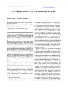
Fig. 2. Illustration of the image model for the case of two tissue types. (a) First, a label image L is drawn according to some statistical model (in this example, an MRF model was used; cf., further). (b) An intensity image Y is obtained by adding tissue-specific normally distributed noise. (c) Finally, Y is downsampled, resulting in an image Y~ that contains partial voluming. The underlying tissue fraction t = 1 t in each voxel i of Y~ is shown in (d), the histogram of Y along with its underlying model in (e), and the histogram of Y~ with its model in (f).
0
the numerical complexity, we only consider models that allow maximum two different tissue types in a voxel at the same time. To a first approximation, this assumption seems reasonable in MR images of the brain, and is shared by most of the methods described in the literature [16]–[22]. 1) Model A: No Spatial Correlation: Consider a spatial model defined on the observed voxels rather than on the underlying subvoxels, whereby the mixing proportions of tissues
in a voxel has a prior probability that is independent of the actual spatial position of the voxel in the image if if otherwise denotes a unity vector whose th element is unity, where all other elements being zero. In other words, the prior prob-
108
IEEE TRANSACTIONS ON MEDICAL IMAGING, VOL. 22, NO. 1, JANUARY 2003
ability to have a voxel that is entirely tissue type is , and for between every mixing fraction this is . Voxels with more than two classes and two tissue types at the same time are not allowed. The expectation step of the EM algorithm involves evaluating the probability of every possible mixing type in every voxel with Bayes’ rule
(2)
The subsequent maximization step involves finding the pa. Because rameters that maximize , the expectation function can be written as
Maximization of the B)
-term yields (see Appendix
(3)
To find the update of the parameters which yields have to maximize
, we
(5) To summarize, the EM algorithm iteratively calculates a statistical PV classification of the voxels based on the model parameters of the previous iteration [see (2)], and updates the parameters accordingly [see (3)–(5)]. The meaning of the equations becomes more intuitive in the special case where subvoxel underlying each voxel , i.e., there is only , there is no downsampling. In that case, meaning that each voxel belongs entirely to one single tissue type without PV effect. This reduces (3) and (4) to the equations shown at the bottom of the page, which are the well-known EM equations for standard Gaussian mixture models without PV model [2]. 2) Model B: No Spatial Correlation and Uniform Prior: In PV segmentation, it is common practice to assume that if two tissues mix in a voxel, all mixing proportions are equally alike [14], [17], [18]–[20], [22]. This can be imposed by explicitly constraining
in model A. Equations (2)–(4) for the classification and the subsequent calculation of the intensity parameters remain valid, but is now the update of the spatial parameters given by
and (4), shown at the bottom of the page, with
(4)
and
VAN LEEMPUT et al.: UNIFYING FRAMEWORK FOR PV SEGMENTATION OF BRAIN MR IMAGES
3) Model C: Markov Random Field: Finally, we investigate a MRF model [23] for the label image , defined as
109
Once samples are drawn, the maximization step of the EM algorithm proceeds as follows. A classification is obtained by summing the probabilities of all the subvoxel configurations with the same relative amounts of tissues , where (8)
with (6) evaluates to the unity value if the voxels Here, and belong to a different tissue type, and to zero otherwise; indicates that the summation is taken the notation that are nearest neighbors in over all couples of voxels the image grid and that include voxel . The spatial model paconsist of a that, when positive, rameters favors clusters of the same tissue , and of tissue-specific prior that regulate how much of tissue is globally present costs tissue types, this in the label image . In the case of model is the well-known Ising model [24]. Unfortunately, the expectation step of the EM algorithm poses practical problems with this model because the voxel labels are not independent. We, therefore, resort to the so-called Monte Carlo expectation-maximization algorithm [25] to by drawing approximate the expectation over the labels samples from the distribution by Monte Carlo simulation. are drawn using a Metropolis sampler The samples [26]. Suppose that the subvoxel label configurations of all the , are known. Then the voxels except voxel , denoted as in voxel prior probability for subvoxel label configuration is given by
the indicator function (valued 1 if , and 0 otherwith wise). From this classification, (3) and (4) are used to update the . The spatial parameters are updated intensity parameters that because of the Monte Carlo by maximizing simulation is approximated by
(9) [see Because the denominator in the expression for (6)] is impossible to calculate in practice, we call upon the so-called pseudolikelihood approximation [27] which gives finally
Because of (7), this approximation of is an from analytical function of the parameters which the first- and second-order derivatives can easily be calwith Newton’s culated. We, therefore, maximize method, i.e., by iteratively approximating the objective function locally by a quadratic model and calculating the maximum of that model. IV. EXPERIMENTS
(7) and so the posterior is given by
To generate a sample starting from , the sampler visits each voxel , proposes randomly a new label configuration and replaces the old configuration with the new one with probability
Starting from an initial label image, this scheme generates after a number samples from the distribution of so-called “warm up”-sweeps that are needed to bring the sampler in its stationary regime [26].
We have implemented the method in 2-D for each of the three different spatial models described in Section III, and applied it to analyze simulated data sets as well as 2-D slices of real MR data of the head. In each case, the iterative EM process was , and stopped when the started from an initial parameter set maximization step stops improving the parameters significantly (see [28] for more details on the stop criterion). For model C, the expectation step was approximated by drawing Monte Carlo samples for simulated data, and samples for real data. In the first iteration, the label image was randomly initialized and 100 “warm-up” Monte Carlo sweeps were performed before the samples were used. During the following iterations, we simply took the last sample from the previous iteration as initialization and used the generated samples immediately without “warm-up” phase. To give an idea of the computation time, the segmentation of a 2-D slice of a brain MR image took a couple of minutes when spatial model B was used, whereas the extensive Monte Carlo sampling of model C slowed the process down to 20 min (Matlab code [29] on a PC running Linux with a 1.70-GHz Pentium IV processor and 512-MB RAM). While this last time figure may seem prohibitively slow when full three-dimensional (3-D) images need to be analyzed, in reality the model
110
IEEE TRANSACTIONS ON MEDICAL IMAGING, VOL. 22, NO. 1, JANUARY 2003
(a)
(b)
(c)
(d)
(e)
(f)
(g)
(h)
(i)
(j)
(k)
(l)
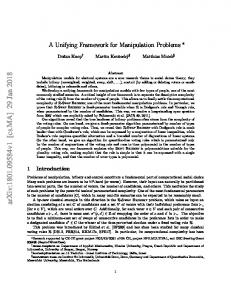
Fig. 3. PV segmentation of synthetic multi-spectral data in which the tissue types show considerable intensity overlap. The first six panels depict the synthetic data. The first channel and second channel of the 2-channel data Y~ is shown in (a) and (b), respectively. The scatterplot of this data is shown in (c), together with a semi-transparent 3-D envelope of the overall histogram model. Also shown are ellipses indicating a Mahalanobis distance of 2.5 in the underlying normal distributions corresponding to the two pure tissue types. The true underlying fraction of tissue 2 in each voxel in Y~ is depicted in (d), whereas the original label image L used to generate Y~ is shown in (e). Finally, the parameters used for initializing the EM algorithm are indicated on the scatterplot in (f). The last six panels show the result of the EM parameter estimation process for each of the three spatial models. The estimated parameters after model fitting and the expected fraction of tissue 2 are shown in (g) and (h), (i) and (j), and (k) and (l) for spatial model A, model B, and model C, respectively. (g), (i), and (k) Need to be compared with (c), and (h), (j), and (l) should be related to (d). See text for an interpretation.
parameter estimation for a 3-D image need not be more time consuming than for a 2-D slice. Indeed, the stationarity of model C implies that less samples are needed to estimate the model parameters accurately when more voxels are available in the image. Also, in our current implementation we generate samples at each a whole new set of . Considerable speed-ups can be expected by iteration using the recently proposed Stochastic Approximation EM algorithm [30] instead, in which simulated data from previous iterations are re-used, gradually discounted with a certain forgetting factor. Further speed-ups can be obtained by reducing the number of samples in the first iterations where the gross parameter adjustments are performed, but such optimization issues fall outside the scope of this text.
A. Experiments on Simulated Data In order to study the various model assumptions and their impact on the behavior of the EM parameter estimation process, we applied our algorithm on a number of synthetic images, using each of the three spatial models described in Section III. To obtain synthetic images in which the tissue types are spatially clustered, we started by drawing a sample from our MRF model C by starting from a random initialization and using 3000 sweeps of the Metropolis algorithm. From this sample we subsequently generated tissue-specific intensity and noise, resulting in , and after downsampling, we finally obtained . In this fashion, we generated synthetic data according to several sets of model parameters . Each data set represents a more or less realistic situation encountered in real-world PV segmentation of brain
VAN LEEMPUT et al.: UNIFYING FRAMEWORK FOR PV SEGMENTATION OF BRAIN MR IMAGES
TABLE I ERRORS IN VOLUME ESTIMATION ON SIMULATED MULTISPECTRAL PARTIAL VOLUME DATA WITH VARYING INTENSITY OVERLAP BETWEEN THE TISSUES FOR THREE DIFFERENT SPATIAL MODELS. HIGHER VALUES OF THE PARAMETER r CORRESPOND TO MORE SEVERE INTENSITY OVERLAP
MR images, including multi-spectral data, data that contains far more of one tissue than of another, and data in which one tissue type has an intensity that is indiscernible from a mixture of two other tissues. For each data set, the EM algorithm was used to try to find back the original model parameters underlying . This was done for each of the three different spatial models, starting from were initialized to the same initialization. The mean values the ground-truth mean values perturbed with zero-mean normally distributed noise with covariance matrix equal to the average of the ground-truth covariance matrices. The covariance were all initialized as the average covariance mamatrices trix multiplied by a factor of five. The spatial parameters were initially set to values that make the prior probability for all pure were and mixing tissues equally alike. For model A, the initialized uniformly for all mixing fractions . Since it is hard to interpret directly any differences between the true model parameters used to synthesize the data and the parameters estimated by the EM algorithm, we evaluated the correctness of the parameter estimations by comparing the automatically estimated volume of every tissue type in the entire image to the known ground-truth volume. Let denote the true the volume of a label total volume of tissue , and image estimated from . Since our algorithm does not produce a single label image , we compare the expected estimated volume with its true value
where denotes the model parameters estimated by the algorithm.
111
TABLE II ERRORS IN VOLUME ESTIMATION ON SIMULATED DATA WITH VARYING RELATIVE AMOUNTS OF PURE TISSUES. HIGHER VALUES OF THE PARAMETER a CORRESPOND TO SMALLER AMOUNTS OF TISSUE TYPE 1
B. Experiments on Real MR Data We also tested our algorithm on 2-D slices taken from real MR images of the brain. Our current implementation of the MRF of model C is only 2-D, i.e., the subvoxels are only subvoxels within the plane. This implies that borders are assumed to be orthogonal to the image slice and, therefore, we have only processed slices taken from the central part of the brain, where this assumption is more or less valid. In a preprocessing step, the images were automatically corrected for MR inhomogeneities and segmented into white matter, gray matter, CSF, and nonbrain tissue without taking the PV effect into account using the method described in [7]1 The resulting segmentations were used to automatically define the intracranial volume, and the PV fraction of white matter, gray matter, and CSF in each voxel of a selected slice within that volume was subsequently estimated subvoxels per voxel. with our new algorithm, using and were calculated from the segInitial parameters mentations obtained with the non-PV segmentation method, and the spatial model parameters were initialized in the same way as for the simulated data of Section IV-A. V. RESULTS A. Results on Simulated Data 1) Varying Intensity Overlap Between Tissues: In a first experiment, we simulated two-channel data with unequal covariance matrices whose size was varied in order to obtain a varying intensity overlap between the tissues. We used two classes and a 300 300 image grid that we downsampled by a factor of three in each dimension so that we finally ended up with a 100
1Software
publicly available at http://bilbo.esat.kuleuven.ac.be.
112
IEEE TRANSACTIONS ON MEDICAL IMAGING, VOL. 22, NO. 1, JANUARY 2003
(a)
(b)
(c)
(d)
(e)
(f)
Fig. 4. Model parameter estimation on synthetic data with considerable more amounts of one tissue type than of another. (a) Simulated data Y~ ; (b) histogram of with the underlying model superimposed; (c) initialization for the model estimation; (d) histogram fit after parameter estimation for model A, (e) model B, and (f) model C.
Y~
100 image with subvoxels per voxel. The model parameters used for the simulation were
with . Fig. 3 shows the simulated data for the biggest intensity ) along with the initialization and the results overlap ( for the three spatial models. In the scatter plots, we have indicated the shape of the normal distributions corresponding to pure tissue voxels by drawing the ellipse corresponding to a Mahalanobis distance of 2.5; note the considerable overlap in intensity between the tissues. According to Fig. 3(g), (i), and (k), all three methods seem to have found the correct model parameters. This is confirmed by Table I, showing small errors in total volume estimation for all models. Nevertheless, the expected fraction of tissue 2 in each voxel , depicted in Fig. 3(h), (j), and (l) for model A, B, and C, respectively, clearly indicates that the MRF of model C is better suited for estimating the relative amount of each tissue type in individual voxels. This should not come as a surprise, as the first two models classify each voxel independently based on local intensity information alone, whereas model C encourages exactly that type of spatial clustering that was used to synthesize the data. Since the overall model parameters were correctly estimated for all models, however, the classification errors in individual voxels of model A and B do not propagate into the total volume estimates of Table I because the errors cancel out when averaged over all voxels in the image.
2) Varying Relative Amounts of Pure Tissues: In a second experiment, we varied the relative amounts of tissues present in the underlying label image by assigning different prior costs to the classes. Again, two classes were used, the original image grid was 300 300, and we downsampled three times . The simulation parameters in each dimension so that were
Table II shows the volume estimation errors for all models and for every degree of asymmetry between tissue volumes. Model C always provides accurate volume estimations, in contrast to the other models that show large volume errors for the most asymmetric cases. This indicates that the parameters were not correctly estimated by models A and B. Fig. 4 clarifies these quantitative results for the case . While the global histogram fit is good for model A [Fig. 4(d)], the underlying model has been incorrectly estimated. The model has set the weights of the pure tissue voxels to zero, thereby not classifying any voxel in the image as of pure tissue. Since there is no restriction on the weights each mixing fraction , the method has simply adjusted these to get a good histogram fit. With model B, shown in Fig. 4(e), all the mixing fractions corresponding to nonpure tissues are , resulting in forced to have the same weight, i.e., the typical flat shape of the total intensity model for PV voxels that is commonly used in the literature [14], [17], [18]–[20], [22]. However, the true mixing fractions in this example are not equal at all and, therefore, model B is condemned to fail. Finally, Fig. 4(f) shows that only model C has succeeded in retrieving the correct model parameters.
VAN LEEMPUT et al.: UNIFYING FRAMEWORK FOR PV SEGMENTATION OF BRAIN MR IMAGES
TABLE III ERRORS IN VOLUME ESTIMATION ON SIMULATED DATA WITH VARYING AMOUNT OF PARTIAL VOLUME VOXELS. LOWER VALUES OF THE PARAMETER CORRESPOND TO LOWER AMOUNTS OF VOXELS CONTAINING PURE TISSUE TYPES
113
to be entirely based on the histogram. However, for this type of “difficult” data with considerable amounts of partial voluming, the histogram alone does not seem to provide enough information for robustly estimating the underlying model parameters. B. Results on Real MR Data
3) Varying Partial Voluming: We also simulated data for varying amounts of partial voluming, by varying the MRF parameter . We used three classes and an original image grid of 200 200 that was downsampled twice in each dimension subvoxels per so that is a 100 100 image with voxel. The simulation parameters were in this case
For the largest value of , 35% of the voxels were PV voxels, and for the smallest value this was 63%. Because the intensity of voxels mixing the tissues with the lowest and highest intensity is similar to the intensity of pure voxels of the tissue type with intermediate intensity, model A is severely underconstrained in this case and was, therefore, not considered. Table III summarizes the results for model B and model C. As in Section V-A2, the MRF seems indispensable to obtain accurate parameter estimates. Fig. 5 shows the graphical results for the case with the smallest amount of PV voxels ( ). Clearly, the mixing fractions between tissue 1 and tissue 3 do not all have the same weight, which partly explains why model C consistently performed better than model B in the results of Table III. However, the problem lies deeper than that. Fig. 5(d)–(f) depicts the initialization, the fitted model B, and the fitted model C, respectively. While the global histogram fit is equally good for both models, the underlying parameter estimates are only correct for model C. To illustrate this problem further, we repeated the same experiment but with another random initialization, the results of which are shown in Fig. 5(g)–(i). Although the initialization was very similar to that of Fig. 5(d), the parameters estimated for model B are now completely different. In contrast to model C, model B assumes statistical independence of the tissue proportions between the voxels, which causes its parameter estimation
Fig. 6(a) shows an axial slice of a high-resolution 1 mm isotropic T1-weighted image of the head (Siemens, 3-D MP-RAGE, TR 9.7 ms and TE 4 ms). Its histogram with the model parameter initialization overlaid is shown in Fig. 6(b). As with the simulated data set of Fig. 5, model A cannot be robustly applied because different tissue mixings map to the same intensities and was, therefore, not considered. For method B, the fitted model is shown in Fig. 6(c), and the estimated fractions of white matter, gray matter, and CSF are depicted in Fig. 6(d)–(f), respectively. At first sight, the results seem satisfactory, although the separation between white matter and gray matter is noisy. Fig. 6(g)–(i) shows for each voxel the probability that it is considered as partial voluming between white matter-gray matter, white matter-CSF, and gray matter-CSF, respectively. Except for a ridge around the ventricles, the voxels that are classified as partial voluming between white matter and CSF lie far away from white matter. This is clearly not correct. Fig. 7 shows the result on the same data set when model C was used. Because now also spatial information was used to estimate the model parameters, the histogram fit is not as tight as with model B. However, the MRF has reduced the noise in the segmentations considerably, and the voxels mixing two tissues are now lying on the border between the constituent tissues, which is clearly a much better result than the one obtained with method B. On the other hand, notice from Fig. 7(e) that the deep gray matter structures—in reality a mixture of white and gray matter—have been exclusively classified as gray matter, with sharp borders. This, and other limitations that are intrinsic to our MRF model, hampers its direct use in many practical situations as will be discussed further in Section VI-C. VI. DISCUSSION A. Related Work In the existing literature about PV segmentation of MR brain images, two approaches have been followed that mainly differ in the prior assumptions about the spatial distribution of the tissue types in the images. The first approach, initiated by Santago and Gage [18], [19], discards all spatial dependence of the tissue fractions between the voxels, and explicitly assumes a uniform prior probability for all nonpure tissues. Under these assumptions, Santago and Gage derived the intensity distribution for partial voluming between two normally distributed tissue types, and estimated the parameters of the resulting model by minimizing the distance between the histogram and the model. While Santago and Gage only addressed the problem of estimating the total volume of each tissue in an entire image, their work was extended by other authors to estimate the amount of every tissue in each individual voxel. Replacing Santago and Gage’s carefully derived PV model by a new, independent distribution and fitting this
114
IEEE TRANSACTIONS ON MEDICAL IMAGING, VOL. 22, NO. 1, JANUARY 2003
(a)
(b)
(c)
(d)
(e)
(f)
(g)
(h)
(i)
Fig. 5. Results for simulated data with three tissue classes: (a) label image L ; (b) resulting partial volumed image Y~ ; and (c) histogram of Y~ with the ground-truth model superimposed. (d)–(f) Model initialization, the histogram fit for model B, and the histogram fit for model C, respectively. (g)–(i) Same as (d)–(f), but starting from a different initialization. Notice that the parameter estimations with model B are incorrect and different for different initializations.
simplified model to the histogram, Laidlaw et al. [20] used the intensity of a voxel and that of its neighbors to determine the mixing proportions in a voxel. However, because of their simplification of the PV distribution, they had to introduce an heuristic division rule for voxels classified to this distribution that is not further justified. In a similar vein, Ruan et al. [17] simply replaced the PV distributions with independent normal distributions. After fitting the model to the histogram, each voxel was uniquely assigned to one single pure tissue type using a MRF prior and a feature that is highly T1-specific, thereby loosing all notion of partial voluming. Shattuck et al. [21] used Santago and Gage’s PV model to classify T1-weighted brain MR images based on a sequence of low-level operations. The second approach is based on the notion that the mixing proportions change “smoothly” over the voxels in real-world images, where “smoothly” is imposed by a MRF model [31], [32], [16]. Assuming that the noise in the images is tissue-independent and that the noise characteristics and the mean intensities of the pure tissue types are known a priori, Choi et al. [31] searched for the maximum a posteriori (MAP) PV segmentation by iteratively looking for the best classification of every voxel based on the intermediate classification of its neighbors. They also described two heuristic ways to update the mean in-
tensities of the pure tissues, based on thresholds defining what is pure tissue and what not. Pham and Prince [16] proposed a single-channel method that is very similar, with a different MRF and with an updating rule for the mean intensities that relies on some heuristic prior. Finally, Nocera and Gee [32] used a gradient-descent search algorithm to find the MAP segmentation; they also allowed the mean intensities to vary spatially smoothly to compensate for MR inhomogeneities. B. A Unifying Framework The method proposed in this paper tackles the problem of PV segmentation of brain MR images from a different angle. In a model-based EM framework, widely used to classify brain MR images into pure tissue types, an additional downsampling step was introduced that accounts for partial voluming along the borders between tissues. The resulting segmentation algorithm is a natural extension of the usual EM approach, estimating the relative amounts of the various tissue types in each voxel rather than simply assigning each voxel to one single tissue. Remarkably, our EM approach provides a sound mathematical framework that encompasses the existing PV methods described in Section VI-A, avoiding all heuristic steps and algorithmic tuning. Indeed, our spatial model B describes exactly the
VAN LEEMPUT et al.: UNIFYING FRAMEWORK FOR PV SEGMENTATION OF BRAIN MR IMAGES
(a)
(b)
115
(c)
(d)
(e)
(f)
(g)
(h)
(i)
Fig. 6. PV segmentation of an axial slice of a high-resolution T1-weighted image when spatial model B was used: (a) data Y~ ; (b) histogram with the initialization superimposed; (c) histogram fit after model estimation; (d) expected fraction of white matter, (e) gray matter, and (f) CSF; (g) estimated probability for partial voluming between white matter-gray matter, (h) white matter-CSF, and (i) gray matter-CSF.
statistical independence of the tissue fractions between voxels and the uniform prior probability for nonpure tissue types assumed in the work of Santago and Gage [18], [19], Laidlaw et al. [20] and Ruan et al. [17]. When model B is used, our method offers an alternative parameter estimation technique for these methods, optimizing the likelihood of the model instead of its distance to the histogram. However, our EM approach estimates the model parameters and the tissue classification at the same time, rather than in two separate processing steps. As will be discussed in Section VI-C, this offers the vital advantage that spatial information can keep the model parameter estimation well-determined in cases where the histogram alone does not provide sufficient information to uniquely define the model parameters. With spatial model C, i.e., the MRF model, our algorithm encompasses the PV segmentation methods of Choi et al. [31], Pham and Prince [16] and Nocera and Gee [32]. These methods iteratively assign one single mixing type to each voxel based on a MRF prior, and update the mean intensity of every pure tissue
type accordingly. Our approach extends these techniques by additionally tackling the difficult problem of estimating tissue-dependent intensity covariances as well. Also, there is a conceptual difference between the tissue fractions, that are random variables in the model, and the mean intensities, that are model parameters. It is well known that optimizing both simultaneously as in [31], [16], [32] may introduce severe biases in the model parameter estimation [33]. Indeed, imagine that each voxel is uniquely assigned to the normal distribution with the highest probability for its intensity in Fig. 2(f). Because of the large overlap between the normal distributions, this would produce a set of rectangularly truncated regions of the histogram to which the normal distributions are subsequently fitted, introducing severe errors in the parameter estimation. In our approach, on the contrary, all possible mixing types are considered and conto the parameter estimation. tribute with a fraction This divides the histogram into overlapping normal distributions ensuring that no bias is incurred on the subsequent model parameter estimation [33].
116
IEEE TRANSACTIONS ON MEDICAL IMAGING, VOL. 22, NO. 1, JANUARY 2003
(a)
(b)
(c)
(d)
(e)
(f)
(g)
(h)
(i)
Fig. 7. PV segmentation of the same MR slice as in Fig. 6, but when model C was used as a spatial prior instead. Subfigures (g)–(i) need to be compared to the corresponding subfigures in Fig. 6; notice how much better the voxels mixing two tissues are now lying on the border between the constituent tissues.
C. Spatial Models As we have shown, our approach presents a global framework for PV segmentation in which various statistical spatial models can be easily integrated. The selection of an appropriate spatial model, however, turns out to be a difficult issue. The most trivial choice is our model A, which simply assumes statistical independence of the tissue proportions between the voxels, without further premises concerning the overall amount of specific mixing types. While this yields a very flexible model that can describe virtually any kind of image, the lack of spatial dependency between the voxels causes the parameter estimation to be entirely based on the histogram. Because of the complexity of the model, this leads to severely underconstrained estimation problems, even in the simplest case where merely two tissue types mix as in Fig. 4. A popular way to decrease the abundant number of degrees of freedom in the model, is to assume that all nonpure mixing combinations between two tissue types are equally alike [14], [17]–[20], [22]. This is our model B. However, such a
simple model is in contradiction with experimental evidence. Röll et al. [34] showed that not all mixing proportions occur equally frequently when spheres are sampled on a 3-D image grid. Figs. 2(f) and 4(b) demonstrate that the same is true for realizations of the Ising MRF model. Besides, the assumption of a uniform prior for nonpure tissue types does not tackle the underconstrained nature of the parameter estimation adequately in cases with considerable amounts of partial voluming. In the simulated data of Fig. 5, slight modifications in the initialization resulted in very different estimated parameter sets with model B that nevertheless all provided a close fit to the histogram. Such situations also occur in real MR images of the brain with 1 1 mm data a lower resolution than the isotropic 1 shown in Figs. 6 and 7. Fig. 8 shows the intracranial volume of a T2-weighted image of the head (TR 3800 ms and TE 90 ms; 20 axial slices; pixel size: 1.18 1.18 mm ; slice thickness: 3 mm; and interslice gap: 3 mm), along with just a few of the possible explanatory parameter sets overlaid on its histogram when model B is used. Because high amounts of PV voxels mask away the peaks corresponding to pure gray matter and
VAN LEEMPUT et al.: UNIFYING FRAMEWORK FOR PV SEGMENTATION OF BRAIN MR IMAGES
(a)
117
(b)
(c)
(d)
Fig. 8. In lower resolution MR images of the brain, it is often impossible to estimate the model parameters from the histogram alone. This example shows the intracranial volume of a T2-weighted MR scan with a slice thickness of 3 mm. (a) Shows an axial slice, whereas (b)–(d) depict the histogram with some of the possible explanatory parameter sets overlaid when model B is used.
CSF, the histogram alone does not seem to provide enough information to uniquely define the model parameters. Clearly, a more intelligent way to make the parameter estimation well-determined is needed. What discerns the desired parameter set from other ones that model the histogram equally well, is that it additionally provides a meaningful classification. In Section V, we showed on simulated data that using a spatial model that favors the desired type of classifications enables robust parameter estimation even in very difficult cases. In order to come to general, robust PV segmentation of brain MRI, the aim is, therefore, to construct spatial models that somehow describe the spatial distribution of tissues in the human brain. Choi et al. [31] and Nocera and Gee [32] proposed a MRF model that imposes similar brain tissue fractions over neighboring voxels. However, their model is too simple as the optimal solution is given by values of that mix all tissues in equal amounts everywhere in the image, and extreme values for . Indeed, some of the normal distributions that model PV voxels are sufficient to provide a close histogram fit, very similar to the situation shown in Fig. 4(d), and the MRF prior erroneously encourages this solution. Pham and Prince [16] used a MRF model that besides imposing similar tissue types in neighboring voxels, explicitly favors regions of pure tissue. However, they had to introduce heuristics to prevent the means from taking extreme values, indicating that the MRF problem might not have been totally solved.
In contrast, our model C defines an Ising MRF model on subvoxels rather than directly on the voxels, thereby naturally imposing homogeneous regions of pure tissues bordered by PV voxels. The advantage of this approach on real MR images of the brain is clearly visible from Fig. 7. Unfortunately, however, the model in its current form seems too simplistic to be generally applicable. Since it only allows PV voxels at the interface between two tissues, it is not able to describe such structures as the deep gray matter where white and gray matter truly mix without interface (cf., Fig. 7). Also, the Ising model tempts to minimize the boundary length between tissues [35], which discourages classifications from accurately following the highly convoluted shape of the complex human cortex. This effect is amplified by the presence of large uniform regions of single tissue types in brain images, which results in very high estimates for the MRF class transition costs and, thus, a strong favor for smooth boundaries. In contrast to high-resolution data, the intensity information of lower resolution images with histograms similar to Fig. 8(b) does not provide a suitable counterweight for such a strong prior, resulting in seriously oversmoothed segmentation results when model C is used. It is, however, exactly in those difficult cases that the MRF has to play its crucial role of providing the adequate spatial information. While we have provided in this paper a sound mathematical framework for PV segmentation of MR images of the brain, the construction of a suitable spatial model to be used within this
118
IEEE TRANSACTIONS ON MEDICAL IMAGING, VOL. 22, NO. 1, JANUARY 2003
framework remains a challenging task for future research. A nonstationary Ising model, with different parameters in uniform regions of pure tissue than at places where tissues mix, might be a promising starting point. Such a MRF may be guided by atlas information, as suggested in [16]. We believe that research to improved spatial models is the key to providing the indispensable prior information that is necessary for general robust PV segmentation of MR images of the brain.
with
which explains (1). APPENDIX B
APPENDIX A Here, we derive the expression for It can easily be shown that
used in (1).
The EM update for the intensity parameters by maximization of
are given
(10) where and
For , this yields (11) as shown at the bottom of the page, denotes the indicator function. Using the same notawhere tion as in Appendix A, we have
Assume without loss of generality that the indexes of the subvoxels underlying voxel are given by . Then
where (10) was used and the property that . times, we finally get Applying the same technique
(11)
VAN LEEMPUT et al.: UNIFYING FRAMEWORK FOR PV SEGMENTATION OF BRAIN MR IMAGES
(12) To come to the third-last equation, the same technique was applied as the one used in Appendix A, and the second-last equation is obtained by application of (10). Filling (12) in into (11) finally yields (3). is analogous. The derivation of (4) for REFERENCES [1] A. P. Dempster, N. M. Laird, and D. B. Rubin, “Maximum likelihood from incomplete data via the EM algorithm,” J. Roy. Statist. Soc., vol. 39, pp. 1–38, 1977. [2] Z. Liang, J. R. MacFall, and D. P. Harrington, “Parameter estimation and tissue segmentation from multispectral MR images,” IEEE Trans. Med. Imag., vol. 13, pp. 441–449, Sept. 1994. [3] P. Schroeter, J.-M. Vesin, T. Langenberger, and R. Meuli, “Robust parameter estimation of intensity distributions for brain magnetic resonance images,” IEEE Trans. Med. Imag., vol. 17, pp. 172–186, Apr. 1998. [4] D. L. Wilson and J. A. Noble, “An adaptive segmentation algorithm for time-of-flight MRA data,” IEEE Trans. Med. Imag., vol. 18, pp. 938–945, Oct. 1999. [5] W. M. Wells, III, W. E. L. Grimson, R. Kikinis, and F. A. Jolesz, “Adaptive segmentation of MRI data,” IEEE Trans. Med. Imag., vol. 15, pp. 429–442, Aug. 1996. [6] R. Guillemaud and M. Brady, “Estimating the bias field of MR images,” IEEE Trans. Med. Imag., vol. 16, pp. 238–251, June 1997. [7] K. Van Leemput, F. Maes, D. Vandermeulen, and P. Suetens, “Automated model-based bias field correction of MR images of the brain,” IEEE Trans. Med. Imag., vol. 18, pp. 885–896, Oct. 1999. [8] K. Held, E. R. Kops, B. J. Krause, W. M. Wells, III, R. Kikinis, and H. W. Müller-Gärtner, “Markov random field segmentation of brain MR images,” IEEE Trans. Med. Imag., vol. 16, pp. 878–886, Dec. 1997. [9] T. Kapur, W. E. L. Grimson, R. Kikinis, and W. M. Wells, “Enhanced spatial priors for segmentation of magnetic resonance imaging,” in Lecture Notes in Computer Science. Berlin, Germeny: Springer-Verlag, 1998, vol. 1496, Proceedings of Medical Image Computing and Computer-Assisted Intervention—MICCAI’98, pp. 457–468. [10] K. Van Leemput, F. Maes, D. Vandermeulen, and P. Suetens, “Automated model-based tissue classification of MR images of the brain,” IEEE Trans. Med. Imag., vol. 18, pp. 897–908, Oct. 1999. [11] Y. Zhang, M. Brady, and S. Smith, “Segmentation of brain MR images through a hidden markov random field model and the Expectation Maximization algorithm,” IEEE Trans. Med. Imag., vol. 20, pp. 45–57, Jan. 2001. [12] K. Van Leemput, F. Maes, D. Vandermeulen, A. Colchester, and P. Suetens, “Automated segmentation of multiple sclerosis lesions by model outlier detection,” IEEE Trans. Med. Imag., vol. 20, pp. 677–688, Aug. 2001. [13] W. J. Niessen, K. L. Vincken, J. Weickert, B. M. ter Haar Romeny, and M. A. Viergever, “Multiscale segmentation of three-dimensional MR brain images,” Int. J. Comput. Vis., vol. 31, no. 2/3, pp. 185–202, 1999.
119
[14] Z. Wu, H.-W. Chung, and F. W. Wehrli, “A bayesian approach to subvoxel tissue classification in NMR microscopic images of trabecular bone,” MRM, vol. 31, pp. 302–308, 1994. [15] C. F. J. Wu, “On the convergence properties of the EM algorithm,” Ann. Statist., vol. 11, no. 1, pp. 95–103, 1983. [16] D. L. Pham and J. L. Prince, “Unsupervised partial volume estimation in single-channel image data,” in Proc. IEEE Workshop Mathematical Methods in Biomedical Image Analysis—MMBIA’00, 2000, pp. 170–177. [17] S. Ruan, C. Jaggi, J. Xue, J. Fadili, and D. Bloyet, “Brain tissue classification of magnetic resonance images using partial volume modeling,” IEEE Trans. Med. Imag., vol. 19, pp. 1179–1187, Dec. 2000. [18] P. Santago and H. D. Gage, “Quantification of MR brain images by mixture density and partial volume modeling,” IEEE Trans. Med. Imag., vol. 12, pp. 566–574, Sept. 1993. [19] P. Santago and H. D. Gage, “Statistical models of partial volume effect,” IEEE Trans. Image Processing, vol. 4, pp. 1531–1540, Nov. 1995. [20] D. H. Laidlaw, K. W. Fleischer, and A. H. Barr, “Partial-volume bayesian classification of material mixtures in MR volume data using voxel histograms,” IEEE Trans. Med. Imag., vol. 17, pp. 74–86, Feb. 1998. [21] D. W. Shattuck, S. R. Sandor-Leahy, K. A. Schaper, D. A. Rottenberg, and R. M. Leahy, “Magnetic resonance image tissue classification using a partial volume model,” NeuroImage, vol. 13, no. 5, pp. 856–876, 2001. [22] M. A. González Ballester, “Morphometric analysis of brain structures in MRI,” Ph.D. dissertation, Dept. Eng. Sci, Univ. Oxford, Oxford, U.K., 1999. [23] S. Z. Li, Markov Random Field Modeling in Computer Vision: Springer, Computer Science Workbench, 1995. [24] E. Ising, “Beitrag zur theorie des ferromagnetismus,” Zeitschrift für Physik, vol. 31, pp. 253–258, 1925. [25] G. C. G. Wei and M. Tanner, “A Monte Carlo implementation of the EM algorithm and the poor man’s data augmentation algorithm,” J. Amer. Statist. Assoc., vol. 85, pp. 699–704, 1990. [26] N. Metropolis, A. Rosenbluth, and A. Teller, “Equations of state calculations by fast computing machines,” J. Chem. Phys., vol. 21, pp. 1087–1092, 1953. [27] J. Besag, “Efficiency of pseudo-likelihood estimation for simple Gaussian fields,” Biometrika, vol. 64, pp. 616–618, 1977. [28] K. Van Leemput, F. Maes, D. Vandermeulen, and P. Suetens. (2001, Apr.) A statistical framework for partial volume segmentation. K. U. Leuven, Leuven, Belgium. [Online]. Available: http://bilbo.esat.kuleuven.ac.be, Tech. Rep. KUL/ESAT/PSI/0102 [29] “Matlab,” The MathWorks Inc., Natick, MA. [30] B. Delyon, M. Lavielle, and E. Moulines, “Convergence of a stochastic approximation version of the EM algorithm,” Ann. Statist., vol. 27, no. 1, pp. 94–128, 1999. [31] H. S. Choi, D. R. Haynor, and Y. Kim, “Partial volume tissue classification of multichannel magnetic resonance images—A mixel model,” IEEE Trans. Med. Imag., vol. 10, pp. 395–407, Sept. 1991. [32] L. Nocera and J. C. Gee, “Robust partial volume tissue classification of cerebral MRI scans,” in Proceedings of SPIE Medical Imaging 1997: Image Processing, K. M. Hanson, Ed. Bellingham, WA: SPIE, 1997, vol. 3034 of SPIE Proceedings, pp. 312–322. [33] D. M. Titterington, “Comments on ‘application of the conditional population-mixture model to image segmentation’,” IEEE Trans. Pattern Anal. Machine Intell., vol. MI-6, pp. 656–658, Sept. 1984. [34] S. A. Röll, A. C. F. Colchester, P. E. Summers, and L. D. Griffin, “Intensity-based object extraction from 3D medical images including a correction for partial volume errors,” in Proc. BMVC‘94, E. Hancock, Ed., 1994, pp. 205–214. [35] R. D. Morris, X. Descombes, and J. Zerubia, “The Ising/Potts model is not well suited to segmentation tasks,” presented at the IEEE Digital Signal Processing Workshop, Loen, Norway, Sept. 1996.