... would like to thank everyone involved with Drexel's Vanguard Program, Diversity and .... 3. Framework of A Unit Cell based Multi-scale Modeling Approach for ...
A Unit Cell Based Multi-scale Modeling and Design Approach for Tissue Engineered Scaffolds A Thesis Submitted to the Faculty of Drexel University by Connie Gomez in partial fulfillment of the requirements for the degree of Ph.D. in Mechanical Engineering August 2007
c Copyright August 2007
Connie Gomez. This work is licensed under the terms of the Creative Commons AttributionShareAlike license. The license is available at http://creativecommons.org/ licenses/by-sa/2.0/.
ii
1. ACKNOWLEDGEMENTS
I would like to offer my sincerest and deepest gratitude to both my advisors, Dr. Wei Sun and Dr. Ali Shokoufandeh. Each one has offered me their guidance and encouragement throughout my graduate studies as well as a high professional standard to hold myself to now and as I pursue a career in academia. I would like to thank my committee members, Dr. Jack Zhou, Dr. Christopher Li, Dr. MinJun Kim, for their participation, time and recommendations. I would like to make special acknowledgments to all my lab members Zhibin, Ganesh, Binil, Saif, Andrew, Milind, Lauren, Kalyani, Bobby, Eda, Jie, Jae, Peter, Jennifer, Pat, Luly, and XY. Each of you brought something special to my research and my life. I will miss all of you. Additionally, I would like to thank the members of the Applied Algorithms Lab. Fatih, Trip, Jeff, John, and Craig whose collaborations and discussions were vital to me as I encountered more and more computer science. Last but not least, I would like to thank everyone involved with Drexel’s Vanguard Program, Diversity and Retention, ACT101, and SUCCESS. I would like to thank you all for maintaining my spirits and providing me with opportunities to grow. I would especially like to thank Antoinette Torres, who brought me to Drexel in the first place.
iii
Dedications Quiero dedicar este trabajo a mis padres, quienes me han apoyado sin siempre entender el camino que he decidido tomar en mi vida.
iv
Table of Contents 1. ACKNOWLEDGEMENTS . . . . . . . . . . . . . . . . . . . . . . . . . . . . . . . . . . . . . . . . . . . . . . . . . . . . . . . . . . . . . . . . . . . . . . . . . . . . . . .
ii
List of Figures . . . . . . . . . . . . . . . . . . . . . . . . . . . . . . . . . . . . . . . . . . . . . . . . . . . . . . . . . . . . . . . . . . . . . . . . . . . . . . . . . . . . . . . . . . . . . . . . . viii Abstract . . . . . . . . . . . . . . . . . . . . . . . . . . . . . . . . . . . . . . . . . . . . . . . . . . . . . . . . . . . . . . . . . . . . . . . . . . . . . . . . . . . . . . . . . . . . . . . . . . . . . . . . xv 2. INTRODUCTION . . . . . . . . . . . . . . . . . . . . . . . . . . . . . . . . . . . . . . . . . . . . . . . . . . . . . . . . . . . . . . . . . . . . . . . . . . . . . . . . . . . . . . . . .
1
2.1
Tissue Engineering. . . . . . . . . . . . . . . . . . . . . . . . . . . . . . . . . . . . . . . . . . . . . . . . . . . . . . . . . . . . . . . . . . . . . . . . . . . . . . . . . . .
1
2.2
Computer Aided Tissue Engineering . . . . . . . . . . . . . . . . . . . . . . . . . . . . . . . . . . . . . . . . . . . . . . . . . . . . . . . . . . . . . . .
3
2.2.1
Computer Aided Tissue Modeling . . . . . . . . . . . . . . . . . . . . . . . . . . . . . . . . . . . . . . . . . . . . . . . . . . . . . . . . .
5
2.2.2
Computer Aided Tissue Informatics . . . . . . . . . . . . . . . . . . . . . . . . . . . . . . . . . . . . . . . . . . . . . . . . . . . . . . .
5
2.2.3
Computer Aided Tissue Manufacturing . . . . . . . . . . . . . . . . . . . . . . . . . . . . . . . . . . . . . . . . . . . . . . . . . . . .
5
Scaffold Based Tissue Engineering . . . . . . . . . . . . . . . . . . . . . . . . . . . . . . . . . . . . . . . . . . . . . . . . . . . . . . . . . . . . . . . . .
6
2.3.1
Challenges in Scaffold Guided Tissue Engineering . . . . . . . . . . . . . . . . . . . . . . . . . . . . . . . . . . . . . . .
7
Research Objectives and Thesis Contributions . . . . . . . . . . . . . . . . . . . . . . . . . . . . . . . . . . . . . . . . . . . . . . . . . . . . .
7
2.4.1
Multi-scale Modeling and Design using a Unit Cell Structure . . . . . . . . . . . . . . . . . . . . . . . . . . .
8
2.4.2
Establishing Connectivity Criteria and Unit Cell Characterization . . . . . . . . . . . . . . . . . . . . . .
8
2.4.3
Assembly Unit Cells into a Scaffold . . . . . . . . . . . . . . . . . . . . . . . . . . . . . . . . . . . . . . . . . . . . . . . . . . . . . . .
8
2.4.4
Topology based Unit Cell Design . . . . . . . . . . . . . . . . . . . . . . . . . . . . . . . . . . . . . . . . . . . . . . . . . . . . . . . . . .
8
Thesis Outline . . . . . . . . . . . . . . . . . . . . . . . . . . . . . . . . . . . . . . . . . . . . . . . . . . . . . . . . . . . . . . . . . . . . . . . . . . . . . . . . . . . . . . . .
9
2.3
2.4
2.5
3. Framework of A Unit Cell based Multi-scale Modeling Approach for Biomimetic Design . . . . . . . . . . . 12 3.1
Introduction . . . . . . . . . . . . . . . . . . . . . . . . . . . . . . . . . . . . . . . . . . . . . . . . . . . . . . . . . . . . . . . . . . . . . . . . . . . . . . . . . . . . . . . . . . 12
3.2
Multi-scale Characteristics of Bone Tissue . . . . . . . . . . . . . . . . . . . . . . . . . . . . . . . . . . . . . . . . . . . . . . . . . . . . . . . . . 13
3.3
3.2.1
Micro-Scale Characteristics of Bone . . . . . . . . . . . . . . . . . . . . . . . . . . . . . . . . . . . . . . . . . . . . . . . . . . . . . . . 13
3.2.2
Macro-Scale Characteristics of Bone . . . . . . . . . . . . . . . . . . . . . . . . . . . . . . . . . . . . . . . . . . . . . . . . . . . . . . 14
3.2.3
The Meso-scale. . . . . . . . . . . . . . . . . . . . . . . . . . . . . . . . . . . . . . . . . . . . . . . . . . . . . . . . . . . . . . . . . . . . . . . . . . . . . . 14
Unit Cell based Scaffolds . . . . . . . . . . . . . . . . . . . . . . . . . . . . . . . . . . . . . . . . . . . . . . . . . . . . . . . . . . . . . . . . . . . . . . . . . . . . 15 3.3.1
Unit Cell Design . . . . . . . . . . . . . . . . . . . . . . . . . . . . . . . . . . . . . . . . . . . . . . . . . . . . . . . . . . . . . . . . . . . . . . . . . . . . 16
3.3.2
Unit Cell Characterization . . . . . . . . . . . . . . . . . . . . . . . . . . . . . . . . . . . . . . . . . . . . . . . . . . . . . . . . . . . . . . . . . . 17
3.3.3
Unit Cell Assembly . . . . . . . . . . . . . . . . . . . . . . . . . . . . . . . . . . . . . . . . . . . . . . . . . . . . . . . . . . . . . . . . . . . . . . . . . 17
3.3.4
Fabrication of a Unit Cell based Scaffold . . . . . . . . . . . . . . . . . . . . . . . . . . . . . . . . . . . . . . . . . . . . . . . . . . 18
3.4
Case Study . . . . . . . . . . . . . . . . . . . . . . . . . . . . . . . . . . . . . . . . . . . . . . . . . . . . . . . . . . . . . . . . . . . . . . . . . . . . . . . . . . . . . . . . . . . 18
3.5
Conclusions . . . . . . . . . . . . . . . . . . . . . . . . . . . . . . . . . . . . . . . . . . . . . . . . . . . . . . . . . . . . . . . . . . . . . . . . . . . . . . . . . . . . . . . . . . 21
v
4. Unit Cell Informatics and Unit Cell Characterization . . . . . . . . . . . . . . . . . . . . . . . . . . . . . . . . . . . . . . . . . . . . . . . . . . . 22 4.1
Introduction . . . . . . . . . . . . . . . . . . . . . . . . . . . . . . . . . . . . . . . . . . . . . . . . . . . . . . . . . . . . . . . . . . . . . . . . . . . . . . . . . . . . . . . . . . 22
4.2
Defining Unit Cell Criteria . . . . . . . . . . . . . . . . . . . . . . . . . . . . . . . . . . . . . . . . . . . . . . . . . . . . . . . . . . . . . . . . . . . . . . . . . . 22 4.2.1
Unit Cell Design Considerations . . . . . . . . . . . . . . . . . . . . . . . . . . . . . . . . . . . . . . . . . . . . . . . . . . . . . . . . . . . 22
4.2.2
Fabrication Design Considerations . . . . . . . . . . . . . . . . . . . . . . . . . . . . . . . . . . . . . . . . . . . . . . . . . . . . . . . . . 25
4.2.3
Unit Cell Parameters . . . . . . . . . . . . . . . . . . . . . . . . . . . . . . . . . . . . . . . . . . . . . . . . . . . . . . . . . . . . . . . . . . . . . . . . 25
4.3
Geometrical Characterization . . . . . . . . . . . . . . . . . . . . . . . . . . . . . . . . . . . . . . . . . . . . . . . . . . . . . . . . . . . . . . . . . . . . . . . 26
4.4
Constitutive Characterization. . . . . . . . . . . . . . . . . . . . . . . . . . . . . . . . . . . . . . . . . . . . . . . . . . . . . . . . . . . . . . . . . . . . . . . . 28
4.5
Mechanical Characterization . . . . . . . . . . . . . . . . . . . . . . . . . . . . . . . . . . . . . . . . . . . . . . . . . . . . . . . . . . . . . . . . . . . . . . . . 28 4.5.1
Rule-of-Mixtures . . . . . . . . . . . . . . . . . . . . . . . . . . . . . . . . . . . . . . . . . . . . . . . . . . . . . . . . . . . . . . . . . . . . . . . . . . . . 29
4.5.2
Finite Element Analysis . . . . . . . . . . . . . . . . . . . . . . . . . . . . . . . . . . . . . . . . . . . . . . . . . . . . . . . . . . . . . . . . . . . . 29
4.5.3
Homogenization Theory . . . . . . . . . . . . . . . . . . . . . . . . . . . . . . . . . . . . . . . . . . . . . . . . . . . . . . . . . . . . . . . . . . . . 29
4.6
Transport Characterization . . . . . . . . . . . . . . . . . . . . . . . . . . . . . . . . . . . . . . . . . . . . . . . . . . . . . . . . . . . . . . . . . . . . . . . . . . 30
4.7
Conclusions . . . . . . . . . . . . . . . . . . . . . . . . . . . . . . . . . . . . . . . . . . . . . . . . . . . . . . . . . . . . . . . . . . . . . . . . . . . . . . . . . . . . . . . . . . 30
5. Connectivity and Unit Cell Assembly . . . . . . . . . . . . . . . . . . . . . . . . . . . . . . . . . . . . . . . . . . . . . . . . . . . . . . . . . . . . . . . . . . . . 35 5.1
Introduction . . . . . . . . . . . . . . . . . . . . . . . . . . . . . . . . . . . . . . . . . . . . . . . . . . . . . . . . . . . . . . . . . . . . . . . . . . . . . . . . . . . . . . . . . . 35
5.2
Unit Cell Selection . . . . . . . . . . . . . . . . . . . . . . . . . . . . . . . . . . . . . . . . . . . . . . . . . . . . . . . . . . . . . . . . . . . . . . . . . . . . . . . . . . . 35
5.3
5.4
5.5
5.2.1
Unit Cell Fitness . . . . . . . . . . . . . . . . . . . . . . . . . . . . . . . . . . . . . . . . . . . . . . . . . . . . . . . . . . . . . . . . . . . . . . . . . . . . 36
5.2.2
Unit Cell Candidate Selection . . . . . . . . . . . . . . . . . . . . . . . . . . . . . . . . . . . . . . . . . . . . . . . . . . . . . . . . . . . . . . 38
5.2.3
Unit Cell Alignment Algorithm . . . . . . . . . . . . . . . . . . . . . . . . . . . . . . . . . . . . . . . . . . . . . . . . . . . . . . . . . . . . 38
5.2.4
Ranking . . . . . . . . . . . . . . . . . . . . . . . . . . . . . . . . . . . . . . . . . . . . . . . . . . . . . . . . . . . . . . . . . . . . . . . . . . . . . . . . . . . . . . 41
5.2.5
Alignment algorithm . . . . . . . . . . . . . . . . . . . . . . . . . . . . . . . . . . . . . . . . . . . . . . . . . . . . . . . . . . . . . . . . . . . . . . . . 44
Determining Mechanical Properties Using the Rule-of-Mixtures . . . . . . . . . . . . . . . . . . . . . . . . . . . . . . . . . 45 5.3.1
Assumptions . . . . . . . . . . . . . . . . . . . . . . . . . . . . . . . . . . . . . . . . . . . . . . . . . . . . . . . . . . . . . . . . . . . . . . . . . . . . . . . . . 46
5.3.2
Rule of Mixtures . . . . . . . . . . . . . . . . . . . . . . . . . . . . . . . . . . . . . . . . . . . . . . . . . . . . . . . . . . . . . . . . . . . . . . . . . . . . 47
5.3.3
Stiffness Matrix Cij . . . . . . . . . . . . . . . . . . . . . . . . . . . . . . . . . . . . . . . . . . . . . . . . . . . . . . . . . . . . . . . . . . . . . . . . . 51
5.3.4
Transformation . . . . . . . . . . . . . . . . . . . . . . . . . . . . . . . . . . . . . . . . . . . . . . . . . . . . . . . . . . . . . . . . . . . . . . . . . . . . . . 53
Connectivity Criteria. . . . . . . . . . . . . . . . . . . . . . . . . . . . . . . . . . . . . . . . . . . . . . . . . . . . . . . . . . . . . . . . . . . . . . . . . . . . . . . . . 54 5.4.1
Criterion for Connectivity between 1D . . . . . . . . . . . . . . . . . . . . . . . . . . . . . . . . . . . . . . . . . . . . . . . . . . . . 55
5.4.2
Criterion for Connectivity between 2D . . . . . . . . . . . . . . . . . . . . . . . . . . . . . . . . . . . . . . . . . . . . . . . . . . . . 56
5.4.3
Example . . . . . . . . . . . . . . . . . . . . . . . . . . . . . . . . . . . . . . . . . . . . . . . . . . . . . . . . . . . . . . . . . . . . . . . . . . . . . . . . . . . . . 58
Skeleton Representation of Unit Cells . . . . . . . . . . . . . . . . . . . . . . . . . . . . . . . . . . . . . . . . . . . . . . . . . . . . . . . . . . . . . . 59
vi
5.6
5.7
Case Studies . . . . . . . . . . . . . . . . . . . . . . . . . . . . . . . . . . . . . . . . . . . . . . . . . . . . . . . . . . . . . . . . . . . . . . . . . . . . . . . . . . . . . . . . . . 60 5.6.1
Case 1: Validating Unit Cell Selection . . . . . . . . . . . . . . . . . . . . . . . . . . . . . . . . . . . . . . . . . . . . . . . . . . . . . 60
5.6.2
Case 2: Validating Unit Cell Selection . . . . . . . . . . . . . . . . . . . . . . . . . . . . . . . . . . . . . . . . . . . . . . . . . . . . . 62
5.6.3
Verification of Unit Cell Ranking and Alignment . . . . . . . . . . . . . . . . . . . . . . . . . . . . . . . . . . . . . . . . . 63
Conclusions . . . . . . . . . . . . . . . . . . . . . . . . . . . . . . . . . . . . . . . . . . . . . . . . . . . . . . . . . . . . . . . . . . . . . . . . . . . . . . . . . . . . . . . . . . 65
6. Unit Cell Design using Volumetric Steiner Tree . . . . . . . . . . . . . . . . . . . . . . . . . . . . . . . . . . . . . . . . . . . . . . . . . . . . . . . . . 67 6.1
Introduction . . . . . . . . . . . . . . . . . . . . . . . . . . . . . . . . . . . . . . . . . . . . . . . . . . . . . . . . . . . . . . . . . . . . . . . . . . . . . . . . . . . . . . . . . . 67
6.2
Unit Cell Design . . . . . . . . . . . . . . . . . . . . . . . . . . . . . . . . . . . . . . . . . . . . . . . . . . . . . . . . . . . . . . . . . . . . . . . . . . . . . . . . . . . . . 68
6.3
Steiner Trees . . . . . . . . . . . . . . . . . . . . . . . . . . . . . . . . . . . . . . . . . . . . . . . . . . . . . . . . . . . . . . . . . . . . . . . . . . . . . . . . . . . . . . . . . 68 6.3.1
Steiner Tree. . . . . . . . . . . . . . . . . . . . . . . . . . . . . . . . . . . . . . . . . . . . . . . . . . . . . . . . . . . . . . . . . . . . . . . . . . . . . . . . . . 69
6.3.2
Comparing a Steiner Tree to a Minimum Spanning Tree . . . . . . . . . . . . . . . . . . . . . . . . . . . . . . . . . 71
6.3.3
A Steiner Tree as a Trajectory Path . . . . . . . . . . . . . . . . . . . . . . . . . . . . . . . . . . . . . . . . . . . . . . . . . . . . . . . . 73
6.3.4
Steiner Tree Formulation . . . . . . . . . . . . . . . . . . . . . . . . . . . . . . . . . . . . . . . . . . . . . . . . . . . . . . . . . . . . . . . . . . . 74
6.3.5
Volumetric Steiner Tree Formulation . . . . . . . . . . . . . . . . . . . . . . . . . . . . . . . . . . . . . . . . . . . . . . . . . . . . . . 77
6.3.6
Defining the Required Points from the Natural Tissue . . . . . . . . . . . . . . . . . . . . . . . . . . . . . . . . . . . . 79
6.4
Sweep Volumes . . . . . . . . . . . . . . . . . . . . . . . . . . . . . . . . . . . . . . . . . . . . . . . . . . . . . . . . . . . . . . . . . . . . . . . . . . . . . . . . . . . . . . 79
6.5
Primal Dual Optimization . . . . . . . . . . . . . . . . . . . . . . . . . . . . . . . . . . . . . . . . . . . . . . . . . . . . . . . . . . . . . . . . . . . . . . . . . . . 81
6.6
6.5.1
Scaffold Volume as an Objective Function . . . . . . . . . . . . . . . . . . . . . . . . . . . . . . . . . . . . . . . . . . . . . . . . 82
6.5.2
Establishing Upper and Lower Bounds Based on Biological Constraints . . . . . . . . . . . . . . . . 83
6.5.3
Establishing Upper and Lower Bounds Based on Mechanical Constraints . . . . . . . . . . . . . . 83
6.5.4
Establishing Upper and Lower Bounds Based on Chemical Constraints. . . . . . . . . . . . . . . . . 84
Conclusions . . . . . . . . . . . . . . . . . . . . . . . . . . . . . . . . . . . . . . . . . . . . . . . . . . . . . . . . . . . . . . . . . . . . . . . . . . . . . . . . . . . . . . . . . . 85
7. Application of Volumetric Steiner Tree Unit Cell based Scaffolds . . . . . . . . . . . . . . . . . . . . . . . . . . . . . . . . . . . . . 86 7.1
Introduction . . . . . . . . . . . . . . . . . . . . . . . . . . . . . . . . . . . . . . . . . . . . . . . . . . . . . . . . . . . . . . . . . . . . . . . . . . . . . . . . . . . . . . . . . . 86
7.2
Application of Volumetric Steiner Tree to Unit Cell Design . . . . . . . . . . . . . . . . . . . . . . . . . . . . . . . . . . . . . . 86
7.3
7.2.1
Determining the Trajectory Path . . . . . . . . . . . . . . . . . . . . . . . . . . . . . . . . . . . . . . . . . . . . . . . . . . . . . . . . . . . 87
7.2.2
Determining the Cross Sectional Length. . . . . . . . . . . . . . . . . . . . . . . . . . . . . . . . . . . . . . . . . . . . . . . . . . . 88
7.2.3
Elastic Modulus of VST Designs based on Finite Element Analysis. . . . . . . . . . . . . . . . . . . . . 93
7.2.4
Using the Inclusion-Exclusion Principle to Determine the Scaffold Volume . . . . . . . . . . . . 99
Conclusions . . . . . . . . . . . . . . . . . . . . . . . . . . . . . . . . . . . . . . . . . . . . . . . . . . . . . . . . . . . . . . . . . . . . . . . . . . . . . . . . . . . . . . . . . . 104
8. Conclusions and Recommendations . . . . . . . . . . . . . . . . . . . . . . . . . . . . . . . . . . . . . . . . . . . . . . . . . . . . . . . . . . . . . . . . . . . . . . 106 8.1
Discussion . . . . . . . . . . . . . . . . . . . . . . . . . . . . . . . . . . . . . . . . . . . . . . . . . . . . . . . . . . . . . . . . . . . . . . . . . . . . . . . . . . . . . . . . . . . . 106
vii
8.1.1 8.2
8.3
Novel Contributions. . . . . . . . . . . . . . . . . . . . . . . . . . . . . . . . . . . . . . . . . . . . . . . . . . . . . . . . . . . . . . . . . . . . . . . . . 107
Future Work . . . . . . . . . . . . . . . . . . . . . . . . . . . . . . . . . . . . . . . . . . . . . . . . . . . . . . . . . . . . . . . . . . . . . . . . . . . . . . . . . . . . . . . . . . 108 8.2.1
Effect of a Single Design Parameter on Cell Regeneration . . . . . . . . . . . . . . . . . . . . . . . . . . . . . . . 108
8.2.2
Design Unit Cells Using Multiple Materials. . . . . . . . . . . . . . . . . . . . . . . . . . . . . . . . . . . . . . . . . . . . . . . 109
8.2.3
Unit Cell Database . . . . . . . . . . . . . . . . . . . . . . . . . . . . . . . . . . . . . . . . . . . . . . . . . . . . . . . . . . . . . . . . . . . . . . . . . . 109
Conclusions . . . . . . . . . . . . . . . . . . . . . . . . . . . . . . . . . . . . . . . . . . . . . . . . . . . . . . . . . . . . . . . . . . . . . . . . . . . . . . . . . . . . . . . . . . 110
Bibliography . . . . . . . . . . . . . . . . . . . . . . . . . . . . . . . . . . . . . . . . . . . . . . . . . . . . . . . . . . . . . . . . . . . . . . . . . . . . . . . . . . . . . . . . . . . . . . . . . . . 113
viii
List of Figures
2.1
2.2
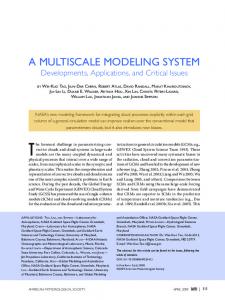
US Transplantation Data. This graph indicates the large disparity between the number of people waiting for an organ and the number of people that receive an organ. The data also indicates that the number of people that die while waiting is comparable to the number of people that receive a transplant. If we consider the trends in the data, it is obvious that the disparity between the number of people that require a transplant and the number of people that receive a transplant will continue to grow [2]. . . . . . . . . . . . . . . . . . . . . . . . . . . . . . . . . . . . . . . . . . . . . . . . . . . . . . . . . . . . . . . . . . . . . . . . . . . . . . . . . . . . . .
2
Computer Aided Tissue Engineering. This discipline uses and develops technologies for three key areas, Computer-Aided Tissue and Bio-Modeling, Scaffold Informatics and Biomimetic Design, and Bio-Manufacturing. . . . . . . . . . . . . . . . . . . . . . . . . . . . . . . . . . . . . . . . . . . . . . . . . . . . . . . . . . . . . . . . . . . . . . . . . . . .
4
2.3
Examples of SFF based fabrication systems. (a) Three-dimensional printing, (b) precision extrusion, and (c) multi-nozzle deposition . . . . . . . . . . . . . . . . . . . . . . . . . . . . . . . . . . . . . . . . . . . . . . . . . . . . . . . . . . . . . . 10
2.4
Overview of Scaffold Based Tissue Engineering. The process begins by extracting a tissue biopsy and placing cells from that biopsy into a cell suspension. Then a compatible material in fabricated into a 3D structure, a scaffold. The scaffold is then seeded with the cells and placed in a bioreactor for culturing. After culturing, a 3D functional tissue should form. . . . . . . . . . . . . . . . . . . . . . . 11
3.1
Multi-scale Modeling of a Bone Sample.The left column portrays identifying the damaged bone that requires replacement. The bone tissue can be studied at the micro-scale and the macro-scale. At the micro-scale, we can determine the bone’s morphology and quantify its properties. On the far right at the macro-scale, we can determine the loading conditions the bone experiences. We introduce a meso-scale to create a continuum between the micro- and macro-scales. It is at this level that the research introduces a unit-cell methodology for bone scaffold designs. . . . . . . . . . . . . . . . 15
3.2
Basic Premise of Unit Cell based Scaffolds. Tissue heterogeneity creates regions in the tissue with different properties like the ones depicted in this femur. If tissue engineering seeks to mimic a natural tissue, it must also generate structures that include this heterogeneity. Therefore, tissue engineering can develop smaller structure, unit cells, which are design for the local needs of specific cells. The unit cells can then be assemble together to meet the global needs of the entire tissue. . . . . . . . . . . . . . . . . . . . . . . . . . . . . . . . . . . . . . . . . . . . . . . . . . . . . . . . . . . . . . . . . . . . . . . . . . . . . . . . . . . . . . . . . . . . . . . . . . . . . 16
3.3
Key Components of Unit Cell based Scaffolds. Unit cell based scaffolds consists of four key components, unit cell design, unit cell characterization, unit cell assembly, and fabrication of the unit cell based scaffold. . . . . . . . . . . . . . . . . . . . . . . . . . . . . . . . . . . . . . . . . . . . . . . . . . . . . . . . . . . . . . . . . . . . . . . . . . . . . . . . . . . 19
3.4
Unit Cell. This figure gives a front view and an isometric view of the unit cell used in this case study. The mechanical properties for this unit cell structure was published by Sun et al. [56]. The structures were analyzed under increasing porosities and as 3 different materials. . . . . . . . . . . . . . . . . . . . 20
4.1
Two-Phase unit cell: Sample Two-Phase unit cell with the structural dimensions labeled the parameters listed describe the geometry of the unit cell features. The relationship between these parameters can be interrelated by the designer. . . . . . . . . . . . . . . . . . . . . . . . . . . . . . . . . . . . . . . . . . . . . . . . . . . . . . . . . . 27
4.2
Finite Element Analysis Method: Finite Element Analysis begins with constructing or importing a meshed geometry and defining its boundary conditions and applied loads, as depicted in (a). The applied form is uniform over a surface. In (b), the load is applied. In (c), the unit cell has been deformed and the stresses it experiences are depicted as contours [17] . . . . . . . . . . . . . . . . . . . . 32
ix
4.3
Procedure for Asymptotic Homogenization: This process can be utilized for determining the mechanical properties for a given unit cell design. First, a unit cell is meshed and material information and boundary conditions are entered. Next, the Stiffness Matrix, K and the Force Vector, f, are used to solve the Homogenization equation. This process computes the mechanical properties for one case. The process is repeated for 6 characterized directions xx, yy, zz, xy, xz, and yz and yields the effective mechanical properties for a region represented by this unit cell [17]. . . 33
4.4
Transport Properties Initial Conditions: Part of the input information for transport in STARCD [9]. Note, there are a number of properties which rely on both the fluid properties and the imposed flow conditions set by the designer. . . . . . . . . . . . . . . . . . . . . . . . . . . . . . . . . . . . . . . . . . . . . . . . . . . . . . . . . . . . 33
4.5
Computational Fluid Dynamics model of a fluid space: The geometry of the fluid space is created or imported into STAR-CD, such as in (a), and initial fluid conditions are defined for the space, as in (b). In (c), we see the resulting interior velocity contours that are produced from the geometry and initial conditions [9]. . . . . . . . . . . . . . . . . . . . . . . . . . . . . . . . . . . . . . . . . . . . . . . . . . . . . . . . . . . . . . . . . . . . . . 34
5.1
Assembly Process. . . . . . . . . . . . . . . . . . . . . . . . . . . . . . . . . . . . . . . . . . . . . . . . . . . . . . . . . . . . . . . . . . . . . . . . . . . . . . . . . . . . . . . 36
5.2
Unit cell properties may fall below and above the target value. The distance to from the target value to the unit-cell property is the target discrepancy. . . . . . . . . . . . . . . . . . . . . . . . . . . . . . . . . . . . . . . . . . . . . . . 37
5.3
Overview of Unit Cell Candidate Selection Process. The process begins with the characterized unit cell base and the characterized scaffold region. The properties of the unit cells are compared to the property ranges of the scaffold regions. Those unit cells with meet the property requirements form the unit cell candidate set. . . . . . . . . . . . . . . . . . . . . . . . . . . . . . . . . . . . . . . . . . . . . . . . . . . . . . . . . . 40
5.4
Overview of Unit Cell Candidate Ranking Process. Parameter Weights and the Unit Cell Candidate Set serve as the inputs for a given region. . . . . . . . . . . . . . . . . . . . . . . . . . . . . . . . . . . . . . . . . . . . . . . . . . . . . . . . . . 42
5.5
Unit Cell Properties above and below the target value. . . . . . . . . . . . . . . . . . . . . . . . . . . . . . . . . . . . . . . . . . . . . . . . . 43
5.6
Overview of the Unit-cell Alignment Method. Left: Unit-cells represented by skeletons. Middle: Transformation to simulate alignment. Right: Determination of alignment based on minimum Earth Mover’s Distance. . . . . . . . . . . . . . . . . . . . . . . . . . . . . . . . . . . . . . . . . . . . . . . . . . . . . . . . . . . . . . . . . . . . . . . . . . . . . . . . . 44
5.7
1D Connections: In each figure, there are two edges. On each edge, a phase for connection is indicated by the vertex, black point, and the radius, half circle, of the phase. Possible connections between the edges are indicated by shaded areas. The figure in part (a) has thinner connections than the figure in part (b). The size of the connection will determine if the connection is feasible and desirable for transport. . . . . . . . . . . . . . . . . . . . . . . . . . . . . . . . . . . . . . . . . . . . . . . . . . . . . . . . . . . . . . . . . . . . . . . . . . . . . . . 56
5.8
1D Connection Cases: In the first case, (a), the phase on the right is being aligned with the phase on the left. If the right phase’s upper outer-limit (V m − Rm) is able to align along any position between the upper and lower outer limits (V n − Rn and V n + Rn) then a connection is created. Similarly, in (b), the phase on the left is being aligned with the phase on the right. If the left phase’s upper outer-limit (V n − Rn) is able to align along any position between the upper and lower outer limits (V m − Rm and V m + Rn) then a connection is created. In (c), we have the case where the vertices of each phase align perfectly. . . . . . . . . . . . . . . . . . . . . . . . . . . . . . . . . . . . . . . . . . . . . . . . . . 56
x
5.9
1D Connection Size: The connection size for both conditions (a) and (b) is ((V m+Rm)−(V n− Rn)) and will be compared to a connection threshold value, α. If the connection size meets or exceeds the threshold, the alignment is considered as a potential alignment. If the connection size does not meet or exceed the threshold, a new alignment needs to be sought. . . . . . . . . . . . . . . . . . . . 57
5.10 2D Connectivity: 2D connectivity lets us align surfaces. In the example above, we have two surfaces with areas we wish to align. There can not be perfect alignment between these two surfaces. The relationship between the areas on each surface is different, making perfect alignment between the two surfaces impossible. This forces a search for the alignment that will yield connections that meet or exceed our threshold conditions. . . . . . . . . . . . . . . . . . . . . . . . . . . . . . . . . . . . . . . . . . . . 57 5.11 2D Connectivity Error: After alignment, the hatched areas which do not overlap constitute the error between the surface to surface matching. The error needs to be minimized, so that dead porosity does not increase within a unit-cell. . . . . . . . . . . . . . . . . . . . . . . . . . . . . . . . . . . . . . . . . . . . . . . . . . . . . . . . . . . . 58 5.12 Application Sample: In part (a), we see a connected figure, which was partially constructed out of the figures in parts (b) and (c). The figures in parts (b) and (c) were evaluated against the criterion set forth to determine the possible alignments to create connections for the shaded regions. 58 5.13 Skeleton visualization. a) Sample skeleton created for a simple 2D shape, b) Skeletonization process for skeleton points, which are positioned at the center of maximal circles (dashed lines), c) Complete set of skeleton points d) Enlarged view of portion of skeleton shows the actual skeleton points . . . . . . . . . . . . . . . . . . . . . . . . . . . . . . . . . . . . . . . . . . . . . . . . . . . . . . . . . . . . . . . . . . . . . . . . . . . . . . . . . . . . . . . . . . . 59 5.14 Comparing Effective Mechanical Properties by the Rule of Mixtures for Case 1. The combinations created in Case 1 are listed. The effective mechanical properties for each combination are given along with the difference from the target value and the percent error. Our highest ranked combination also has the least amount of error. . . . . . . . . . . . . . . . . . . . . . . . . . . . . . . . . . . . . . . . . . . . . . . . . . . . . . . . 64 5.15 Comparing Effective Mechanical Properties determined by the Rule of Mixtures and the Homogenization Theory with the relative error. The results for the elastic modulus, the shear modulus, and the Poisson’s Ratio are given in tables (a), (b), and (c), respectively. While the Homogenization Theory would be the more accurate, it is more labor intensive. This table shows that the Rule of Mixtures can be applied to narrow the search for unit cell combinations without such an intensive amount of labor while still using the Homogenization Theory to analyze the combinations.. . . . . . . . . . . . . . . . . . . . . . . . . . . . . . . . . . . . . . . . . . . . . . . . . . . . . . . . . . . . . . . . . . . . . . . . . . . . . . . . . . . . . . . . . . . . . 65 6.1
Volumetric Design Process Overview. The process includes collecting data from the damaged tissue, gathering the biological and processing considerations for the specific application and fabrication process, designing the underlying topology using a Steiner Tree, calculating an optimized cross section, and sweeping that cross section across the trajectory path to form a fully connected 3D scaffold.. . . . . . . . . . . . . . . . . . . . . . . . . . . . . . . . . . . . . . . . . . . . . . . . . . . . . . . . . . . . . . . . . . . . . . . . . . . . . . . . . . . 69
xi
6.2
Imposing an Underlying Structure. The damaged tissue will constitute the available space the tissue scaffold can occupy. The outer geometry of the space will be generated from the patient-specific anatomical data. We will assume the space is devoid of any solid structure per implantation procedures. One example of such a space is given in Figure a. We will assume the space has an imposed underlying structure. The underlying structure will define the set of points and edges from which we will construct our tissue scaffold. The underlying structure itself is constrained by the resolution limitations of the fabrication process. Therefore, a regular structure can be imposed on the space, such as the lattice in Figure b. We will also assume that the scaffold must interface with the natural tissue in order to integrate the regenerating tissue into the patient. Figure c. depicts connection points for this example as shaded spheres.. . . . . . . . . . . . . . . . . . . . . . . . . . . . . . 70
6.3
Generating a Tissue Scaffold. After defining the space, the underlying structure, and connection points, the wireframe of the structure will need to be generated. Generating the wireframe, or the Steiner tree, requires finding the minimal structure, composed entirely of a subset of the underlying structure, that will connect the connection points, without introducing cycles. In the process to form the wireframe, additional points from the underlying structure can be selected. These points are referred to as Steiner points, and an example is depicted in Figure a as shaded cubes. Through these Steiner points, it is possible to generate a structure that occupies both the outer wall and the interior space. The resulting structure, such as the one in Figure b, will be grown into a scaffold by sweeping optimized cross sections across the edges that connect the connection and Steiner points. The optimization will work to either minimize or maximize an objective function, which in this case is scaffold volume and which relies on biological, chemical, and mechanical scaffold requirements over time. One example of this volumetric growth is depicted in Figure c. . . . . . . . . . . . . . . . . . . . . . . . . . . . . . . . . . . . . . . . . . . . . . . . . . . . . . . . . . . . . . . . . . . . . . . . . . . . . . . . . . . . . . 70
6.4
2D Example of a Steiner Tree. In general, we will make an assumption, that there is an underlying structure to denote the distribution of all points and edges. For example, Figure a shows one possibility in which the space consists of regular lattice points in 2D. The connection points are highlighted in Figure b with shaded circles. These points are required to connect with the natural tissue and are a subset of the underlying structure. To establish the wireframe, we may add additional Steiner points from the underlying structure. Figure c denotes the Steiner points as shaded squares. The Steiner tree establishes a connected minimal structure formed by the required points, Steiner points, and their associated edges. The resulting structure is depicted in Figure d. . . . . . . . . . . . . . . . . . . . . . . . . . . . . . . . . . . . . . . . . . . . . . . . . . . . . . . . . . . . . . . . . . . . . . . . . . . . . . . . . . . . . . . . . . . . . . . . . . . 72
6.5
Comparison between Minimum Spanning Tree and Steiner Tree. Given a set of four points, the minimum spanning tree will result in the structure on the left. The Steiner tree will include two additional points and will result in the structure on the right. . . . . . . . . . . . . . . . . . . . . . . . . . . . . . . . . . . . . . 72
6.6
Determining the length of the tree generated . . . . . . . . . . . . . . . . . . . . . . . . . . . . . . . . . . . . . . . . . . . . . . . . . . . . . . . 72
6.7
Comparing the Minimum Spanning Tree and the Steiner Tree. The equation comparing the lengths for the Minimum Spanning tree and the Steiner tree is given in Equation 6.4. The equation is simplified until the inequality is subject to only one variable, as given in Equation 6.8. By plotting Equation 6.8 over a range of 0◦ ≤ α ≤ 90◦ , the range for which Equation 6.8 is true can be determined. Therefore, if 37◦ ≤ α ≤ 90◦ then the length of the Steiner tree is less than the length of the length of the minimum spanning tree. . . . . . . . . . . . . . . . . . . . . . . . . . . . . . . . . . . . . . . . . . . 74
6.8
Determination of connection point. This is an example of applying the skeletonization process the exterior and the interior of a femur head. . . . . . . . . . . . . . . . . . . . . . . . . . . . . . . . . . . . . . . . . . . . . . . . . . . . . . . . . . . . 80
xii
6.9
Trajectory Paths in CAD Software. Current CAD software is capable of using swept volumes to design parts. In the figure, Wildfire ProEngineering 3.0 is used to create a swept volume. The process begins by generating a trajectory path, that has a defined start and stop. Next, a cross section is sketched at the start point. The cross section in this figure is constant but there are options within the software to also produce variable cross sections. The software produces a preview of the part. At this stage options like thin wall and remove material can be selected . Finally, the swept volume is generated. . . . . . . . . . . . . . . . . . . . . . . . . . . . . . . . . . . . . . . . . . . . . . . . . . . . . . . . . . . . . . . . . . 81
6.10 Possible Cross Sections . . . . . . . . . . . . . . . . . . . . . . . . . . . . . . . . . . . . . . . . . . . . . . . . . . . . . . . . . . . . . . . . . . . . . . . . . . . . . . . . . . 82 7.1
Initial connection points.These are the initial to the case study. The coordinates of the points are (0,0,0), (0,3,0),(2.4,0,0), and (2.4,3,0). To generate a single layer design, all the connection points have the same z coordinate value. . . . . . . . . . . . . . . . . . . . . . . . . . . . . . . . . . . . . . . . . . . . . . . . . . . . . . . . . . . . . . . . 87
7.2
Imposed Lattice. This lattice has an equal spacing of 0.2 mm and contains all the vertices and edges for the trajectory path. . . . . . . . . . . . . . . . . . . . . . . . . . . . . . . . . . . . . . . . . . . . . . . . . . . . . . . . . . . . . . . . . . . . . . . . . . . . . 88
7.3
Trajectory Paths. The two trajectory paths are based on the same four initial connection points. The path in (a) has a length of 9.8mm and the path in (b) has a length of 10.2mm. . . . . . . . . . . . . . . . . . . 88
7.4
Single Layer Unit Cell using Struts. These samples were generated using the same trajectory path. Sample (a) was generated to have a porosity of 60%, while sample (b) was generated to have a porosity of 80%. . . . . . . . . . . . . . . . . . . . . . . . . . . . . . . . . . . . . . . . . . . . . . . . . . . . . . . . . . . . . . . . . . . . . . . . . . . . . . . . . . . 89
7.5
Samples with Square Cross Sections All four samples have a square cross section. Both samples (a) and (b) have porosities of 60%, while samples (c) and (d) have porosities of 80%. . . . . . . . . . 90
7.6
Mass Properties for Trajectory 1 based Designs. These are the mass properties obtained from ProE for the 9.8 mm long trajectory path, which includes the volume of scale material present in the design. The volume values have been circled and are given below each readout as well as the total volume. The actual porosity and the error, based on these results, is also given for each. . . . . . . 90
7.7
Mass Properties for Trajectory 1 based Designs. These are the mass properties obtained from ProE for the 10.2 mm long trajectory path, which includes the volume of scale material present in the design. The volume values have been circled and are given below each readout as well as the total volume. The actual porosity and the error, based on these results, is also given for each.. . 91
7.8
Source of Geometrical Error. The trajectory paths for these two structures are equal in length and are denoted by the dotted lines. . . . . . . . . . . . . . . . . . . . . . . . . . . . . . . . . . . . . . . . . . . . . . . . . . . . . . . . . . . . . . . . . . . . . . 91
7.9
Mesh for FEA of a 60% Porous Structure. This structure was meshed in ANSYS. It uses SOLID185 tetrahedra as the element type, contains 1402 nodes, and 4844 elements. . . . . . . . . . . . . . . . 93
7.10 Mesh for FEA of a 60% Porous Structure. This structure was meshed in ANSYS. It uses SOLID185 tetrahedra as the element type, contains 1968 nodes, and 7039 elements. . . . . . . . . . . . . . . . 94 7.11 Applied Displacements and Constraints on a Designed Unit Cell Layer. The displacement has been applied in the x direction in (a), the y direction in (b), and the z direction in (c). . . . . . . . . . 94 7.12 Displacement Contour Plot. This structure experienced a displacement of 0.003 mm in the x direction. This is a plot of the displacement experienced by the structure with a strain of 0.001 in the x direction. . . . . . . . . . . . . . . . . . . . . . . . . . . . . . . . . . . . . . . . . . . . . . . . . . . . . . . . . . . . . . . . . . . . . . . . . . . . . . . . . . . . . . . . . . . . 96
xiii
7.13 Displacement Contour Plot. This structure experienced a displacement of 0.0027 mm in the y direction. This is a plot of the displacement experienced by the structure with a strain of 0.001 in the y direction. . . . . . . . . . . . . . . . . . . . . . . . . . . . . . . . . . . . . . . . . . . . . . . . . . . . . . . . . . . . . . . . . . . . . . . . . . . . . . . . . . . . . . . . . . . . 96 7.14 Stress Contour Plot. Under a strain of 0.001 in the x direction, this structure experienced a maximum stress of 5.680 MPa and an average stress of 2.327 MPa. . . . . . . . . . . . . . . . . . . . . . . . . . . . . . . . . . . 97 7.15 Stress Contour Plot. Under a strain of 0.001 in the x direction, this structure experienced a maximum stress of 1.676 MPa and an average stress of 0.434 MPa. . . . . . . . . . . . . . . . . . . . . . . . . . . . . . . . . . . 97 7.16 Stress Contour Plot. Under a strain of 0.001 in the z direction, this structure experienced a maximum stress and average stress of 4.1 MPa.. . . . . . . . . . . . . . . . . . . . . . . . . . . . . . . . . . . . . . . . . . . . . . . . . . . . . . . . 98 7.17 Displacement Contour Plot. This structure experienced a displacement of 0.003 mm in the x direction. This is plot of the displacement experienced by the structure with a strain of 0.001 in the x direction. . . . . . . . . . . . . . . . . . . . . . . . . . . . . . . . . . . . . . . . . . . . . . . . . . . . . . . . . . . . . . . . . . . . . . . . . . . . . . . . . . . . . . . . . . . . 99 7.18 Stress Contour Plot. Under a strain of 0.001 in the x direction, this structure experienced a maximum stress of 4.465 MPa.. . . . . . . . . . . . . . . . . . . . . . . . . . . . . . . . . . . . . . . . . . . . . . . . . . . . . . . . . . . . . . . . . . . . . . . . . . 99 7.19 Stress Contour Plot. Under a strain of 0.001 in the y direction, this structure experienced a maximum stress of 2.687 MPa.. . . . . . . . . . . . . . . . . . . . . . . . . . . . . . . . . . . . . . . . . . . . . . . . . . . . . . . . . . . . . . . . . . . . . . . . . . 100 7.20 Stress Contour Plot. Contour plot of the stresses experienced by the structure with a strain of 0.001 in the z direction. . . . . . . . . . . . . . . . . . . . . . . . . . . . . . . . . . . . . . . . . . . . . . . . . . . . . . . . . . . . . . . . . . . . . . . . . . . . . . . . . . . 100 7.21 Multilayer Design. The multilayer design uses the first single later design, where the design is repeated with a 90◦ turn. . . . . . . . . . . . . . . . . . . . . . . . . . . . . . . . . . . . . . . . . . . . . . . . . . . . . . . . . . . . . . . . . . . . . . . . . . . . . . . . . . 100 7.22 Multilayer Mesh. This structure was meshed in ANSYS. It uses SOLID185 tetrahedra as the element type, contains 458 nodes, and 1193 elements. . . . . . . . . . . . . . . . . . . . . . . . . . . . . . . . . . . . . . . . . . . . . . . . . 101 7.23 Displacement Contour Plot in x direction. . . . . . . . . . . . . . . . . . . . . . . . . . . . . . . . . . . . . . . . . . . . . . . . . . . . . . . . . . . . . . . 101 7.24 Displacement Contour Plot in z direction . . . . . . . . . . . . . . . . . . . . . . . . . . . . . . . . . . . . . . . . . . . . . . . . . . . . . . . . . . . . . . . 102 7.25 Stress Contour Plot in the x direction . . . . . . . . . . . . . . . . . . . . . . . . . . . . . . . . . . . . . . . . . . . . . . . . . . . . . . . . . . . . . . . . . . . 102 7.26 Stress Contour Plot in the z direction . . . . . . . . . . . . . . . . . . . . . . . . . . . . . . . . . . . . . . . . . . . . . . . . . . . . . . . . . . . . . . . . . . . 102 7.27 Example of A 3D VST Based Unit Cell. Unlike the previous designs, this design began with connection points that lie on more than one plane. The resulting trajectory path as well as the calculated cross section are presented. This path and cross section result in a fully connected 3D design. . . . . . . . . . . . . . . . . . . . . . . . . . . . . . . . . . . . . . . . . . . . . . . . . . . . . . . . . . . . . . . . . . . . . . . . . . . . . . . . . . . . . . . . . . . . . . . . . . . . 103 7.28 Unit Cell ExamplesThese two examples show that the resulting design can be controlled by the unit cell designer. The first design delivers a unit cell that is essentially a piece of bulk material. The second design has incorporated symmetry by starting with symmetrical connection points. . . . 103
xiv
When we are honest with ourselves, we must admit that our lives are all that really belong to us. So it is how we use our lives that determined what kind of men we are. It is my deepest belief that only by giving of our lives do we find life. – Cesar Chavez (1927 - 1993) American activist and labor leader
xv
Abstract A Unit Cell Based Multi-scale Modeling and Design Approach for Tissue Engineered Scaffolds Connie Gomez Advisor: Wei Sun, PhD & Ali Shokoufandeh, PhD
”‘Tissue engineering is the application of principles and methods of engineering and life sciences toward the fundamental understanding of structure-function relationships in normal and pathological mammalian tissues and the development of biological substitutes to restore, maintain, or improve tissue function”’ [35]. One key component to tissue engineering is using three dimensional (3D) porous scaffolds to guide cells during the regeneration process. These scaffolds are intended to provide cells with an environment that promotes cell attachment, proliferation, and differentiation. After sufficient tissue regeneration using in-vitro culturing methods, the scaffold/tissue structure is implanted into the patient, where the scaffold will degrade away, thereby leaving only regenerated tissue. The need to design these scaffold structures and the need for precision control during fabrication have lead to numerous challenges as well as to the development of the field of Computer Aided Tissue Engineering (CATE). CATE currently employs the application of computer aided technologies which have been tools within engineering and non-invasive medical imaging, namely, computer-aided design (CAD), computer-aided manufacturing (CAM), solid freeform fabrication (SFF), computed tomography (CT) and magnetic resonance imaging (MRI) for modeling, designing, and manufacturing man-made tissue replacements. Current CATE technologies are capable of producing intricate scaffolds with a great deal of control. Through the addition of existing tools from the field of computer science, the time required to design these intricate scaffolds and assess their ability to meet numerous design parameters can be greatly decreased. This thesis reports research that develops tools to further the abilities of tissue engineers to generate and fabricate biomimetic scaffold designs efficiently. The major accomplishments reported in this thesis include: 1. Development of a framework of a unit cell based systematic approach for tissue scaffold design, including a unit cell informatics and property characterization crossing the unit cell structural scale levels based on the major design parameters. 2. The establishment of criteria between 1D and 2D geometries for creating either material continuity or fluid pathway connectivity between unit cells within a scaffold. 3. The development of an algorithm that will assemble unit cells such that within a tissue scaffold, unit
xvi
cells are matched to specific regions based on design requirements and there is connectivity between adjacent regions. 4. The development of a novel unit cell design approach, Volumetric Steiner Tree (VST), based on maintaining the underlying topology and therefore the connectivity of the unit cell. These novel approaches for modeling, designing and fabricating heterogeneous patient specific are possible by integrating existing computer science tools with existing CATE technologies. This research will also enable tissue engineers and cell biologists to expedite scaffold based tissue engineering research by minimizing the amount of human intervention required to design and fabricate either a heterogeneous scaffold with connectivity or a scaffold with prescribed design requirements.
1
2. INTRODUCTION
2.1
Tissue Engineering Tissue engineering seeks to replace or repair damaged tissues and organs by applying fundamental knowl-
edge from the fields of medicine, life sciences, and engineering to develop biocompatible substitutes that will restore functionality to a tissue [35]. This field has arisen due to the limitations of medicine today. Even with the modern advances in medicine and science, the standard medical procedure to replace or repair damaged tissues and organs is still either transplantation, which is donor dependent, or the use of an implant. While there are three possible types of grafts for transplantation, autografts, allografts, and xenografts, all three types of grafts have major disadvantages and all fall short of meeting the need for replacement tissues, which by 2000 has already resulted in approximately 1,000,000 surgical procedures a year in the US alone [1]. In the case of autografts, the replacement tissue is taken from the patient and is used to replace the damaged tissue. By using the body’s own tissue, the risk of tissue rejection is eliminated. Due to the body’s ability to accept this type of graft, it is considered the gold standard in transplantation. The fact that the tissue is taken from the patient presents several problems; this procedure can only remove a limited amount of tissue and will leave the patient with additional morbidity sites which further stresses the body during the tissue regeneration process. Allografts use tissue or organs from another person. Using a graft from someone else eliminates the need for additional morbidity sites, but introduces the the risk of immune rejection. Patients must therefore stay on a regimen of immune suppressants for the remainder of their lives, making them more susceptible to other illnesses. Unlike autografts, allografts can encompass much larger amounts of tissue and tissue types in a single donation. The alarming fact however is the disparity between the number of people that require a donation and the number of donors. Figure 2.1 gives the number of donors, the number of people on the waiting list, and the number of people that die while waiting for a donation in the US over the past few years. It is obvious from this data that there exists an increasing gap between donors and patients. It is this gap that tissue engineering is trying to close. Xenografts are grafts taken from a different species to serve as the replacement tissue and which are much more plentiful than human donors. However, the risk of rejection and the risk of infection is greatly increased due the introduction of such a foreign tissue into the human body. Implants on the other hand can reestablish tissue functionality without necessarily regenerating the tissue
2
Figure 2.1: US Transplantation Data. This graph indicates the large disparity between the number of people waiting for an organ and the number of people that receive an organ. The data also indicates that the number of people that die while waiting is comparable to the number of people that receive a transplant. If we consider the trends in the data, it is obvious that the disparity between the number of people that require a transplant and the number of people that receive a transplant will continue to grow [2].
3
but will generate a host of other issues. Since implants are permanent structures, the tissue around the implant will undergo atrophy over time, leading to replacement implants. The process of replacing an implant can only be repeated one to two times in most cases. For younger patients, this means there may come a day when a replacement implant is no longer possible. For older patients, the risks involved in the surgery increase significantly due to their age, which only continues to increase with each replacement. One of the central tissue engineering concepts is the use of scaffolds to guide the overall shape of the tissue and the differentiation of multiple cell types to produce a heterogeneous tissue [36]. Fundamentally, tissue engineering seeks to culture a sample of a patient’s cells within a scaffold that promotes cell and tissue growth and implant the new tissue growth into the damaged organ to restore functionality. Like autografts, the use of the patient’s own cells eliminates the risk of immune rejection from the body. Like allografts and xenografts, acquiring the ability to culture the cells outside the body provides a much larger potential source of tissue. However unlike implants, the support structures intended for tissue engineering applications are not meant to be permanent. Currently, there have been only a few successes within tissue engineering, but all of them have been achieved using a scaffold. Researchers have succeeded in growing human skin [14], non load bearing cartilage [48], and human urinary bladders [6]. These milestones reinforce the possibility of growing organs such as bone, liver, and heart valves for clinical applications within the next few decades. Additionally, the research that has been conducted in the disciple of tissue engineering has lead to the development of two key areas of interest Computer Aided Tissue Engineering and Scaffold Guided Tissue Engineering.
2.2
Computer Aided Tissue Engineering Computer Aided Tissue Engineering (CATE) encompasses the enabling technologies that can supply
anatomical data to the tissue engineer, that can permit design and analysis of tissue scaffolds and regenerated tissue, and that fabricate scaffold designs. Some of the enabling technologies included in CATE are computer aided design (CAD), computer aided manufacturing (CAM), rapid prototyping (RP), solid freeform fabrication (SFF), and image processing. The growth of this field is due in part to the recent advances in both software and hardware. Figure 2.2 gives an overview of the three areas within CATE, 1) computer aided tissue and bio-modeling, 2) scaffold informatics and biomimetic design, and 3) bio-fabrication. While all three areas will be discussed in this work, the primary focus will be on the first two areas.
4
Figure 2.2: Computer Aided Tissue Engineering. This discipline uses and develops technologies for three key areas, Computer-Aided Tissue and Bio-Modeling, Scaffold Informatics and Biomimetic Design, and Bio-Manufacturing.
5
2.2.1
Computer Aided Tissue Modeling
This first area of CATE begins with the premise that evolution has optimized the human physiology and it is this physiology that tissue engineers should try to approach. Therefore any attempt to model this physiology first requires gathering as much data from anatomical data to serve as our starting point. Typically, this involves obtaining non-invasive images of the body through computed tomography (CT) and magnetic resonance imaging (MRI) technologies. CT and MRI perform multiple scans on the body, producing a series of 2D cross sectional images of the body. These images can be morphed to form 3D models of either the entire tissue or just the region of interest for diagnosis, surgical planning, implant design, and tissue engineering [56, 28]. While the outer geometry of the natural tissue can be determined, this area allows for the manipulation of information to generate patient specific scaffold structures. This is also in the area of CATE that tissue engineers can introduce heterogeneous structures through the use of architecture and/or the use of multiple materials.
2.2.2
Computer Aided Tissue Informatics
This second area of CATE has developed due to the large quantities of information that can be currently gathered from natural tissue and from scaffolds. This area is crucial to providing tissue engineers with classification procedures, efficient retrieval of properties, studies, and any other pertinent information. This area depends heavily of computational algorithms and statistical tools and analytical tools. By developing both the tools and the algorithms, tissue engineers can pinpoint data without being overwhelmed by the amount of data. In fact, pinpointing data allows tissue engineers to incorporate their findings into the scaffold design parameters and to tailor a design to a specific application. It is this portion of CATE that can greatly benefit from the integration of existing tools found in the discipline of computer science.
2.2.3
Computer Aided Tissue Manufacturing
The intricate nature of scaffold designs and the scale on which that fabrication must take place requires the use of computer aided manufacturing technologies. The application of these to tissue engineering has opened up the field of scaffold guided tissue engineering as well as the development of new fabrication systems. Due to the need for controlled manufacturing of scaffolds, CATE has applied rapid prototyping (RP) techniques, principally solid freeform fabrication (SFF) technologies to fabricating tissue constructs, which constitutes the third area of CATE. SFF systems can link CAD software, typically used for the design of
6
the scaffold, to a fabrication facility. SFF systems use an additive approach to fabrication. In a typical SFF process the CAD model is sliced into layers, the designs in each layer are converted to machine instructions, and each layer of the CAD model is printed on top of each other one at a time. These fabrication processes are typically used to make prototypes for industry. Over the past few years, tissue engineers have utilized SFF technology for the fabrication of interconnected intricate scaffolds which a high degree of reproducibility using multiple materials [5, 61]. These are the qualities which have made SFF processes attractive to tissue engineering applications. There are currently a number of available SFF processes, some of which are illustrated in Figure 2.3, such as 3D Printing (3DPT M ) [24], fused deposition [29], and micro-nozzle extrusion systems [32]. 3DPT M was developed at MIT [11] and was based on the concept of a desktop printer. The process begins by laying down an even layer of powder in one powder bed. Then a print head drops a binder material onto the powder layer according to the given design. When the binder material and the powder touch, their particles bond with each other. Then another even layer of powder is laid down. This process is repeated until the entire model is completed. After wards, the model is excavated from the powder bed and dusted off. Fused deposition feeds filaments of thermoplastic biomaterial through a set of rollers into a chamber where the filament is melted. The melted thermoplastic is then extruded through a nozzle to form stands. The strands are built up in a layer by layer method. Micro-nozzle extrusion systems are capable of processing hydrogels, which is an attractive material type for soft tissue scaffolds and drug delivery systems. These systems couple pneumatic micro-valves and micronozzles to deposit strands of hydrogels [32].
2.3
Scaffold Based Tissue Engineering Scaffold guided tissue engineering is the use of a 3D construct to manipulate cells to regenerate into a
functional 3D tissue. The scaffold must perform both mechanical and biological functions. From a mechanical standpoint, the scaffold provides structural support to withstand applied forces and to mimic the mechanical signals experienced by the cell due to those applied loads. From a biological standpoint the scaffold promotes cell attachment in a 3D space, high surface areas and architecture that allows for cell proliferation, and pathways for the transfer of nutrients throughout the scaffold. As the tissue regenerates, the scaffold must also degrade away in order to have the applied forces solely on the regenerating tissue and to avoid any subsequent atrophy of the surrounding tissue.
7
2.3.1
Challenges in Scaffold Guided Tissue Engineering
The number of functions that the scaffold must accomplish during regeneration has lead to design and fabrication issues as tissue engineers attempt create a highly effective scaffold. The issues include material selection, designing cell specific micro-architecture with interconnectivity, developing methods to fabricate scaffolds, and synchronizing the scaffold to degrade and the same rate as tissue regeneration. The first issue is the selection of scaffold material. The material must be biocompatible if it is to serve as the environment for cells. It must also be biodegradable and not release products that adversely effect during degradation. If possible, it would be advantageous if the material was bioreabsorbable, so that at the end of the process, the scaffold material completely leaves the body. The second issue is designing or generating a micro-architecture that has porosity, pore size, and surface area that will promote cell growth of a specific cell type. The porosity and pore size will directly effect how the cells will differentiate, while the surface area will factor into the number of cells that are able to attach to the scaffold. The method and amount of design control is dependent on the fabrication process that will generate the scaffold. Consequently, the third issue facing scaffold guided tissue engineering is the development of fabrication processes. Scaffolds have been produced using various processes, such as gas foaming, salt leaching, freeze drying, electrospinning, and solid freeform fabrication [19, 28, 39, 13]. All of these processes are able to produce micro-architecture. The chemical based processes, gas foaming, salt leaching, and freeze drying, as well as electrospinning have an inherent randomness in their resulting structure, but have three major disadvantages. These processes rely on chemicals, which may remain in the scaffold and adversely affect cells, they have interconnectivity which can not be guaranteed due to the reliance on chemical reactions to form the tissue, and they are not reproducible. The fourth issue in scaffold guided tissue engineering is the synchronization between the scaffold’s degradation and the tissue’s regeneration. By transferring the applied forces from the scaffold to the regenerating tissue, the regenerating tissue is receiving larger and more realistic signals. It is the application of these signals to the tissue that will cause it to develop into a tissue with predefined functionality.
2.4
Research Objectives and Thesis Contributions The objective of this research is to develop a a unit cell based systematic and efficient approach to design,
characterize, assemble, and fabricate unit cell based tissue scaffolds through the use of computer aided tissue engineering. This thesis provides an overview of comprehensive engineering and computational paradigms
8
that have been brought together to address tissue scaffolds from bio-CAD modeling to scaffold fabrication. The contributions from this research will be detailed in the following sections.
2.4.1
Multi-scale Modeling and Design using a Unit Cell Structure
This thesis contributes two components vital for generating biomimetic scaffolds through multi-scale modeling, by presenting systematic approaches to obtaining data from the natural tissue and for incorporating that data into a scaffold. Due to the nature and function of biological systems, data that pertains to cellular growth as well as data that pertains to the structural function of the tissue in relation to the rest of the body must be gathered. Our contribution is a multi-scale approach to extracting data from anatomical sources and a unit-cell based approach to scaffold design that spans multiple scales and incorporates the extracted data.
2.4.2
Establishing Connectivity Criteria and Unit Cell Characterization
The thesis makes is a four-fold contribution from this area of tissue engineering. Firstly, the thesis establishes a set of criteria to determine whether connectivity is created after joining two unit cell faces together. Secondly, an alternative representation method is introduced to reduce the complexity while testing unit cells. Thirdly, the key parameters that effect unit cell performance are detailed along with the design considerations they impact. Lastly, a systematic approach to characterizing a unit cell is established.
2.4.3
Assembly Unit Cells into a Scaffold
This portion of the thesis makes two contributions to tissue engineering. It defines a selection process by which unit cells can be assembled into a scaffold that meets both local and global scaffold requirements. Furthermore, it presents a method to compare the multi-scale parameters of unit cell structures.
2.4.4
Topology based Unit Cell Design
In this portion of the thesis, the major contribution is the development of a unit cell design approach which is based on the structures underlying topology, that ensures a fully connected structure is generated. It combines three techniques Sweep Volume, Steiner Tree, and Primal-Dual optimization, to form a new approach called Volumetric Steiner Tree (VST). The VST results in the determination of the underlying topology for a fully connected structure, an optimized cross sectional area based on multiple design constraints, and the structure generated from sweeping the cross section along the underlying topology.
9
2.5
Thesis Outline This dissertation discusses each component in isolation and then reviews the performance and contribu-
tion of the component to the whole picture of tissue engineering. In Chapter 2, a multi-scale approach that extracts data from patient specific anatomical information and available literature as well as a unit cell based method to couple these pieces of data for the generation of a tissue scaffold are presented. Subsequently, in Chapter 3, the parameters to capture the data for the multi-scale design approach are set forth. Additionally, this chapter also presents the methods by which any given unit cell may be characterized using established engineering methods. Chapter 4 presents both the determination of connectivity between unit cells based on skeletal representations of the unit cells as well as the approach to assembly the unit cells together into a heterogeneous scaffold. Chapter 5 presents an approach to design a unit cell based on an underlying topology that needs to be maintained during the regeneration of the tissue, which has been named the Volumetric Steiner Tree. Chapter 6 presents an application of the Volumetric Steiner Tree to unit cell cell design. Chapter 7 includes summary, discussion, and conclusions about the research and its impact on scaffold based tissue engineering as well as recommendations for future work.
10
Figure 2.3: Examples of SFF based fabrication systems. (a) Three-dimensional printing, (b) precision extrusion, and (c) multi-nozzle deposition
11
Figure 2.4: Overview of Scaffold Based Tissue Engineering. The process begins by extracting a tissue biopsy and placing cells from that biopsy into a cell suspension. Then a compatible material in fabricated into a 3D structure, a scaffold. The scaffold is then seeded with the cells and placed in a bioreactor for culturing. After culturing, a 3D functional tissue should form.
12
3. Framework of A Unit Cell based Multi-scale Modeling Approach for Biomimetic Design
3.1
Introduction Scaffold guided tissue engineering is concerned with providing cells with an environment that produces
signals that will cause the cells to regenerate into a functional 3D tissue. This approach to tissue engineering has already successfully produced functional tissue, namely cartilage and portions of human bladder []. The signals a scaffold may deliver could be chemical, structural, or mechanical, in nature. Therefore some of the fundamental issues in tissue engineering include understanding the source for the various signals, identifying the effect of a particular signal on a cell, and incorporating those signals into scaffold design. It is clear from the broad spectrum of these issues, tissue engineering will also have to understand and mimic these signals on multiple scales within a 3D tissue scaffold. Subsequently, modeling tissue will have to begin from one scale and then be linked to other scales. Understanding, modeling, and manipulating the effect of one scale on another by linking those scales, is the ultimate goal of multi-scale approaches. Our multi-scale understanding of the tissue is further complicated by our view of tissue function. If the tissue is viewed as a chemical environment present on the micro-scale, tissue engineers can identify which materials promote cell attachment as well as materials that could lead to cell death. It is important to note that although there are various types of cells found in the body, classifying a material as biocompatible is dependent on the material’s effect on both the specific cell being regenerated and it effect to the rest of the body. If the tissue is viewed as a macro-scale structure, the architectural design and the mechanical properties can be mimicked through established engineering approaches, such as compression testing and finite element analysis, (FEA). The question for dealing with the tissue in this manner is how much of a sample is required for testing and analysis. From observation, it is understood that the tissue is under applied loading from daily movements. These applied forces clearly affect the entire tissue. Therefore, tissue engineers must utilize the information which is gathered from these techniques to model the structure and the mechanical properties which are seen by the cells. From these observations, it is clear that tissue engineers must consider conditions present at different scales as well as characteristics which span different criteria. In order to design a better scaffold, it is imperative that tissue engineering establishes a design approach which bridges multiple scales and identifies the key parameters which are affecting local cellular behavior. The introduction of a meso-scale as an intermediate
13
layer glues the micro- and macro-scales and more importantly provides a platform on which to conduct tissue scaffold design that can incorporate known information from both the micro- and macro-scales.
3.2
Multi-scale Characteristics of Bone Tissue Due to the structures present in biological systems, there is a need for modeling tissue at multiple scales,
also called multi-scale modeling, to gain insight into issues such as drug delivery, drug interaction, gene expression and cellular-environment interactions [49]. All of which have a direct bearing on successfully regenerating a functional 3D tissue. Applying a multi-scale modeling approach to biological systems will form a continuum between extreme scales, which will allow tissue engineers to understand the propagation of effects stemming from an alternation perform on one scale. This approach is already being applied to bridge nano- and micro-scales as well as micro- and macro-scales within various research areas in tissue engineering [47]. Among the most prominent systems in the body is the skeletal system, which is composed of bone and cartilage. At the macro-scale, it provides structural support, protects the body’s vital organs, and even defines a person’s range of motion [53]. The bone itself is a heterogeneous in nature, comprised of two distinct sections, compact bone and trabecular bone [53]. At the micro-scale, the differences in compact and trabecular bone become apparent. Compact bone, much as the name suggests, is a dense outer layer while the trabecular bone is a spongy secondary layer [53]. Additionally, all of the bones within the skeletal system are constantly being remodeled allowing the body to redistribute material to areas according to mechanical and chemical signals. This thesis bridges the micro- and macro-scales through the introduction of a meso-scale, which lies between the micro- and macro-scales. By introducing this scale, it provides tissue engineers with a platform onto which they can design scaffolds and which can serve to translate the signals incurred on one scale onto another.
3.2.1
Micro-Scale Characteristics of Bone
The morphology or micro-architecture of bone as well as the bone surface can be seen using current Scanning Electron Microscopy (SEM) technology. Although the architecture appears random, each bone type there are several types of substructures or features which are repeated. For example, the calcified struts in trabecular bone allow for open spaces and give the tissue its spongy quality [25]. While current technologies can capture images of the bone, the computational cost of capturing enough information and producing an
14
exact 3D reconstruction of the micro-scale architecture for large samples exceeds current technological limits. However, these images can provide pore size and porosity data. In addition to the tissue structure, it is at the micro-scale where we can model the interaction between cells, namely osteoblasts and osteocytes, and their environment [33]. However, the connection between an applied load to the bone and the mechanical signal a cell receives is not completely understood.
3.2.2
Macro-Scale Characteristics of Bone
As previously mentioned, bones provide structural support to the body during daily movements. Those movements apply forces on the bone and serve as the initiating mechanical signals to the body during bone remodeling. In the face of greater forces being applied, the bone generates greater amount of compact bone at the location where those forces are applied. One example of this occurs in the femural head. The head experiences large forces as it supports the upper body and high impact forces incurred during walking. The head is composed mostly of compact bone, which has a higher elastic modulus than trabecular bone. The elastic properties and the anatomical geometry can be generated using imaging technologies, such as Magnetic Resonance Imaging (MRI), and micro-Computed Tomography(micro-CT). These images can be used to quantify the structural and mechanical properties of the tissue through a Quantitative Computed Tomography (QCT) [45] and homogenization approaches [28]. This distribution of compact and trabecular bone make bones heterogeneous structures.
3.2.3
The Meso-scale
To bridge the micro- and macro-scales and to produce a heterogeneous scaffold, a meso-scale or middle scale is presented such that it will incorporate the data gathered from the micro- and macro-scales. The introduction of this meso-scale is the premise underlying the unit cell based methodology and a major contribution of this thesis. The meso-scale is the platform on which the morphological, structural, and mechanical properties of the tissue, and the loading conditions for the tissue location will be used to design a heterogeneous scaffold. The meso-scale model will incorporate this information into a unit cell design that will bridge the micro-scale and the macro-scale. The advantage of introducing this scale is that changes to the micro-scale can be linked to changes in the meso-scale, which can subsequently be linked to changes in the macro-scale, thereby forming a continuum between the scales. The application of this method is clearly illustrated in Figure 3.1. The process begins by identifying the damaged bone that requires replacement. At the micro-scale, the bone’s micro-architecture and morphology can be examined and its mechanical properties can be quantified. Likewise at the macro-scale, we can de-
15
Figure 3.1: Multi-scale Modeling of a Bone Sample.The left column portrays identifying the damaged bone that requires replacement. The bone tissue can be studied at the micro-scale and the macro-scale. At the micro-scale, we can determine the bone’s morphology and quantify its properties. On the far right at the macro-scale, we can determine the loading conditions the bone experiences. We introduce a meso-scale to create a continuum between the micro- and macro-scales. It is at this level that the research introduces a unit-cell methodology for bone scaffold designs.
termine the loading conditions the bone experiences. We introduce a meso-scale that creates a continuum between the micro- and macro-scales. At this level we introduce a unit cell methodology for bone scaffold designs. The unit cell design must then incorporate the architectural requirements from the micro-scale and the mechanical properties from the macro-scale.
3.3
Unit Cell based Scaffolds This part of the research contributes an application of unit cell based design approach to tissue scaffolds,
in particular bone tissue scaffolds. A unit cell is the basic design that is repeated to form a pattern and that can be used within the heterogeneous scaffold [17]. The properties of the unit cell are equivalent to the properties of an assembly of those unit cells. A unit cell design will fill an anatomical geometry, which is obtained from patient data about the damage tissue. Due to the heterogeneity of the tissue, there are regions in the tissue
16
Figure 3.2: Basic Premise of Unit Cell based Scaffolds. Tissue heterogeneity creates regions in the tissue with different properties like the ones depicted in this femur. If tissue engineering seeks to mimic a natural tissue, it must also generate structures that include this heterogeneity. Therefore, tissue engineering can develop smaller structure, unit cells, which are design for the local needs of specific cells. The unit cells can then be assemble together to meet the global needs of the entire tissue.
that will require different unit cells. The overall approach to unit cell based scaffold design is illustrated in Figure 3.2. This approach is attractive to tissue engineering because it reduces the complexity of designing and fabricating an optimized structure with both micro- and macro- scale features. This approach is also attractive because of it applicability to generating heterogeneous structures, by joining two different unit cell structures. Subsequently the need for different unit cells requires a system for organizing the unit cells and any associated information. Therefore a unit-cell library will be compiled to contain unit-cell designs and their information for scaffold assembly and fabrication.
3.3.1
Unit Cell Design
Individual unit-cell design focuses a specific cell type and the material and micro-architecture preferences of the cell type. The scaffold material must allow for cell attachment and must not adversely affect the
17
cell as the scaffold degrades. Due to the limited number of biocompatible material approved by the USDA, researchers are currently attempting to create biocompatible composites for scaffolds that increase mechanical function as well as cell interaction [26, 38]. The micro-architecture has several quantifiable parameters such as porosity, pore size, and surface areas. From the tissue morphology, the repeating of feature types such as rods and struts also form part of the microarchitecture. The specific parameters and features must lay within the upper and lower limits determined for a specific cell. The overall dimensions of the unit cell also need to be considered as part of the microarchitecture for this process. While the unit cells will form a repeating structure to fill the volume, the unit cell based approach deals principally with a single unit cell during scaffold design. For this reason, this thesis uses sets for a standard size of a 1 mm x 1 mm x 1mm volume in which the unit cell is designed. There have been several methods for designing unit cells, namely Equivalent morphology, Stochastic modeling, Voroni modeling, and the method presented by this thesis Volumetric Steiner Tree. Equivalent morphology bases the predominant micro-architecture features such as rods, on the predominant features in the natural tissue. Stochastic modeling and Voroni modeling mimic the randomness found in the natural tissue into their designs. The Volumetric Steiner Tree method utilizes the structure’s underlying topology to form a fully connected structure with an optimized geometry.
3.3.2
Unit Cell Characterization
While unit cells can be designed using any number of methods, the resulting structure must ultimately meet the requirements of the region to which they will be assigned. Therefore, this research sets forth a set of computational and engineering based approaches to evaluate the unit-cell properties. By applying these approaches to any unit cell design, the properties of the unit-cells can be used for comparison to the tissue and evaluation as a scaffold.
3.3.3
Unit Cell Assembly
One of the key issues in unit cell based approaches is assembling the unit such that the interface between the different unit cells does not cause a sharp discontinuity. Having a discontinuity in the scaffold could result in a point of area of high stress concentration which could lead to fracture. Additionally, it pathways are not maintained between the different unit cells then the flow of nutrients is impeded or halted completely, and essentially starving the cells. Therefore any assembly method must insure meeting local constraints of the regions and adequate connectivity between the unit cells for flow as well as connections that will not fracture.
18
3.3.4
Fabrication of a Unit Cell based Scaffold
The SSF based fabrication of a unit cell based scaffold has already been developed by our laboratory. However it relies on knowing the unit cells that will be used prior to fabrication. The process requires the data be prepared manually for each scaffold design. By extending the characterization process and by standardizing our unit cells, this research lays the foundation to automate this process, thereby reducing the time from design to fabrication even further.
3.4
Case Study In the case of the femur head given in Figure 3.2, there is information from both the micro- and macro-
scale. From the micro-scale, architecture for bone should have a porosity between 65 % to 75 % and a pore size from 200 microns to 400 microns. From the macro-scale, the effective elastic modulus of different regions was calculated for seven distinct layers. By establishing the meso-scale for a unit cell design, the parameters from the micro-scale and the macroscale can be achieved. In this study, a prescribed architecture was used and is depicted in Figure 3.4. This structure was analyzed under 3 different materials and a range of porosities by Sun et al. [56]. The elastic moduli for these structures are given in Figure 3.2. This study considers Layer 1 and Layer 2 of the femur head. Layer 1 requires an elastic modulus of 0.62 GPa and Layer 2 requires an elastic modulus of 0.71 GPa. From the reported elastic moduli, Layer 1 and Layer 2 can be constructed using poly-L-lactic acid (L-PLA) with 70 % and 66 % porosities respectively. The porosity of the unit cell structures can be determined using the follow equation [56].
P =N×
� � �� � � f f 1 L × l2 × − − 1 × l3 × 2 × 3 2 2 L
(3.1)
where P is the porosity of the unit cell, L is the length of the unit cell, l is the pore size, f is the number of faces with pores, and N is the number of pores on a face. In the case of this unit cell, the length of the structure is 1 mm, there are 6 faces with pores, and there are 4 pores on each face. The equation can be reduced as follows,
19
20
Figure 3.4: Unit Cell. This figure gives a front view and an isometric view of the unit cell used in this case study. The mechanical properties for this unit cell structure was published by Sun et al. [56]. The structures were analyzed under increasing porosities and as 3 different materials.
21
P =4×
�� � � � � 6 6 1 × l2 × − − 1 × l3 × 2 2 2 � 2 � � P = 4 × l × 3 − (3 − 1) × l3 × 2 � � � P = 4 × l2 × 3 − 4 × l3 P = 12 × l2 − 16 × l3
(3.2) (3.3) (3.4) (3.5)
Using this equation to obtain the required porosities, the unit cell for Layer 1 should have a 300 micron pore size and unit cell for Layer 2 should have a 325 micron pore size. Therefore, for Layers 1 and 2, there are unit cell designs, depicted in Figure 3.2 and scaffold material selections. It is clear from this case that scaffolds can be designed by focusing on the unit cell at the meso-scale with requirements from the microand macro-scales.
3.5
Conclusions This part of the research contributes the introduction of a meso-scale that ties the micro- and the macro-
scales into a continuum. This new scale fills in the gap between cellular needs, such as architecture and porosity, and externally applied forces. Furthermore, this scale provides tissue engineers with a platform on which to design scaffolds. Additionally, this thesis identifies a method of working in the meso-scale by introducing a unit cell based scaffold design method for tissue scaffolds. This method focuses on designing a non repeating structure, a unit cell, that conforms to micro-scale and whose mechanical properties match those of a structure constructed by repeating the unit cell structure several hundreds of times. This research also presents preliminary unit cell designs based solely on porosity, pore size, mechanical properties, and material selection, which illustrates the ability to use the meso-scale for unit cell design. It depicts how the micro-scale requirements and the macro-scale requirements will be tied to the meso-scale during unit cell design. It also depicts how the design method can use existing engineering technology and tools, such as finite element analysis, CAD software packages, and 3D reconstruction techniques. The presented case study also depicts the three major steps in unit cell design, acquiring data from the tissue at the micro- and macro-scales, acquiring data about the unit cells being considered, and matching the unit cell properties to the tissue requirements.
22
4. Unit Cell Informatics and Unit Cell Characterization
4.1
Introduction As demonstrated by the case study given in Section 3.4, there are three major steps involved in unit
cell design, 1) gathering data from the damaged tissue, 2) gathering data from the unit cell structures under consideration, and 3) matching the unit cells to a region in the tissue. The data from natural tissue will be patient specific and will require a 3D reconstruction and analysis prior to any selection of a unit cell design. Therefore, tissue engineers can begin this process by gathering information from their own unit cell designs that can be used in the later matching process. This portion of the thesis will focus on gathering data from unit cell structures in a systematic procedure. It will define a set of parameters that will account for all the unit cell design considerations and define the methods by which the unit cells can be characterized. Since this work takes place on the meso-scale, the characterization can be accomplished using established engineering techniques, such as finite element analysis [17].
4.2
Defining Unit Cell Criteria Designing environments that promote cell growth under normal loading conditions require insight into
the environment we are trying to mimic, namely a naturally occurring heterogeneous tissue. Therefore it is essential that the target tissue environment be analyzed and its properties used in subsequent unit cell scaffold designs. The information gathered from the tissue includes geometry, function, cells present, cell configuration, fluid properties and loading conditions. This work will define a set of critical unit cell parameters for the aforementioned properties.
4.2.1
Unit Cell Design Considerations
Tissue scaffolds and subsequently unit cells are designed to meet various considerations, listed in Table 4.1. Also listed in Table 4.1 are possible design selections, which can alter a unit cell’s properties. Many of the parameters describing the possible design selections are important to several areas. This creates an interdependence between possible design selections and unit cell properties. This aspect of tissue scaffold design means that the design approach will be required to evaluate unit cells based on multiple factors.
23 Design Consideration Mechanical • scaffold structural integrity • internal architectural stability • scaffold strength and stiffness Biological • cell loading, distribution, and nutrition • cell attachment and growth • cell-tissue aggregation and formation Geometric • anatomical fitting Transport • nutrient and oxygen delivery • waste removal • growth factor and drug delivery Fabrication • temperate ranges during process • control • resolution
Possible Selections Affecting Property • biomaterial selection • internal architecture • porosity and pore distribution • fabrication method • layout • pore size and interconnectivity • vasculature • scaffold external geometry • interconnectivity • permeability selection
• process parameters • materials
Table 4.1: Design Considerations: On the left, the design considerations for tissue scaffolds are divided into five groups. Each group has particular needs it must address. In the right column, the selection options that directly impact the needs being addressed in one or more groups.
Mechanical Design Considerations From the Table 4.1, we know that mechanical properties include structural integrity, architectural stability, strength and stiffness. These mechanical requirements are determined using mechanical testing or the QCT approach for a given location within the natural tissue. To meet those requirements, the unit cell will need to be constructed such that its effective Young’s Modulus, EEf f , in each direction is equivalent to the tissue under consideration. The EEf f in turn is dependent on the Young’s Modulus, E, of the bulk material and the geometry of the given unit cell [30]. Likewise, the other mechanical properties of effective shear stress, GEf f , and Poisson’s Ratio, ν, will depend on the properties of the scaffold material and the geometry [30]. However, it should be noted that the list of materials available for tissue scaffold applications is limited by the need for biocompatiblitiy and biodegradability of materials. The biological needs of the seeded cell will also dictate the geometry a unit cell in terms of porosity, φ, pore size, dpore , and pore area, Apore , [28]. The tissue under consideration is able to function within a limited space under variable temperature conditions, as a result we need to gather information concerning the density, ρ, and the thermal expansion coefficient, α. While these parameters have been related to mechanical properties due to global loading, they are also
24
important to other areas due to cellular needs [8, 31].
Biological Design Considerations The biological requirements, which are dictated by the desired tissue and are cell specific, include cell loading, distribution, attachment, proliferation, and tissue formation [55]. The biological requirements start with identifying the cell which will seed the scaffold and the medium which will support cell growth. The selection of the cell and medium will also eliminate some of the possible materials. Scaffold material selection is based on the cell’s ability to attach to the material and the medium’s reaction to the material. The cell selection will also determine the interior architecture in terms of porosity, φpore , pore size, dpore , pore area, Apore , and pore angles, θpore . These parameters are directly correlated to cellular behavior [57]. For a given cell, its biological requirements also extend to the flow patterns and conditions that must exist for a cell to attach to the unit cell surface and to receive adequate amounts of nutrients and growth factors. Currently, cell preferences are not completely known, but they must be identified as completely as possible with the prospect that they will yield information crucial to successful tissue growth [37].
Geometrical Design Considerations Geometry must be considered both at the macro-scale and at the meso-scale when examining the tissue. At the macro-scale, the overall anatomical geometry of the patient must be gathered and retained for later scaffold design. This information can be gathered from the patient via Computed Tomography (CT) or magnetic resonance imaging (MRI). These images undergo a reverse engineering process to reconstruct the outer geometry of the scaffold [55]. For the purposes of scaffold implants, the boundaries of the volume (regions of the scaffold) are constructed from the anatomical information gathered during the reverse engineering reconstruction. At the meso-scale, cell type and cell behavior will dictate the limitations of architectural features present. The tissue will also have a structural form which could also be mimicked in the unit cell design. For example, bone tends to have either rod or plate like structures, depending on their location in the body. The architectural information can be gathered in the form of parameters, such as length, l, and dimension relationships. As discussed in Section 4.2.1 geometrical relationships also directly affect transport properties.
Transport Design Considerations Since mass and fluid transport are essential for providing the cells with the materials needed to differentiate, the natural tissue can provide information on the fluid and the flow conditions for a given cell type.
25
Firstly, the fluid reaching the tissue has a density, ρf luid , and viscosity, µf luid . We also have the interior geometrical information, Apore , dpore , and φpore . Coupling this information with the geometric information already gathered and velocity, V , pressure, P , and temperature, T , the local flow conditions can be used to determine the Reynold’s number, Re, as in Equation 4.1, and therefore the type if flow present [10]. At the same time, fluid and mass transport through the tissue apply stresses on the tissue which affects cell behavior. This architecture insures that the tissue cells have the necessary nutrients for cell growth but also underlines the need to have interconnect fluid pathways [33].
Re =
4.2.2
ρf luid V dpore . µf luid
(4.1)
Fabrication Design Considerations
While the natural tissue can yield information needed to mimic an environment for cell growth, it is important to realize that current technologies can not reproduce the local geometries of natural tissues. For this reason, the limitations and the processes for scaffold fabrication need to be considered during scaffold design. Fabrication processes have limitations, such as feature size limits, material selection and the accuracy of its control system. These limitations must be considered when designing the unit cell architecture and aligning unit cells to form the overall scaffold. It is therefore important that assembly processes be able to take such matters into consideration. The process may also introduce temperature changes to the material during production.
4.2.3
Unit Cell Parameters
Heterogeneous tissue scaffold designs need to meet the design requirements of a particular application for biological requirements, material properties, structural properties, and transport parameters. The parameters for unit cell design and characterization constitute our set of unit cell informatics and are in Table 4.2. The unit cell-assembly methodology is in turn based on these parameters. The desired characteristics for a scaffold are dependent on the particular cell or cells to be cultured on the scaffold. While the optimal environments for culturing and co-culturing specific cells is still under investigation, unit cell characterization will provide scaffold designers information for unit cell selection once preferred environmental conditions are determined [51, 37].
26 Design Consideration Mechanical
Biological Geometric Transport Fabrication
Characterizing Parameter Exx , Eyy , Ezz , Gxy , Gyz , Gxz , υxy , υyz , υxz , Ef f Ef f Ef f f Ef f Ef f Exx , Eyy , Ezz , GEf xy , Gyz , Gxz , Ef f Ef f Ef f x y z υxy , υyz , υxz ,dpore , Apore , θpore , θpore , θpore ρ, α, φ x y z φsolid , φpore , dpore , Apore , θpore , θpore , θpore , x y z φsolid , φpore , dpore , Apore , θpore , θpore , θpore , l, h, w, r Re, ρf luid , µf luid , Apore , dpore , T , P , Vx , Vy , Vz , k, φsolid , φf luid T , l h, w, r
Table 4.2: Unit Cell Informatics: In the left column, design considerations are divided into five groups, mechanical, biological, geometric, transport, and fabrication. In the right column, the parameters that describe the material properties (Young’s Modulus, Shear Modulus, Poisson’s Ratio), fluid properties, geometry and scaffold conditions are listed. The material properties are for the xx, yy, zz, xy, xz, yz directions, both for the bulk material and effective material. Note, some of the parameters are in more than one location.
4.3
Geometrical Characterization The architecture of each unit cell is dependent on the tissue it is mimicking. While tissues can be similar,
their location in the body affects their internal architecture in order to handle the repeating loading conditions experienced at that location. For this reason, a unit cell can be designed to mimic the natural material. Designs include the use of rods and plates to mimic bone. This would allow unit cells to be classified by the architectural elements present in the unit cell. The specific geometry of each unit cell design will affect the mechanical properties and is critical for the fabrication process. Geometry determines the stress distributions within a structure and the maximum loading conditions a structure can withstand [15]. The geometry also determines the resolution requirements for the fabrication process. For our work, the geometry of a unit cell denotes the size and dimensions of the architectural features as in Figure 4.1. Structurally, the goal of scaffold designs is to mimic the mechanical and transport properties and the overall anatomical fit for future placement into the body. Prior work has used porosity and pore size as the basis for scaffold evaluation [61]. Pore size (dpore ) has been a parameter of most scaffold systems, and a large amount of research has been undertaken to create desired pore sizes repeatedly while using different fabrication processes [13, 28]. It is known that cells will only cross a specific spatial distances and obstacles in an environment. Cell movement limitations due to architecture are not completely understood but current evidence demonstrates cell behavior in the presence of different architecture can vary greatly [28]. The pore size is related to the pore shape and is denoted by both the area of the pore and the angles of the pore.
27
Figure 4.1: Two-Phase unit cell: Sample Two-Phase unit cell with the structural dimensions labeled the parameters listed describe the geometry of the unit cell features. The relationship between these parameters can be interrelated by the designer.
Efforts to mimic nature can lead to irregular pore shapes that make these parameters important to the unit cell structure characterization. Porosity, φf , is a critical parameter for characterization of scaffolds and is specific to the type of cell that will grow on the scaffold. Porosity is the fluid or contour-space volume-fraction of the unit cell. The porosity in a two-phase unit cell structure is the total volume of one phase over the total volume of the entire system. While this will yield the geometric porosity of the unit cell structure, the unit cell operating with fluid flowing through it will have an effective porosity. The effective porosity denotes how much of the available flow capacity is being used for flow through the unit cell. The ideal unit cell structure has an effective porosity equal to its geometric porosity, so that all areas within the unit cell structure that are in contact with the flow pathways. Areas where fluid does not flow are known as closed or dead porosity (φf c or φf d ). Dead porosity spaces are where cells have the least chance for survival or growth due to lack of available nutrients.
28
Each of the structural features has geometric dimensions, which are requirements during the fabrication process. A feature’s fabrication feasibility is limited only by the fabrication resolution. As in Figure 4.1, a unit cell will have features that have lengths, widths, heights, and angles (l, L, w, h, and θ). During characterization, that geometrical information will be recorded. The geometrical information will then be compared to the fabrication resolution. It will also be important to fluid flow through the unit cell, which is discussed in Sec.4.2.1.
4.4
Constitutive Characterization While it may seem obvious that each unit cell structure is at least a two phase system, it is important
to describe the constitutive properties of the phases present in a unit cell structure because of the impact the constitutive properties have on mechanical and on transport properties. This definition becomes more important as researches use multiple materials within a scaffold to generate heterogeneity. From the scaffold material, designers need at least the elastic modulus of bulk material, as well as the shear modulus, the Poisson’s ratio, and the coefficient of thermal expansion. This information is critical when determining the unit cells effective mechanical properties. From the fluid material, designers need at least the density, the viscosity, and diffusion constant. These properties are used when determining transport through a unit cell. While this research has considered only two phase unit cells, the ability to generate structures with multiple materials is a current technology [32] and the constitutive definition would encompass an additional set of material properties.
4.5
Mechanical Characterization The mechanical properties rely both on the material properties of the phase and the phase geometry. The
properties relating to the material need to consist of the standard 6 different directions,xx, yy, zz, xy, xz, and yz. The material properties needed for characterization include Young’s modulus, Eij , shear modulus, Gij , Poisson’s ratio, νij , and the coefficient of thermal expansion, α [30], where i and j range over x, y, and z. Different material choices have different bulk Young’s modulus, Eij , values. Therefore, material choice directly affects a scaffold’s ability to mimic the biological environment and for a given unit cell structure, the material will have a bulk Young’s modulus and an effective Young’s modulus. This does not fully characterize the unit cell in terms of scaffold material. The scaffold material’s surface affects cell attachment and fluid flow due to its surface roughness, e. Rougher surfaces decrease the velocity threshold that will produce turbulent flow [60]. The structural material also needs to be characterized by its effective
29 Ef f f Ef f Young’s modulus(Eij ), effective shear modulus, GEf . These material ij , and its Poisson’s ratio, νij
values are necessary to understand the structural material’s behavior when loaded under shear stresses and the effect that tensile loading will have on material along its length and across its width. The mechanical properties of a unit cell can be determined by one of the four methods: rule-of-mixtures, mechanical testing, finite element analysis (FEA), or a homogenization process [17].
4.5.1
Rule-of-Mixtures
Rule-of-Mixtures averages the properties of the materials found in the sample based on the volume fractions of each phase [30]. This leads to a linear relationship between porosity and effective elastic modulus, such as the relationship for the elastic modulus that presented in Eq 4.5.1. In mechanical testing, a sample is fitted with strain gages that measure deformation under stress. Then has a compressive force applied. The experimental strain data is used for mechanical property calculation. This method will yield experimental information but is time consuming due to the need for physical samples [17]. E1 = Ef V f + Em V m 4.5.2
Finite Element Analysis
The FEA method begins with the unit cell that has been meshed. Then one surface of the unit cell is held stationary while the opposite surface experiences an applied force. After the unit cell undergoes deformation, the amount of strain is reported. The boundary conditions (BC) and deformation for a unit cell undergoing this process in given in Figure 4.2. Using the known stress via the applied force, the surface area on which it was applied, and the reported strain values, the mechanical properties of the unit cell can be calculated using Hooke’s Law [20].
4.5.3
Homogenization Theory
Finally, a given unit cell of a region can undergo a homogenization process to determine its effective mechanical properties [17]. The unit cell will be treated as an anisotropic material, and therefore the Young’s modulus, the shear modulus and the Poisson’s ratio will be independent of each other. The process is presented in Figure 4.3. It begins by selecting unit cell for homogenization. Next, during the preprocessing phase, a mesh is created. The process then goes on to solve six characterized cases for the homogenization equation with inputs from the stiffness matrix, the boundary conditions, and the force vector. While it would be possible to use any of these methods, each comes with their own limitations. Both the FEA and homogenization approaches require a mesh of the unit cell design. If meshing is not possible,
30
then only the Rule-of-Mixtures can be used. If the number of nodes exceeds 2000, then both the FEA and the Rule-of-Mixtures can be used. Otherwise, all three methods are viable options for characterizing the unit cell.
4.6
Transport Characterization Similar to mechanical properties, fluid and mass transport rely on the fluid properties in the pore space
and the geometry of the unit cell. The transport properties also rely on the presence of any forced velocities or existing pressures. The addition or absence of an initial velocity or pressure determine whether the flow is forced or diffusion in nature [60]. Current modeling systems allow any initial velocity or pressure to be applied such as in Figure 4.4. Being able to apply an initial forced velocity, a unit cell is capable of experiencing different velocities, therefore different Reynold’s numbers and in turn both laminar and turbulent flow. This means that initial conditions for a given environment also need to be recorded. The components of properties such as velocity will be recorded using a Cartesian coordinate system. Similar to using different materials for the unit cell structure, different fluids inside the unit cell will affect the transport properties and flow conditions [33]. Each fluid has a viscosity, µ, a density, ρ and diffusion rate, κ, for a given temperature, T . These fluid properties are involved with determining the Reyonld’s number that affects the flow patterns present in the scaffold, the start of turbulence in a unit cell structure and what stresses a cell would undergo [60]. The flow patterns will also determine where mass will move through a scaffold. In order to mimic the environment in which the cells will grow,both the fluid properties and the conditions found either in nature or in a bioreactor need to be part of the design process for a unit cell structure and must be known for unit cell structure characterization. Also, the geometry has a direct affect on the Reynold’s number [60]. However, the geometrical information must be used in conjunction with the Re so that changes in flow due to geometry changes introduced through alignment can be limited. The combination of geometry, fluid properties and an initial velocity can be seen in Figure 4.5.
4.7
Conclusions In this chapter, the research focused on defining a systematic process to gather data from two phase unit
cell designs. The data gathered during process is vital to the entire unit cell based scaffold assembly because this data will be used to select unit cells for the different regions in a tissue. The first contribution in this chapter is defining a set of parameters that account for all the design considerations for a unit cell design. By defining these parameters, designers have quantifiable design parameters that
31
go beyond porosity and elastic modulus, as well as clear interrelationships between the design considerations, as indicated by the applicability of a parameter to multiple design considerations. Secondly, this chapter contributes a defined methodology for characterizing the unit cells and determining the values for the parameters set forth for unit cells. For some of the parameters, there are several characterization approaches that could apply, depending on the complexity of the unit cell design. It should be noted that all the characterization methods are well established approaches in engineering. These two contributions will form part of the initial data set for our unit cell design approach and is vital to generating a biomimetic tissue scaffold.
32
Figure 4.2: Finite Element Analysis Method: Finite Element Analysis begins with constructing or importing a meshed geometry and defining its boundary conditions and applied loads, as depicted in (a). The applied form is uniform over a surface. In (b), the load is applied. In (c), the unit cell has been deformed and the stresses it experiences are depicted as contours [17] .
33
Figure 4.3: Procedure for Asymptotic Homogenization: This process can be utilized for determining the mechanical properties for a given unit cell design. First, a unit cell is meshed and material information and boundary conditions are entered. Next, the Stiffness Matrix, K and the Force Vector, f, are used to solve the Homogenization equation. This process computes the mechanical properties for one case. The process is repeated for 6 characterized directions xx, yy, zz, xy, xz, and yz and yields the effective mechanical properties for a region represented by this unit cell [17].
Figure 4.4: Transport Properties Initial Conditions: Part of the input information for transport in STARCD [9]. Note, there are a number of properties which rely on both the fluid properties and the imposed flow conditions set by the designer.
34
Figure 4.5: Computational Fluid Dynamics model of a fluid space: The geometry of the fluid space is created or imported into STAR-CD, such as in (a), and initial fluid conditions are defined for the space, as in (b). In (c), we see the resulting interior velocity contours that are produced from the geometry and initial conditions [9].
35
5. Connectivity and Unit Cell Assembly
5.1
Introduction One of the major steps involved in unit cell based scaffold design is matching a unit cell to a region. While
this may seem simple, it actually poses a new problem, selecting unit cells that both match the requirements of the given region and generate available fluid pathways between regions. This is vital to the over all scaffold design for two reasons: 1) In order to generate a 3D tissue, the cells must be able to proliferate into the scaffold interior and 2) nutrients need pathways to reach the cells. This chapter of the thesis sets forth an algorithm to select unit cells for assembly and a set of connectivity criteria to be used to assembly the unit cells. To accomplish these goals, this chapter will also provide an alternative representation of the unit cell which is more conducive undergo the assembly process. To solve the problem of selecting unit cells for a given region that also construct pathways between unit cells, several pieces of information must be available, the unit cell informatics and the region requirements. The process for obtaining the unit cell informatics was covered in Chapter 3. There are several possible characterization processes for obtaining the requirements for the different regions in the natural tissue, such as computed tomography [45]. The overview of the algorithm is depicted in Figure 5.1.
5.2
Unit Cell Selection Each scaffold is patient specific and tailored to the individual’s needs. The scaffold’s outer geometry is
based on anatomical information from CT data and analyzed using MIMICS. The anatomical information ensures the physical fit of the scaffold into an in vivo environment. Further analysis of the naturally occurring tissue yields the mechanical properties. We then divided the scaffold volume into regions with similar mechanical properties. The goal is to determine which unit cell will be used for each region, where the unit cells should be placed, and what their orientation should be. Our approach to this problem is to first assume that a structure of one or more unit cells exists for a base region. This structure has a number of faces where unit cells are exposed, adjacent to a second region which needs to be filled. The goal is to find a suitable unit cell consistent with the requirements of the second region, and to determine the placement and orientation of this next unit cell on the existing structure. Our assumption of an existing base structure is not restrictive because the selection of a starting base unit cell is straightforward as will become apparent.
36
Figure 5.1: Assembly Process.
The algorithm for determining the placement and orientation of the next unit cell consists of several steps. The first step, Unit Cell Candidate Selection, which is described in Section 5.2.2 constructs a list of unit cells that may be suitable for a given region. These candidate unit cells are ordered according to a fitness function, with the most fit unit cell at the top of the list. The problem of choosing the base unit cell is solved by using the most fit unit cell. The unit cell candidates are then subjected to a ranking algorithm which is described in Section 5.2.4. This algorithm produces a ranking of the candidate cells with orientations.
5.2.1
Unit Cell Fitness
A scaffold region is characterized by a set of requirements, e.g. pore size, porosity, shear modulus etc. These requirements are determined during the characterization process [23]. The potentially large number of suitable unit-cells in a library indicates a need for a quantitative measure that can be used to discriminate among the various alternatives. We use the notion of a ranking or fitness function to rank-order candidate unit-cells. Higher fitness values correspond to better choices. Our fitness function uses concepts from the fields of multi-criteria optimization [16] and nonlinear multi-objective optimization [41]. The idea is to use a set of weights that control the relative importance of the requirement properties.
37
Figure 5.2: Unit cell properties may fall below and above the target value. The distance to from the target value to the unit-cell property is the target discrepancy.
For each of the requirement properties we obtain an upper bound, Hi , and lower bound, Li , on the range of acceptable values. The subscript i is an index into the list requirement properties, P . For example, we may want the pore size to be at least 0.1 (L1 = 0.1), and at most 0.3 (H1 = 0.3) millimeters, with the optimum target value in the middle of the range (0.2). These bounds are dictated by the application and the specific property. Intuitively, if any property is out of range the fitness of the unit cell is zero. For simplicity of presentation in this section we use the notation, F , to denote the fitness of a particular unit-cell. In the general case, fitness is determined for each unit-cell, i.e. Fu where u denotes the index of the unit-cell in the library. Similar notation is used for C which denotes a unit-cell’s property values, and D which denotes the distance from the target. As depicted in Figure 5.5, a unit-cell property may fall above or below the target value. For example, we can define the target, Ti for property i as the midpoint by
Ti
=
|Hi − Li | , 2
(5.1)
where Hi and Li are the upper and lower bounds, respectively. We can then define the normalized distance for a particular property, Di , between the target value, Ti , and the unit-cell property value, Ci as
Di
=
|Ti − Ci | . |Hi − Li |
(5.2)
We associate a weight, Wi , with each of the properties under consideration. The importance or weight of each property is a predetermined valued based on the scaffold application and is given as input [56]. We enforce a constraint on the weights,
38
|P | X
Wi = 1,
(5.3)
i=1
where Wi is the weighting for property i, and |P | is the number of properties under consideration. We argue that this constraint ensures that the relative fitness of separate regions is comparable. We can then formulate the fitness for a particular unit-cell, F as
F =
|P | X (0.5 − Di )Wi
if Li ≤ Ci ≤ Hi , i = 1, . . . , |P |
i=1
0
(5.4)
Otherwise.
In this way we can express the suitability of a unit-cell as a single number which indicates how well the unit-cell’s properties match the requirements for a specific region. The relative importance of individual properties can be modulated to suit the application, for example stiffness may be less important for nonload bearing scaffold regions. Additionally, properties can be assigned zero weights if they are not under consideration.
5.2.2
Unit Cell Candidate Selection
The goal of unit-cell candidate selection is to construct a list, ordered by fitness, of unit-cells suitable for a given region. The region is characterized by a set of requirements determined during the characterization process. We divide these requirements into two classes. The invariant requirements which are unaltered by rotation are shown in Table 5.1. The variant requirements are affected by rotation and are shown in Table 5.2. The construction of the list is straightforward. We take a set of weights for the invariant requirements subject to the constraint in Equation 5.3, determine the fitness, F , for each unit cell using Equation 5.4. We can then sort the list by fitness and eliminate unit-cells with fitness values of zero.
5.2.3
Unit Cell Alignment Algorithm
At this point, we have a set of unit cells with the invariant properties that satisfy the region ranges. The properties under consideration are below in Table 5.2. Again, there needs to be a comparison between the unit cell properties and those of the region. However, since the properties can change with a change of orientation, for a given unit cell, there may be orientations which meet the region properties and orientation which do not.
39 Invariant Structural Parameters Variable Description p The length across the pore o Pore space volume fraction a The area of a pore opening on a given plane e A measure the vertical deviations when traversing a surface Table 5.1: Invariant properties which do not change with rotation
Parameter Pore Size (µm) Porosity (%) Pore Area (µm2 ) Surface Roughness
Variant Parameters Parameter Variable Description Pressure s The force per unit area experienced by the fluid and scaffold Velocity in x direction (µm/s) x X component of velocity Velocity in y direction (µm/s) y Y component of velocity Velocity in z direction (µm/s) z Z component of velocity Elastic Modulus in x (GPa) E1 Bulk elastic modulus in x direction Elastic Modulus in y (GPa) E2 Bulk elastic modulus in y direction Elastic Modulus in z (GPa) E3 Bulk elastic modulus in z direction Poisson’s Ratio ν23 Poisson Ratio for y − z plane Poisson’s Ratio nu13 Poisson Ratio for x − z plane Poisson’s Ratio ν12 Poisson Ratio for x − y plane Shear Modulus (GPa) G23 Bulk shear modulus across the y-z plane Shear Modulus (GPa) G13 Bulk shear modulus across the x-z plane Shear Modulus (GPa) G12 Bulk shear modulus across the x-y plane Table 5.2: Variant properties which change with rotation
For this reason, a unit cell tested against the region’s properties must undergo rotation. While there are an infinite number of possible rotations, this approach uses discrete rotations to limit the time required for this step. The equations for this are below. The rotation of the unit cell is in terms of three angles, (θx , θy , θz ), each is about one axis. This procedure repeats for each property. There is a comparison between the unit cell properties and the region property ranges in two stages. The first stage involves the invariant unit cell properties, which are unaltered by rotation. The invariant properties consist of the unit cell’s geometric properties. If unit cell properties fall within the range of the invariant property ranges, the unit cell will pass to the second stage of unit cell selection. The equations that describe this step are also below.
40
Figure 5.3: Overview of Unit Cell Candidate Selection Process. The process begins with the characterized unit cell base and the characterized scaffold region. The properties of the unit cells are compared to the property ranges of the scaffold regions. Those unit cells with meet the property requirements form the unit cell candidate set.
I=
1
if Lp ≤ Cp ≤ Hp , Lo ≤ Cp ≤ Ho ,
La ≤ Cp ≤ Ha 0 Otherwise
41
where Ci is the property value, i, of the unit cell (i.e. Cp is pore size, p), Li is the lower bound on property value, i, of the unit cell, and Hi is the upper bound on property value, i, of the unit cell. At this point, we have a set of unit cells with the invariant properties that satisfy the region ranges. The properties under consideration are below in Table 5.2. Again, there needs to be a comparison between the unit cell properties and those of the region. However, since the properties can change with a change of orientation, for a given unit cell, there may be orientations which meet the region properties and orientation which do not. For this reason, a unit cell tested against the region’s properties must undergo rotation. While there are an infinite number of possible rotations, this approach uses discrete rotations to limit the time required for this step. The equations for this are below. The rotation of the unit cell is in terms of three angles, (θx , θy , θz ), each is about one axis. This procedure repeats for each property. However, obtaining the properties after rotation requires either an analysis or a calculation with assumptions. Due to the number of possible orientations and need for manual intervention, this approach uses the latter option. These calculations are later in the Rule of Mixtures Section. At this point, there should be a set of unit cells that have met the region’s property ranges. However, if our database does not contain any unit cells that meet both of these requirements, the process will require more unit cells in the database. Then the process will begin again. This cycle will continue unit there is at least one unit cell candidate. With the candidate unit cell selected, we can move to the next step of the process, which is orientation.
5.2.4
Ranking
After creating a candidate unit cell set, the candidate unit cells are ranked. By ranking the unit cells at this time, the unit cells with the properties closest to all the region properties can be used first during scaffold construction. Figure 5.4 gives an overview of the ranking process. The process has information from both the scaffold application and the unit cell database, which undergo three major steps for ranking. From the unit cell database, we have the properties of the unit cells. From the scaffold application, we have the property ranges for each region as well as the importance of each property for a given scaffold. The importance or weight of each property is a predetermined valued based on the scaffold application and is given as input values. The association between the weight and a property is given in Figure 5.4. As well as the weights for each property, the target value and the tolerance range for that parameter are inputs. The application dictates the target values for the parameters. However, meeting all the parameters of a region without specifically designing for that region means that the tolerances for each parameter allows consideration of the unit cells in the database for a region if they are close enough to the target value. The
42
Figure 5.4: Overview of Unit Cell Candidate Ranking Process. Parameter Weights and the Unit Cell Candidate Set serve as the inputs for a given region.
determination of what is close enough is dependent on both the application and the parameter. The upper and lower values of these tolerance ranges become the upper and lower bounds. As depicted in Figure 5.5, the unit cell property may fall below or above the target value. The difference between the target value and the unit cell value is the error. However since we are using multiple properties, the error has to become dimensionless and normalized. Since the unit cell property value has already been placed within the property range by the unit cell
43
Figure 5.5: Unit Cell Properties above and below the target value.
candidate selection, we know the unit cell value must be at or below the upper bound and at or above the lower bound. Finding the difference between the unit cell property and both bounds yields two values. The minimum value between the two is taken. This step is repeated to for each property. The equation for this step is
D1
= min(Cp − Lp , Hp − Cp )
D2
= min(Co − Lo , Ho − Co )
D3
= min(Ca − La , Ha − Ca )
D4
= min(Cs − Ls , Hs − Cs )
D5
= min(Cx − Lx , Hx − Cx )
D6
= min(Cy − Ly , Hy − Cy )
D7
= min(Cz − Lz , Hz − Cz ),
where Dn is the deviation associated with property n, Ci is the value of property i, Li is the lower bound for property i, and Hi is the upper bound for property i. While a deviation might be larger for one property than the other properties, this would not necessarily reduce a unit cell potential as a candidate. The weights, which are inputs, are the factors used to determine the effect of the deviation on the overall deviation. The sum of the weights equals one. Therefore, the properties with a higher importance have a corresponding higher weight value than the other properties. In this way, the properties of higher importance would need smaller amounts of deviations from the target value. After the weighted deviations are calculated, the overall error brought on by these deviations is calculated. To keep the effect of the deviations normalized across the properties, the weighted deviations are subtracted
44
from the number of properties used for this process. Therefore, the number of properties is flexible and dependent on the available information. The equations calculating the weighted deviations and the error for all the properties are, We can then formulate the fitness for a particular unit cell, i as
Si
=
|P | X
Wj Di,j
j=1
and the error as
Ei
= |P | − Si
where |P | X
Wj = 1,
j=1
Wi is the weighting for property i, and |P | is the number of properties under consideration. Once the error for each unit cell is calculated, the unit cells are ready for ranking. Unit cells with a lower error value are higher in the ranking. This ranking will determine the testing order of unit cells for a given region.
5.2.5
Alignment algorithm
Figure 5.6: Overview of the Unit-cell Alignment Method. Left: Unit-cells represented by skeletons. Middle: Transformation to simulate alignment. Right: Determination of alignment based on minimum Earth Mover’s Distance.
45
In order to incorporate unit-cell connectivity into our method, we need to determine the optimal orientation of adjacent unit-cells. The purpose of this process is to ensure pathways for flow to biological cells dispersed throughout the scaffold. We accomplish this through the use of skeleton-representations of the unit cells. Intuitively, we align the skeletons to achieve the best connectivity. Given a set of skeleton points, the Earth Mover’s Distance (EMD) framework [46] is applied to find an optimal match between the distributions. The EMD approach computes the minimum amount of work (defined in terms of displacements of the masses associated with points) it takes to transform one distribution into another. The Earth Mover’s Distance (EMD) is designed to evaluate dissimilarity between two multi-dimensional distributions. The EMD approach assumes that a distance measure between single features, called the ground distance, is given. In our approach, we use the Euclidean distance between skeletal points as the ground distance. The EMD then lifts this distance from individual features to full distributions. Moreover, if the weights of distributions are the same, and the ground distance is a metric, EMD induces a metric distance. However, the main advantage of using EMD lies in the fact that it permits partial matches in a natural way. This important property allows the similarity measure to deal with uneven clusters and noisy datasets. Computing the EMD is based on a solution to the well-known transportation problem [3] whose optimal value determines the minimum amount of work required to transform one distribution into the other. The skeletons are rotated through a discrete set of angles and the EMD is calculated for each rotation. The rotation with the lowest EMD corresponds to the orientation with the best flow connectivity. When unit cells are rotated to ensure flow connectivity, the mechanical properties of the unit-cells are affected. The fitness of the unit cells must be recalculated using the new property values generated by their new orientations. Determining the unit-cell properties after rotation is based on the Rule of Mixtures and is described in the following section.
5.3
Determining Mechanical Properties Using the Rule-of-Mixtures Tissue engineered scaffolds need to meet both the biological goals of tissue formation and the stresses
and loading conditions present in the human body. For this reason any design approach must insure that the mechanical properties of the resulting scaffold structure can withstand the loading conditions the scaffold is expected to experience. Our previous unit cell selection and alignment processes gave us a set of unit cells and their orientations that promotes fluid transport between regions. These region combinations will result in the creation of a heterogeneous tissue scaffold. As the regions are combined, the effective mechanical
46
properties of the overall scaffold will change. For this reason, we include determining mechanical properties in our algorithm. Our algorithm needs to evaluate the effective mechanical properties of the regions we fill as well as the effective mechanical properties of the combined regions. If the properties of two combined regions are similar to the properties of the two regions they are mimicking, the unit-cells and their orientations will be kept and the tissue scaffold will continue to grow by another region. If that particular combination does not yield mechanical properties similar to the original, then a new unit-cell, a new orientation, or both will be selected for a region and this process will continue until a combination is found, which yields effective mechanical properties similar to the desired mechanical properties. We determine effective mechanical properties by one of four approaches, compression testing, Asymptotic Homogenization Theory, Finite Element Analysis (FEA) or Rule-of-Mixtures [17]. The effective mechanical properties of a single region represented by a unit-cell may undergo a rotation that would require the properties to be recalculated. Similarly, combining regions will also change the effective mechanical properties of the overall scaffold [30]. For these reasons, we need to include the ability for mechanical property recalculation within our algorithm. The first three approaches are time consuming and labor intensive to complete given the number of combinations which are possible. These approaches include tasks such as creating a mesh which does not exceed a nodal limit and entering bulk material properties would be required for each possible combination [17, 56]. Unlike these approaches, the Rule-of-Mixtures approach can be integrated into the algorithm without using human labor during the combinatorial processes and can yield the effective mechanical properties of our structures. The Rule-of-Mixtures approach, as mentioned previously, is a well defined approach. It has been used for decades in the area of composite materials in order to consider the properties of fiber-reinforced composite laminates [30]. In fact, the equations for a laminate composed of two materials have been derived over 30 years ago [30]. Using this approach, the effective properties of the laminates could be determined. The following sections apply the Rule-of-Mixtures approach to unit cells, which are two-phase structures consisting of a biodegradable material and a fluid.
5.3.1
Assumptions
Unit cells may undergo alterations, such as rotation or cutting, which in turn means that its mechanical properties may need to be recalculated. To determine the effective properties of a tissue scaffold unit cell the following assumptions about the scaffold material have been made.
47
1. The material is isotropic. 2. The material or the pore space must be uni-directional in each layer of the unit cell. 3. The amount of strain in direction 1 (The x-direction) is the same for both the scaffold material and the pore space. It is also assumed that we know the following about each unit-cell. This information is gathered during the unit cell characterization and the information is stored in the unit cell database. 1. Porosity (o) = (Volume fraction of fluid pore space (V f )
2. Volume fraction of scaffold material (V m )
3. Pore Area (af )
4. Scaffold Area(am )
5. Pore orientation with respect to the global coordinate system(θ)
6. Density ρ =
5.3.2
�
mass of unit cell volume of unit cell
�
=
�
mass of unit cell (1−length of pore×P ore Area)
�
Rule of Mixtures
Once these assumptions have been made, we can begin finding the mechanical properties of our structures. The Rule-of-Mixtures approach averages the mechanical properties of the different components or phases found in a structure. We are only considering two phases in each unit-cell, scaffold material and fluid space. Also, each unit-cell may use a different scaffold material, thereby allowing for the construction of a heterogeneous scaffold in terms of both structure and material. We are looking for the Effective Elastic Ef f f Ef f (Young’s) Modulus (Eij ), the Effective Shear Modulus (GEf ). ij ), and the Effective Poisson’s Ratio (νij
This approach averages the mechanical properties of the different components or phases found in a particular material. At this point, we are only considering two phases in each unit cell, scaffold material and fluid space. It is important to note that each unit cell may use a different scaffold material, thereby allowing
48
for the construction of a tissue scaffold that is heterogeneous scaffold in terms of both structure and material. The details of determining the mechanical properties for a single unit are given in the following sections.
Determination of E1 (The Elastic Modulus in the x-direction) Since the unit cell has two phases, the fluid pore space and the scaffold material, the effective elastic modulus will be determined based on the behavior of these two phases. Using the assumption that the pore space and the scaffold material undergo the same amount of deformation (�1 = �f1 = �m 1 ) and stress strains relationships for each phase, the effective elastic modulus for direction 1 can be calculated. Using the relationship between stress and strain the following two equations are known about the two phases. σ1f
= E1f �f1
(5.5)
σ1m
= E1m �m 1
(5.6)
Furthermore, using the relationship between stress, force and area, the following is also known. F1f F1m
= σ1f af = E1f �f1 af
(5.7)
m = σ1m am = E1f �m 1 a
σ1
=
σ1
=
σ1
=
F1f af
F1m am
+ + !
F1f
(5.8) F1m
+ A � m� f F1 F1 + A A ! ! E1f �f1 ∗ am E1f �f1 ∗ af + A A =
(5.9) (5.10) (5.11)
49
Using our assumption, the following can be said about the strain experienced by this material.
�
= �f1 = �m 1
�1 �
σ1 epsilon1 � f� a A � m� a A
= E1 =
E1 Vm
(5.12) E1f af
!
A
+
!
A
(5.13)
= Vf
(5.14)
= Vm
(5.15)
= E1f V f + E1m V m
(5.16)
1−Vf
=
= E1f V f + E1m 1 − V
E1
E1f am
(5.17) � f
(5.18)
This relationship is further simplified by recalling the fluid has an elastic modulus of zero
� E1 = E1m 1 − V f = E1m (1 − o) .
(5.19)
Determination of E2 (The Elastic Modulus in the y-direction) It is assumed that any stress that is applied to the unit cell is applied to both the fluid pore space and the scaffold material (σ2 = σ2f = σ2m ). Using these assumptions and the stress strain relations we can calculate the effective elastic modulus in direction 2. It is also important to note the distance between is denoted by (W ) with the change in that distance (∆W )and is composed of the changes in the distance for the scaffold material (∆W m ) and the pore area (∆W f ).
�f
=
�m
=
∆W �2 �2
σ2
! (5.20)
E2f �
σ2 E2m
� (5.21)
= �2 W = �f W f + �m W m
(5.22)
= �f V f + �m V m ! � � σ2 σ2 f Vm = V + m f E E2 2
(5.23) (5.24)
50
Then by dividing both sides by the constant stress, �
�
1 E2
�
1 E2
�
1
=
! Vf +
E2f 1
=
E2f
! f
�
�
V +
1 E2m
�
1 E2m
�
Vm
(5.25)
(1 − V f )
(5.26)
Since the elasticity of the fluid is zero the equation reduces to �
1 E2
�
� 1 (1 − V f ) E2m � � � � E2m E2m = = (1 − V f ) (1 − o) �
=
E2
(5.27) (5.28)
Determination of υ12 (Poisson’s Ratio) This property is obtained under the assumption that σ1 = σ. Transverse deformation is given as (∆w).
ν12
= −
�2 �1
(5.29)
∆w
f = −W �2 = −W ν12 �1 = ∆m w + ∆w
(5.30)
∆m w
= W V m ν m �1
(5.31)
∆fw
= W V f ν f �1
(5.32)
ν12
= νmV m + νf V f
(5.33)
Since our system is dominated by the scaffold material the following simplification is made
ν12 = ν m V m = ν m (1 − V f ) = ν m (1 − o)
(5.34)
Determination of G12 (Shear Modulus) It is assumed that the shear stresses (τ = τ f = τ m ) on both phases is equal. Therefore, by definition the following is true. Furthermore, the total deformation ∆ is composed of the material deformation (∆m ) and pore space deformation (∆f ).
51
=
γf
=
γ
=
∆
= γW = ∆m + ∆f
(5.38)
∆m
= V mW γm
(5.39)
∆f
= V f W γf
(5.40)
= V mγm + V f γf
(5.41)
= V mγm + V f γf
(5.42)
γ �
�
τ G12 � � τ G12 � � 1 G12
5.3.3
τ Gm τ Gf τ G12
γm
(5.35) (5.36) (5.37)
� τ � � τ � +Vf = Vm m G Gf � m� � f � V V = + Gm Gf
G12
=
G12
=
(5.43) (5.44)
Gm Gf V + V f Gm Gm G f (1 − o)Gf + oGm
(5.45)
m Gf
(5.46)
Stiffness Matrix Cij
This matrix consists of 36 elements. However the assumption that the material is isotropic reduces the number of independent elements to 2. C11 C12 C 12 C11 C12 C12 C= 0 0 0 0 0 0
C12 C12
0
0
0
0
0
0
C11
0
0
0
0
(C11 −C12 ) 2
0
0
0
0
(C11 −C12 ) 2
0
0
0
0
(C11 −C12 ) 2
The Stiff Matrix relates to the stress and the strain via the relationship given below.
52 σ 1 C11 σ C 2 12 σ3 C12 = τ23 0 τ 0 31 τ12 0
� 1 � 2 �3 γ23 γ 31 γ12
C12
C12
0
0
0
C11
C12
0
0
0
C12
C11
0
0
0
0
0
(C11 −C12 ) 2
0
0
0
0
0
(C11 −C12 ) 2
0
0
0
0
0
(C11 −C12 ) 2
This relationship can also be viewed as 0 0 0 � 1 S11 S12 S12 � S 0 0 0 2 12 S11 S23 0 0 0 �3 S12 S23 S11 = γ23 0 0 0 2 (S11 − S12 ) 0 0 γ 0 0 0 0 2 (S11 − S12 ) 0 31 0 0 0 0 0 2 (S11 − S12 ) γ12 S11 S 12 S12 Sij = 0 0 0
S12
S12
0
0
S11
S23
0
0
S23
S11
0
0
0
0
S44
0
0
0
0
S55
0
0
0
0
σ 1 σ 2 σ3 τ23 τ 31 τ12
0 0 0 0 0 S55
Due to the assumptions made at the beginning of this problem, this material can be considered to be isotropic. Also, to reduce the complexity of the problem, this first section will only consider strain in a plane. Later this will be expanded to include strain in two planes. Once that has been said, the components of the Sij and the
53
Cij can be given as, � S11
=
S12
=
S22
=
S23
=
S44
=
S55
=
C11
=
C12
=
C22
=
C23
=
C44
=
C55
=
S
5.3.4
� 1 E1 � � −ν12 E1 � � 1 E2 � � −ν23 E2 � � � � 1 2 (1 + ν23 ) = G23 E2 � � 1 G12 � � S22 S22 − S23 S23 S � � S12 S23 − S12 S22 S � � S22 S11 − S12 S12 S � � S12 S12 − S23 S11 S � � 1 S44 � � 1 S55
(5.47) (5.48) (5.49) (5.50) (5.51) (5.52) (5.53) (5.54) (5.55) (5.56) (5.57) (5.58)
= S11 S22 S22 − S11 S23 S23 − S22 S12 S12 + 2S12 S23 S12
(5.59)
Transformation
Since the direction of the pore space and may not align to direction 1, 2, or 3 the mechanical properties can be determined for the unit cell if the direction (angle θ is the angle between the x-direction and the 1direction) is known.
σx σ y τxy
σ1 −1 = [T ] σ 2 τ12
σx σ y τxy
=
2
cos θ 2
2
sin θ 2
sin θ
cos θ
sin θ cos θ
− sin θ cos θ
To reduce the transformation matrix(T ) to symbols
−2 sin θ cos θ σ1 2 sin θ cos θ σ2 cos2 θ − sin2 θ τ12
54
2 m 2 T = n −nm
2
m 2 T = n nm 0
n2 2
m
nm n
2
m2 −nm
2nm −2nm 2 2 m −n −2nm 2nm m2 − n 2
For a rotation, the S matrix, and consequently the C matrix will change. This means that the resulting matrix is in terms of the material properties, the porosity of the unit cell and the angle θ . This also means that the materials properties at that rotation can be calculated from the resulting matrix.
5.4
Connectivity Criteria Cells need nutrients, growth factors and waste disposal, making mass and fluid transport vital to cell
survival. To provide these factors to seeded cells, the fluid must have a pathway to and from the cells. As a result, our unit-cell methodology requires connected pathways between unit-cells. We use the pore-space topology to describe a unit-cell’s pathways. We in turn can use topological connectivity to establish a set of criterion to create connections between unit-cells. Prior to developing a set of criterion, we must first consider what is a connection between two-phase structures in 1D and 2D and what is connectivity. A connection is created when one phase of a structure is aligned with any amount of its corresponding phase in the second structure. A structure’s connectivity is the degree to which a structure can be cut before creating two distinct structures [43]. We used a progressive approach to establish the criteria starting from 1D and then extending it to 2D and 3D. The criteria was developed by first looking at 1D alignments (edge-to-edge) and then moving to 2D alignments (surface-to-surface). Connectivity within structures for 1D and 2D structures has been studied [50]. We represented the possible connections in a form that will allow unit-cells to be tested against the connection criteria developed. For that, we turned to skeleton representation. To utilize skeletal representation for selecting structures to be matched, criteria was developed for aligning one structure to another. To extend the criterion to 3D structures, skeleton representation and boundary definitions were adapted. 3D criterion can focus on matching the unit-cell structures based on geometry, material properties or flow quantities. The criteria presented seek to select alignments that yield greatest number and amount of connections. The criteria will be based on the application and the fabrication processes the structure will undergo. It will also evaluate the connections created. Specific requirements, based on the application and fabrication method,
55
limit the architectural possibilities for a structure, and these limits must not be overlooked in the matching process. For example, if the smallest feature a fabrication process can create is larger than a connection, the connection can not be created.
5.4.1
Criterion for Connectivity between 1D
The first criterion is that there should be an equivalent number of possible connections on the two boundary lines. Along a boundary or edge, such as in Figure 5.7, any amount of material belonging to the phase of interest is considered as a possible connection point. The possible types of connections are depicted in Figure 5.8. Due to the nature of skeletal representation, the number of skeletal points for one unit-cell structure may be greater than the number of skeletal points for another unit-cell structure even though the geometry is fairly similar. To compensate for this, a matching process will allow for a skeletal point from one unit-cell structure to be matched with consecutive skeletal points of another unit-cell structure. In this way a skeletal point that encompasses a larger area can be matched to consecutive skeletal points that encompass smaller areas. The second criterion is that the maximum number of connections be made from the possible connections along an edge. The connections made can be by a perfect match, matching vertices, or have any part of one phase meet a iso-phase in the corresponding edge. There is a two-fold reason for this criteria. Firstly, we want to minimize the number of unmatched possible connections. Unmatched possible connections result in geometries where fluid can enter and not exit. This geometry would increase the amount of dead porosity and decrease the flow to cells in and around that geometry. Secondly, we want to limit the number of times material deposition starts and stops. Due to the material properties during fabrication, material deposition when starting and stopping isn’t as uniform as the rest of the process [32, 59]. For this reason, starting and stopping deposition must be minimized or we increase the amount of error during fabrication. The third criterion is to determine the suitability of the connections, by comparing it to threshold values. Consider the two examples in Figure 5.9. Both connections have been created, but the criteria must evaluate it. The threshold values are based on the specific geometric and transport needs of the seeded cell, and the fabrication limitations. In the case of flow and transport, a suitable connection will allow the fluid and/or the mass to pass at a rate that can sustain cell growth. The width of the connection is also limited by the physical limitations of the fabrication process used. The connections can only be as thin as the machine’s resolution will allow.
56
Figure 5.7: 1D Connections: In each figure, there are two edges. On each edge, a phase for connection is indicated by the vertex, black point, and the radius, half circle, of the phase. Possible connections between the edges are indicated by shaded areas. The figure in part (a) has thinner connections than the figure in part (b). The size of the connection will determine if the connection is feasible and desirable for transport.
Figure 5.8: 1D Connection Cases: In the first case, (a), the phase on the right is being aligned with the phase on the left. If the right phase’s upper outer-limit (V m − Rm) is able to align along any position between the upper and lower outer limits (V n − Rn and V n + Rn) then a connection is created. Similarly, in (b), the phase on the left is being aligned with the phase on the right. If the left phase’s upper outer-limit (V n − Rn) is able to align along any position between the upper and lower outer limits (V m − Rm and V m + Rn) then a connection is created. In (c), we have the case where the vertices of each phase align perfectly.
5.4.2
Criterion for Connectivity between 2D
In the formulation of criteria for 2D matching, we need to consider both point connections and area mapping. The first criterion attempts to match surfaces with similar amounts of phase present, as in Figure 5.10. Although the ideal condition would be to have equal numbers of possible connection points on the surfaces, allowing for some deviation permits more matching options. The areas created by these points will form distinct areas on the surface. The second criterion compares the number of distinct areas or number of skeletons created for the surface area. An ideal situation would be for equal numbers of skeletons to be present on two surfaces to facilitate fabrication. It needs to be noted that the architecture of the objects being matched may involve complicated
57
Figure 5.9: 1D Connection Size: The connection size for both conditions (a) and (b) is ((V m+Rm)−(V n− Rn)) and will be compared to a connection threshold value, α. If the connection size meets or exceeds the threshold, the alignment is considered as a potential alignment. If the connection size does not meet or exceed the threshold, a new alignment needs to be sought.
Figure 5.10: 2D Connectivity: 2D connectivity lets us align surfaces. In the example above, we have two surfaces with areas we wish to align. There can not be perfect alignment between these two surfaces. The relationship between the areas on each surface is different, making perfect alignment between the two surfaces impossible. This forces a search for the alignment that will yield connections that meet or exceed our threshold conditions.
designs or designs which vary very little but produce different numbers of distinct areas. The third criterion is to find the maximum number of overlapping or connected vertices. The vertices not matched will be used to find the error between matches. As in Figure 5.11, the unmatched vertices and their associated radius will construct the unmatched area. Then possible matches can be narrowed by using a threshold of error. The fourth criterion is concerned with meeting threshold values. For these elements, connections are made through surface areas. The amount of area which constitutes a connection will be measured and compared to the minimum surface area desired for an application. Depending on the application, the geometry of the connection may also have to be taken into consideration.
58
Figure 5.11: 2D Connectivity Error: After alignment, the hatched areas which do not overlap constitute the error between the surface to surface matching. The error needs to be minimized, so that dead porosity does not increase within a unit-cell.
5.4.3
Example
We applied the criterion to the 2D two-phase samples shown in Figure 5.12 as examples to illustrate determining the connectivity and suitability of the connections. For this example, we are restricting to samples to experiencing only translation. The first criterion is to have samples with equivalent possible connections. In both samples, we have edges with 0, 2, and 3 possible connections. While there are a number of edges with similar numbers of vertices, the inability to rotate an object in this study eliminates some possibilities.
Figure 5.12: Application Sample: In part (a), we see a connected figure, which was partially constructed out of the figures in parts (b) and (c). The figures in parts (b) and (c) were evaluated against the criterion set forth to determine the possible alignments to create connections for the shaded regions.
59
Figure 5.13: Skeleton visualization. a) Sample skeleton created for a simple 2D shape, b) Skeletonization process for skeleton points, which are positioned at the center of maximal circles (dashed lines), c) Complete set of skeleton points d) Enlarged view of portion of skeleton shows the actual skeleton points
The second criterion is to maximize the number of connections created. Again, the inability to rotate the images allows only two combinations for the shaded region. Only two combinations satisfy the conditions of this criterion: eb-he and ef-ef. Taken in conjunction with the previous criterion, the ef-ef combination is the match for maximum connectivity between these two samples under the limitations of this study. The third criterion for this connection is concerned with the suitability of the connection. For this example, it is assumed that the connections are appropriate because the application is unknown. This criterion fits well only when geometric parameters are taken under consideration. To address the need for mass and fluid transport, connectivity must maximize the amount of material crossing between unit-cell structures. Achieving favorable fluid transport characteristics across unit-cells boundaries requires special attention on the characteristics of adjacent unit-cells at their boundaries. Ideally, phases, flow properties and mechanical properties are continuous across unit-cell boundaries. Achieving this with predetermined unit-cells is not always feasible. For this reason, it is necessary to develop a framework capable of providing a reasonable approximation of continuity and connectivity at unit-cell boundaries.
5.5
Skeleton Representation of Unit Cells In this section we introduce a novel skeleton-based representation technique to overcome the limitations
of the CAD systems. Skeletonization is a process that has been utilized by digital imaging applications for the past few decades to capture the topological and geometrical structure of shapes [50]. It can also be defined as an abstract representation of shapes. Intuitively, the creation process of a skeleton for a 2D object is to find the centers of the largest circles, which fit inside the object and touch two or more points of the object’s boundary. The set of centers constitutes the skeleton. Each point belonging to the skeleton contains the radius of the circle used to create the skeleton. Figure 5.13 illustrates the skeletonization of a 2D single-phase object. The skeletal representation for either phase can be generated and used for alignment. More formally, given an image, we apply the following procedure to represent it as a set of skeleton
60
points [52]. We will assume that each point p on the discrete skeleton is labeled by a 4-dimensional vector v(p) = (x, y, r, α), where (x, y) are the Euclidean coordinates of the point, r is the radius of the maximal bi-tangent circle centered at the point, and α is the angle between the normal to either bi-tangent and the linear approximation to the skeleton curve at the point. This 4-tuple can be thought of as encoding local shape information of the silhouette. After creating the skeletal representations of unit cells, we need to develop a criterion for aligning them using their representations.
5.6
Case Studies In order to test the efficacy of our method, we designed a set of experiments to see if unit cell assemblies
could be produced according to our requirements. Because of the number of steps involved, we tested the method in stages to insure each function is performed correctly and yields a valid solution for our design requirements.
5.6.1
Case 1: Validating Unit Cell Selection
The objective of the first case study is to prove unit cell selection and ranking according to invariant parameters for the unit cell candidate set is possible using our algorithm. (Table 5.1 lists these parameters.) If successful, this process would select unit cells solely on their architecture. It also means that unit cells that do not meet the basic cellular needs in terms of architecture. This would result in a set of unit cell that meet the architectural criteria and are ranked based on their calculated fitness value. The set of inputs to the selection process includes two weight files. The weight files describe the relative importance of the requirements for the base region (Table 5.3) and the second region (Table 5.4). The requirements, shown in Table 5.7, for the two regions were constructed by taking the properties from a specific unit cell (Square 200) and producing tolerance values that were 10% above and below the property values for the unit cell. At this tolerance, only the unit cell Square 200 should meet all the requirements. The results for selecting a base unit cell are given in Table 5.5. Square 200 is ranked the highest and has a fitness value of 0.5, which is the highest possible value. All other unit cells have fitness values of 0.0. We then checked that disqualified unit cells for the second region had been disqualified for valid reasons. A sample output listing the disqualifications is shown in Table 5.5. The same base unit cell is selected until reaching a tolerance of 21.5%. At this tolerance value, a second unit cell, Circle 200, is capable of meeting all the unit cell requirements. This second unit cell has the same pore size, but has different values for pore area, porosity
61
and mechanical properties. Although 21.5% may seem like a large tolerance, going from a square size 200 micron pore size to a 250 micron pore size is already a 25% change. We repeated this experiment several times using different unit cells to produce the requirement properties and obtained similar results.
Parameter Weight Pore Size 0.25 Porosity 0.25 Pore Area 0.25 Surface Roughness 0.25 Table 5.3: Weights for base region
Parameter Weight Pore Size 0.30 Porosity 0.10 Surface Roughness 0.10 Effective Young’s Modulus 0.10 Effective Shear Modulus 0.10 Poisson’s Ratio 0.20 EMD 0.10 Table 5.4: Weights for second region
Fitness of ../data/square_200.txt by weights1.txt is 0.5 Fitness of ../data/lat21_90_0_150.txt by weights1.txt is 0 Fitness of ../data/circle_200.txt by weights1.txt is 0 Fitness of ../data/star_150.txt by weights1.txt is 0 Table 5.5: Experiment 1: Unit cells that meet the region requirements are ranked according to their fitness when based on a 10 % tolerance of square 200 properties. The highest possible ranking is 0.5. Unit Cells that do not meet all the requirements have a fitness value of 0.
62
Testing ../data/square_200.txt and ../data/lat21_90_0_150.txt Unit cell ../data/lat21_90_0_150.txt disqualified by: effective_shear_modulus val=3.685e-11 low=0.493 high=0.603 Testing ../data/square_200.txt and ../data/circle_200.txt Unit cell ../data/circle_200.txt disqualified by : pore_area val=0.0314 low=0.036 high=0.044 Testing ../data/square_200.txt and ../data/star_150.txt Unit cell ../data/star_150.txt disqualified by: effective_shear_modulus val=1.156 low=0.493 high=0.603 Testing ../data/square_200.txt and ../data/square_150.txt Unit cell ../data/square_150.txt disqualified by: effective_shear_modulus val=0.728 low=0.493 high=0.603 Testing ../data/square_200.txt and ../data/square_250.txt Unit cell ../data/square_250.txt disqualified by: effective_shear_modulus val=0.000 low=0.493 high=0.603 Testing ../data/square_200.txt and ../data/square_300.txt Table 5.6: Experiment 1: Example disqualifications for second region. If a unit cell is test but must be disqualified, the reason for the disqualification is given.
Parameter Value Effective Shear Modulus (low) GPa [0.493 0.492 0.492] Effective Shear Modulus (high) GPa [0.602 0.602 0.602] Effective Young’s Modulus (low) GPa [2.267 2.262 2.266] Effective Young’s Modulus (high) GPa [2.771 2.765 2.769] Porosity (low) % 9.36 Porosity (high) % 11.44 Pore Area (low) mm2 0.036 Pore Area (high) mm2 0.044 Poisson’s Ratio (low) [0.126 0.126 0.126 ] Poisson’s Ratio (high) [0.155 0.155 0.155 ] Pore Size (low) mm 0.18 Pore Size (high) mm 0.22 Surface Roughness (low) 0.09 Surface Roughness (high) 0.11 EMD (low) 0 EMD (high) 100 Table 5.7: Region requirements for experiment 1
5.6.2
Case 2: Validating Unit Cell Selection
The objective of the second case study is to prove a ranked set of unit cell combinations can be generated based on multiple parameters. The unit cell combinations would be selected based on both variant and invariant parameters as well as alignment. This would allow us to create heterogeneous structures based on
63
architecture, mechanical properties, transport properties, and connectivity. The fitness values would also let us evaluate the overall structure as well as the separate components. For this case study, there are sets of inputs for two regions as well as for the resulting combinations. The sets of inputs include their associated weights file. For this case study, the weights file for the base region and the second region are those given in Tables 5.3 and 5.4. The requirements for the base region and the second region were constructed by taking the mechanical properties from two unit cells, Lat 21 and Circle 200. Lat 21 and Circle 200 were chosen because their mechanical properties differ greatly, by as much as a factor of 50. The requirements for the overall structure was constructed by selecting intermediate values between these two extremes and which did not correspond to any unit cell in our data base. For the base region, Lat 21 and Square 200 were selected as the best fits with equal fitness values of 0.20. This implies that while Lat 21’s mechanical properties were closer to the target value, Square 200’s architecture was closer to the target value. This would explain the resulting fitness values. The other candidate unit cells had architectures similar to Square 200 and their ranking order reflected larger deviations from the desired mechanical properties as their fitness values decreased. After the set of candidates for the base region were selected, the algorithm proceeded with the alignment process and generated a ranked set of combinations. The highest ranked structure was composed of Lat 21 and Circle 200, with a combined fitness value of 0.22. The ranking order of the combinations followed the resulting mechanical properties of the structures. The mechanical properties are given in Sec. 5.6.3. From this case study, we conclude that we can generate ranked sets of unit cell combinations that meet both the requirements for the individual regions as well as the over all structure.
5.6.3
Verification of Unit Cell Ranking and Alignment
Unit cell selection process guarantees only the unit cells that meet the geometrical and structural requirements can be used for alignment. The subsequent alignment of unit cells into combinations needs to be validated for their effective mechanical properties. There are currently four methods for determining mechanical properties, mechanical testing, Rule of Mixtures, Finite Element Analysis (FEA), and the Homogenization Theory [17]. Mechanical testing, FEA, and the Homogenization Theory all require large amounts of manual intervention. For this reason, we have used the Rule of Mixtures to automate the selection process of unit cell combinations and the Homogenization Theory to evaluate the final solution. We have a two-step verification process. First we evaluate the combinations using the Rule of Mixture approach to ensure the combinations meet the requirements and the combinations are ranked accordingly. Then we evaluate the combined structure using the Homogenization Theory.
64
Figure 5.14: Comparing Effective Mechanical Properties by the Rule of Mixtures for Case 1. The combinations created in Case 1 are listed. The effective mechanical properties for each combination are given along with the difference from the target value and the percent error. Our highest ranked combination also has the least amount of error.
In Fig 5.14, we have the effective mechanical values for the combinations in case 1. Along with the effective mechanical properties, we have the discrepancy from the target value and the error. We can see that the combination with the least amount of error was our highest ranking combination. According to the Rule of Mixture approach we have selected the best combination without having to perform the combinations manually. After evaluating the combination against the Rule of Mixture approach, we evaluate this combination using the Homogenization Theory. In Figure 5.15 we have a comparison between the two approaches. The average relative error between the two approaches is about 20%. It should be noted that there is also are discrepancies between FEA and Homogenization Theory approaches. Based the comparison conducted by Fang et. al., the relative error between the two approaches is 3%-19% depending on the number of elements used in the FEA model.
65
Figure 5.15: Comparing Effective Mechanical Properties determined by the Rule of Mixtures and the Homogenization Theory with the relative error. The results for the elastic modulus, the shear modulus, and the Poisson’s Ratio are given in tables (a), (b), and (c), respectively. While the Homogenization Theory would be the more accurate, it is more labor intensive. This table shows that the Rule of Mixtures can be applied to narrow the search for unit cell combinations without such an intensive amount of labor while still using the Homogenization Theory to analyze the combinations.
5.7
Conclusions This chapter of the thesis makes a three-fold contribution to unit cell based scaffold design by 1) establish-
ing a process to compare parameters that reside on either the micro- or macro- scale, 2) establish a process to compare unit cell under rotation without further human interaction for assembly, and 3) implementing these processes into an algorithm that can efficiently select unit cells and their orientation. The first contribution is essential to maintaining a meso-scale. By having a normalized comparison, cellular requirements and global loading conditions can be considered simultaneously. Furthermore is allows the scaffold designer to designate which parameters will have a greater affect on the scaffold’ performance. This is crucial to situations where the scaffold will experience large amounts of applied forces and cellular considerations may need to come after structural considerations or in situations where the scaffold will not experience large amounts of applied forces and the structural considerations may need to come after cellular considerations.
66
Analyzing the unit cells after rotation is critical since the there may be cases where a unit cell can provide the right structure, but can only provide pathways fro cell proliferation and fluid transport after a rotation. The amount of time that it would require a person to manually check each possible rotation and then analyze the resulting combination could literally run into the thousands of man hours, which the patient can not wait. By stream lining this process through the application of the Rule-of-Mixtures, the process can be automated. The last contribution of this work is the implementation of the first two contributions into an algorithm that can efficiently perform these tasks. Even considering a small number of unit cells, the design process can be reduced from hours to seconds. Therefore, by 1) establishing a process to compare parameters that reside on either the micro- or macroscale, 2) establish a process to compare unit cell under rotation without further human interaction for assembly, and 3) implementing these processes into an algorithm that can efficiently select unit cells and their orientation, tissue engineers can have a scaffold design within days instead of weeks or months.
67
6. Unit Cell Design using Volumetric Steiner Tree
6.1
Introduction In Chapters 3, 4, and 5 we discussed the establishment of the meso-scale on which to design a unit cell,
characterization of a unit cell, and assembly of unit cells into a heterogeneous structure. The concepts rely on the premise that there are unit cell designs that mimic the natural tissue. Tissue scaffolds are currently designed based on pore size, porosity, effective elastic modulus, and the available biocompatible scaffold material. Scaffold design is typically seen as a combination of the outer geometry of the damaged tissue and a repeating pattern, such as a repeating lattice structure to form a grid [42]. The complexity of the repeating structure is determined by the scaffold designer. However, a scaffold design is only a viable solution if it can be fabricated. The problem facing scaffold design and optimization is incorporating a temporal component which will reflect the changes in both the tissue scaffold and the regenerating tissue within a culturing medium. Without this temporal component, scaffold designs will suffer from premature functional failure, blocked fluid pathways, and the inability to assess the change in mechanical properties of the regenerated tissue over time. These problems can lead to the inability of the scaffold to maintain any tissue regeneration, especially regeneration which may occur within the center of the scaffold. Tissue engineering is currently developing processes for designing scaffolds, fabricating scaffolds, culturing tissue on characterized scaffolds, developing new biocompatible materials, and introducing vascularization to a regenerated tissue [40, 34, 58]. The area of interest to this chapter of the research is scaffold design. However, in all of these processes, scaffolds are designed so that they meet the geometrical and mechanical requirements at the beginning of cell culturing. It is only after fabrication and seeding that degradation and the change in functional behavior are studied [4]. Without the ability to approximate the effects of degradation, scaffold design will lack two major components, 1) the ability to design the scaffold’s functional behavior over time and 2) the ability to model the amount of loading or mechanical signaling the regenerating tissue is experiencing. The first step toward incorporating these two components into scaffold design is establishing a design methodology that retains the underlying structure of the scaffold while the overall geometry and material properties reflect the effects of degradation. The area of interest to this chapter is further refined to encompass scaffold design that retains its underlying topology.
68
In this chapter, this work will make a three fold contribution to the area of scaffold design through the introduction of our Volumetric Steiner Tree (VST) approach. We will 1) establish a topology based design method for unit cells for the future incorporation of a temporal component to account for the changes in scaffold volume over time due to degradation, 2) design algorithms that relate the changes in scaffold volume to changes in the structure’s properties, and 3) set forth a method for geometrical optimization of the resulting structure.
6.2
Unit Cell Design At this time, scaffold design has incorporated geometrical, mechanical, and chemical design parameters
for initial cell seeding. However, a temporal component to reflect structural changes over time has not been incorporated into scaffold design. While changes in structural behavior and overall geometry depend on chemical reactions present during regeneration, the scaffold’s underlying topology will be retained until there are fractures in the scaffold. Therefore, developing a unit cell design methodology based on topology is essential to the future development of modeling degradation in a unit cell. This work will make contributions to computer aided tissue engineering by developing a methodology to design unit cells based on topology. The overall process for designing the unit cell is given in Figure 6.2. The process begins with the obtaining initial connection points, which must exist in the final scaffold, and the defining the constraints that will govern the scaffold design. This process consists of three key components, establishing the underlying topology using a Steiner Tree, computing an optimized cross section using Primal-Dual optimization, and combining these pieces to generate a scaffold using Swept Volume techniques. This novel application of Steiner Tree and Primal-Dual to unit cell design is one of the results of the cross disciplinary nature of tissue engineering, combining mechanical engineering and computer science.
6.3
Steiner Trees Scaffold designs should result in a structure that meets the chemical, biological, and mechanical require-
ments that mimic the in vivo environment. The purpose of this research is to develop a methodology to design an optimized scaffold based by providing a structure that will function during the degradation process while providing connections to the environment into which it will be placed. Connections in this case refer to having any amount of scaffold material in contact with the tissue. The selection of these connection sites will be discussed later in Section 6.3.6. The biological environment into which the scaffold will be placed is random due to the nature of the tissue. To design a scaffold for this environment, we have employed a Steiner Tree,
69
Figure 6.1: Volumetric Design Process Overview. The process includes collecting data from the damaged tissue, gathering the biological and processing considerations for the specific application and fabrication process, designing the underlying topology using a Steiner Tree, calculating an optimized cross section, and sweeping that cross section across the trajectory path to form a fully connected 3D scaffold.
which can span the interior of the anatomical volume the scaffold needs to fill, can construction connections at given points, ensures interconnectivity within the scaffold, and should allow modeling degradation based on the rate of change in volume. This research translates the scaffold design problem into a structure optimization problem that can enforce all of the biological, mechanical, temporal, and geometric requirements as constraints.
6.3.1
Steiner Tree
Trees are discrete structures composed of a set of vertices and edges that represent 3D structures and their properties. They are part of graph theory, which is a branch of mathematics that uses discrete math and geometry. For example, trees can be used to determine the interconnectivity of a structure, by using the tree’s topology to determine the structure’s degree of connectivity. Each tree is defined by a set of edges and vertices. The vertices are the points that must be within the connected structure. The edges connect the points and each edge has a length and a thickness. The tree is minimal in the sense that you can travel from
70
(a)
(b)
(c)
Figure 6.2: Imposing an Underlying Structure. The damaged tissue will constitute the available space the tissue scaffold can occupy. The outer geometry of the space will be generated from the patient-specific anatomical data. We will assume the space is devoid of any solid structure per implantation procedures. One example of such a space is given in Figure a. We will assume the space has an imposed underlying structure. The underlying structure will define the set of points and edges from which we will construct our tissue scaffold. The underlying structure itself is constrained by the resolution limitations of the fabrication process. Therefore, a regular structure can be imposed on the space, such as the lattice in Figure b. We will also assume that the scaffold must interface with the natural tissue in order to integrate the regenerating tissue into the patient. Figure c. depicts connection points for this example as shaded spheres.
(a)
(b)
(c)
Figure 6.3: Generating a Tissue Scaffold. After defining the space, the underlying structure, and connection points, the wireframe of the structure will need to be generated. Generating the wireframe, or the Steiner tree, requires finding the minimal structure, composed entirely of a subset of the underlying structure, that will connect the connection points, without introducing cycles. In the process to form the wireframe, additional points from the underlying structure can be selected. These points are referred to as Steiner points, and an example is depicted in Figure a as shaded cubes. Through these Steiner points, it is possible to generate a structure that occupies both the outer wall and the interior space. The resulting structure, such as the one in Figure b, will be grown into a scaffold by sweeping optimized cross sections across the edges that connect the connection and Steiner points. The optimization will work to either minimize or maximize an objective function, which in this case is scaffold volume and which relies on biological, chemical, and mechanical scaffold requirements over time. One example of this volumetric growth is depicted in Figure c.
71
any point to any other point by following the edges. If the tree loses an edge, then the structure will lose its connectivity. From an engineering standpoint, an edge could represent a structural member that is homogeneous from end to end. Similarly, an edge could represent a fluid pathway that changes along its length and is dependent on the velocity vector to determine the fluid flow. Thus a tree could fully represent a connected structure or a connected fluid network to serve as the basis for modeling structures. Trees can be further subdivided into different categories. For the purposes of scaffold design, we will use a Steiner tree based method. A Steiner tree, like any tree, is a cyclic graph consisting of a set of vertices and edges. Specifically, it is the minimum structure that establishes connections among a subset of given vertices. The notion of minimality is subjective and depends on the underlying metric used for measuring the distance among the vertices. The reason for selecting this type of tree is its ability to use the set of vertices given by the design as well as incorporating other vertices into its design. This has four distinct advantages, the structure will span the interior of the scaffold volume, the structure will be a minimally connected structure, we can compute whether an additional node will result in a structure that meets the mechanical and biological requirements as well as withstand the degradation process over time, and controlling the set of potential vertices will allow the structure to mimic current fabrication limits. Consider the example given in Figure 6.4. In this example, there is an imposed underlying structure, a regular lattice, on a 2D space. The lattice denotes the distribution of vertices and edges in the space. The lattice itself is dependent on the fabrication process that will be use. If given a set of points that must be connected, which have been depicted as circles, a Steiner tree will use additional vertices, depicted as squares and are referred to as Steiner points. By selecting the edges that lie between the required and Steiner points, the set of edges and vertices that define the Steiner tree are determined and the Steiner tree emerges as a minimal structure.
6.3.2
Comparing a Steiner Tree to a Minimum Spanning Tree
There are several types of tree structures from which we could have selected. Among the most common type of tree structure, is the minimum spanning tree, which as the name implies yields a minimum structure that connects the set of given vertices. However unlike the Steiner tree, the minimum spanning tree may not transverse the interior of the scaffold volume and it is limited to the original set of required points. The Steiner tree can also result in a structure that is smaller over all weight than the structure generated using a minimum spanning tree. In Figure 6.5, we have a set of points that must be connected. The resulting connected structures, a minimum spanning tree and a Steiner tree, are given as well.
72
Figure 6.4: 2D Example of a Steiner Tree. In general, we will make an assumption, that there is an underlying structure to denote the distribution of all points and edges. For example, Figure a shows one possibility in which the space consists of regular lattice points in 2D. The connection points are highlighted in Figure b with shaded circles. These points are required to connect with the natural tissue and are a subset of the underlying structure. To establish the wireframe, we may add additional Steiner points from the underlying structure. Figure c denotes the Steiner points as shaded squares. The Steiner tree establishes a connected minimal structure formed by the required points, Steiner points, and their associated edges. The resulting structure is depicted in Figure d.
Figure 6.5: Comparison between Minimum Spanning Tree and Steiner Tree. Given a set of four points, the minimum spanning tree will result in the structure on the left. The Steiner tree will include two additional points and will result in the structure on the right.
We can make a comparison between the lengths of each structure. If we use the convention used in Figure 6.6, the length of the minimum spanning tree, Lm , is given by,
Lm = 2h + l.
Figure 6.6: Determining the length of the tree generated
(6.1)
73
Similarly the length of the Steiner tree, Ls , is given by,
� Ls = 4
h 2 sin α
�
�
�
� +l−2
h 2 tan α
� .
(6.2)
This equation can be reduced to,
Ls =
2h sin α
� +l−
h tan α
� .
(6.3)
If we compare the two overall weights, we can reduce them to an equation with only one variable. Through this reduction, we can prove that the overall weight generated by a Steiner tree is indeed less than the parametric overall weight of a minimum spanning tree. The steps for this reduction are,
Lm ≥ Ls , � � h 2h +l− , 2h + l ≥ sin α tan α � � � � 2h h 2h ≥ − , sin α tan α �� � � �� 2 1 2h ≥ h − , sin α tan α �� � � �� 2 1 2≥ − . sin α tan α �
(6.4)
�
(6.5) (6.6) (6.7) (6.8)
Equation 6.8 is only correct if for some value of α, the right hand side of the equation is less than or equal to two. By graphing the inequality, which is given in Figure 6.7, the minimum values for both sides of the equation can be compared. From the graph, Equation 6.8 is true when α is within the range of [37◦ - 90◦ ]. It is not hard to see the minimum value occurs when α = 60◦ .
6.3.3
A Steiner Tree as a Trajectory Path
While the Steiner tree yields a connected structure, this is not the end product. The process must create a volumetric structure, where the Steiner tree serves as a trajectory path for a sweep volume that defines the scaffold. A Steiner tree is used in this scaffold design process because it will ensure connectivity throughout
74
Figure 6.7: Comparing the Minimum Spanning Tree and the Steiner Tree. The equation comparing the lengths for the Minimum Spanning tree and the Steiner tree is given in Equation 6.4. The equation is simplified until the inequality is subject to only one variable, as given in Equation 6.8. By plotting Equation 6.8 over a range of 0◦ ≤ α ≤ 90◦ , the range for which Equation 6.8 is true can be determined. Therefore, if 37◦ ≤ α ≤ 90◦ then the length of the Steiner tree is less than the length of the length of the minimum spanning tree.
the scaffold structure. Once the tree is generated, a uniform cross section will be used to grow the tree into a 3D structure. The radius, or the distance transform, used to generate the uniform cross section is the variable that will be optimized in this process. The radius should result in a structure that meets the biological and mechanical requirements under the temporal requirements in which the scaffold must function.
6.3.4
Steiner Tree Formulation
Prior to describing the formulation of our Volumetric Steiner tree, we will present the classic formulation of the Steiner tree problem (STP). By understanding the Steiner tree problem, the advantages of utilizing this structure in our own formulation will become self evident. In the classic setup of the problem, Steiner tree is a minimal subgraph that establishes connectivity among a desired subset of the graph using a few additional vertices from the graph. Specifically, it is assumed that the underlying topology of G, which is G = (V, E), is fixed and is provided as input. It is also assumed that R, which is the set of required points and R ⊂ V , should be connected using only the topology of the graph G. We will denote the set of edges with exactly one endpoint in R as δ(R) and the set of edges in E with both endpoints in R as E(R). There is an associated incidence vector, x, to any Steiner tree such that xe = 1 if edge e ∈ E is part of the Steiner tree and xe = 0 otherwise. Px , the Steiner tree polytope, will denote the convex hull of incidence vectors of Steiner trees in a
75
graph G . Construction of the Steiner tree polytope with the following vertices is a subset of the large set of vertices which corresponds to the Steiner tree. Additionally, the linear programming (LP) relaxation of the Steiner Tree is a linear program in the form,
(
)
Minimize z =
X
le xe : x ∈ Rx
,
(6.9)
e∈E
where Rx is a polyhedral region with Px ⊆ Rx . By including extended relaxations, the form becomes
( Minimize z =
) X
le xe : (x, s) ∈ Rxs
,
(6.10)
e∈E
where Px is contained within the projection projx (Rxs ) of Rxs onto the x variables. The x variables are defined as,
projx (Rxs ) = {x : (x, s) ∈ Rxs } ,
(6.11)
There are two relaxations which are equivalent for a class l of objective functions l : E → < is their 0 and they are optimal values are equal for any l ∈ L. If the two relaxations are defined as Rxs and Rxs
equivalent for all objective functions of x then,
0 projx (Rxs ) = proj(Rxs ),
(6.12)
By restricting the vertice pairs to contain a specified r ∈ V , we can define r as the root of the Steiner tree. Using this definition of the Steiner tree, when all cost coefficients are nonnegative, this problem can be formulated as an integer program. To insure that the coefficients are nonnegative, flow variables are introduced and consider the following formulation [7]. This formulation was presented by Goemans and Myung [22].
76
Minimize
X
le xe
(6.13)
e∈E
subject to : (x, f ) ∈ (Rxf ∩ (Z |E| ) ×