Variational principles in structural mechanics have been seminal in the development ... general-purpose structural analysis computer programs have essentially ...
A Variational Framework for Solution Method Developments in Structural Mechanics (Journal of Applied Mechanics,March 1998, Vol. 65/1, 242-249, 1998.)
K. C. Park† and Carlos A. Felippa‡ Department of Aerospace Engineering Sciences and Center for Aeropace Structures University of Colorado, Campus Box 429 Boulder, CO 80309
September 1996/ Revised March 1997
Abstract We present a variational framework for the development of partitioned solution algorithms in structural mechanics. This framework is obtained by decomposing the discrete virtual work of an assembled structure into that of partitioned substructures in terms of partitioned substructural deformations, substructural rigid-body displacements and interface forces on substructural partition boundaries. New aspects of the formulation are: the explicit use of substructural rigid-body mode amplitudes as independent variables and direct construction of rank-sufficient interface compatibility conditions. The resulting discrete variational functional is shown to be variationally complete, thus yielding a full rank solution matrix. Four specializations of the present framework are discussed. Two of them have been successfully applied to parallel solution methods and to system identification. The potential of the two untested specializations is briefly discussed.
† Fellow, ASME ‡ Member, ASME
1
1. Introduction Variational principles in structural mechanics have been seminal in the development of mathematical models and discretization methods such as finite elements. While a rich family of variational principles have been constructed and used for those purposes (Argyris and Kelsey, 1955; Washizu, 1968; Fraeijs de Veubeke, 1974; Atluri, 1975; Oden and Reddy, 1982; Felippa, 1994), a majority of general-purpose structural analysis computer programs have essentially embraced the displacementbased discretization and solution paradigm: generating the stiffness matrix and nodal forces, and solving for the nodal displacements from the resulting master stiffness equations. Recent developments have motivated re-examination of that paradigm. Those developments include: parallel computations based on substructural domain decomposition, inverse problems in system identification and damage detection of large-scale structures, and analysis of coupled-field problems such as fluid-structure-control interaction and electro-mechanical problems. The conventional displacement method has been found to be deficient for various reasons noted below. These deficiencies have prompted research into discretization and solution procedures that can take advantage of parallel computing architectures, that are flexible and robust for large-scale identification and model updating, and that meet the demands of coupled-field analysis. A common approach followed in that research is substructure-by-substructure decomposition. This decomposition naturally divides the problem into two: substructure-level or local, and partition interface or global. The local problem considers each substructure as a separate problem under substructure-level loading plus interface forces or interface displacements that are assumed to be known. This is solved by standard procedures. The interface problem solves for interface unknowns to satisfy equilibrium and compatibility equations of the assembled system. Here a great variety of methods is possible depending on the choice of interface unknowns. The complete solution is then obtained by superposing the local and interface solutions. Decomposition into substructures has obvious appeal for massively parallel processing. If each substructure is assigned to a different processor, the local problem is trivially parallelizable. On the other hand, solving the interface problem necessarily entails processor intercommunication. Directly solving for the interface displacement unknowns, which is the common practice in multilevel finite element codes on sequential computers, leads to serious communication bottlenecks that eventually destroy scalability as the number of processors increases into the hundreds. In the case of system identification applications, purely displacement-based approaches can lead to modeling and robustness difficulties in processing experimental vibration records. In summary, while the direct stiffness equation solver constitutes a basic tool for each individual substructure, efficient interface solution procedures for the coupled substructures depend on how the coupling mechanisms are modeled and approximated. We present here a variational framework of discrete structural mechanics that is primarily intended for the development of substructure-based solution algorithms. The starting point is the conventional displacement method and the associated direct stiffness equations. The decision is not accidental. It insures that the interior problem can be easily implemented into existing structural analysis programs, since the formation of those equations can make full use of existing finite element libraries and assembly procedures. The decomposition into substructures is translated into variational formalism using Lagrange multipliers that enforce the interface compatibility constraints. A novel 2
aspect is then introduced: the substructural displacement is further decomposed into deformational and rigid-body components; a treatment motivated by the need to handle “floating” substructures. A general functional derived through these steps has four independent state variables: the substructural interaction forces, the deformational displacements at substructural interfaces, the amplitudes of the substructural rigid-body modes, and the total global displacements at interface nodes. A number of special solution methods can be derived from the general functional either by invoking different interface compatibility conditions or by eliminating one or more of the unknown state variables. All such methods share the virtue of being able to use existing finite element libraries, because a common basis for all matrix manipulations at the substructure level is the construction of the free-free stiffness matrices and force vectors produced by those libraries. Four specializations are presented in some detail: (1) a Direct Flexibility Method (DFM) that has been proven effective in parallel computations; (2) a substructural boundary-displacement method that may be viewed as dual of the DFM; (3) a minimally redundant flexibility method that offers potential for structural optimization; and (4) a method tailored for the inverse problem of extracting substructural flexibility from measured global flexibility data for damage detection and distributed control design. 2. Motivation The objective of this paper is to present a variational framework for the formulation of the governing equations of structural mechanics for partitioned substructures, and to study specializations of those equations for the applications described in the Introduction. As shown below, a straightforward variational treatment may encounter formulation difficulties, which can adversely affect the computational implementation. Consider the plane structure of Figure 1.1, subjected to static loading. This is partitioned into two substructures as shown in Figure 1.2. For this case, the displacements along the partitioned boundaries �1 and �2 must be the same because they represent the assembled structural displacements. Specifically, u�1 − u�2 = 0
(1)
which will be here called an interface displacement compatibility condition or simply an interface condition. In the above equation �1 and �2 refer to the substructural partition boundaries, and u�1 and u�2 designate the interface displacements pertaining to substructures 1 and 2, respectively. The system of Figure 1.2 can be modeled in terms of the two substructural discrete energy functionals augmented by the interface condition (1) treated by Lagrange multipliers: T
T
T
T
�(u(1) , u(2) , λ) = ( 12 u(1) K(1) u(1) − u(1) f(1) ) + ( 12 u(2) K(2) u(2) − u(2) f(2) ) + λT (u�1 − u�1 ) (2) where the superscripts {(1), (2)} designate substructures, f(s) is the applied force vector acting on each substructure, K(s) is the substructural stiffness matrix, and λ is the vector of Lagrange multipliers that enforces (1). The stationarity condition for � leads to the following equations: � (1) � � (1) � � (1) � K u f 0 C(1) T T (2) (2) (2) = f(2) , u�1 = C(1) u(1) , u�2 = C(2) u(2) (3) 0 K −C u T T C(1) −C(2) 0 λ 0 3
;; ;; ;; ;; ;;
b
;; ;; ;; ;; ;;
(a) Assembled structure
Γ1 (1)
(2) b1 b2
;; ;; ;; ;; Γ2
Γ2
(b) Partition into two substructures
(1)
Γ1
(3) b1
b3
b2
b4
(2)
Γ4
Γ3
(4)
(c) Partition into four substructures
Figure 1. Partitioning of a structure into substructures. 1.1: The assembled structure; 1.2: Partition into two substructures. For node b, the displacement compatibility condition is uniquely defined as given by Eq. (1); 1.3: Partition into four Substructures. For node b, the displacement compatibility condition can be expressed in different forms exemplified by Eq. (4). T
T
Here C(1) and C(2) are Boolean matrices that extract the substructural partition-boundary displacements u�1 and u�2 from the substructural displacements u(1) and u(2) . While it is straightforward to construct the interface condition (1) for the case of Figure 1.2, the construction of interface conditions for more general partitions raises non-uniqueness issues. To illustrate this, consider the example structure now divided into four substructures as shown in Figure 1.3. For the ensuing discussion we focus on the center node b shown in Figure 1.1, which is called a “cross point” in some of the domain-decomposition literature. Because this node belongs to all four substructures, it is identified by labels (b1, b2, b3, b4) as depicted in Figure 1.3. The interface kinematic conditions for this node can be expressed in many ways. Four possibilities are: Case 1: ub1 − ub2 ub4 − ub1 Case 2: ub1 − ub2 ub2 − ub3 Case 3: ub1 − ub2 Case 4: ub1 − u2b
= 0, =0 = 0, = 0, = 0, = 0,
ub2 − ub3 = 0,
ub3 − ub4 = 0
ub1 − ub3 ub2 − ub4 ub1 − ub3 ub2 − ub3
ub1 − ub4 ub3 − ub4 ub1 − ub4 ub3 − ub4
= 0, = 0, = 0, = 0,
=0 =0 =0 =0
(4)
Cases 1 and 2 lead to redundant interface conditions, implying that the resulting Lagrange multipliers become linearly dependent. Cases 3 and 4 lead to linearly independent Lagrange multipliers. For a 3D solid structure modeled by brick elements, there will be typically 8 substructures meeting at a cross point. The number of non-unique interface conditions, and particularly the possibility of redundancies, grows rapidly as the number of substructures meeting at a cross point increases. If the Lagrange multipliers are linearly dependent, the standard variational calculus no longer applies. One must resort to restricted variational principles (Finlayson, 1972) to handle the redundancies. In such principles, troublesome variations are carried out by ad-hoc rules, and hence 4
the “Euler equations” do not necessarily represent true stationarity conditions. The theoretical and computational implications of using restricted variational principles in structural mechanics are not well understood. A second issue associated with the use of the principle of virtual work plus the interface condition in (2) is computational in nature. Since the number of interior substructural unknowns can be substantially larger than that of interface nodes, it is often computationally advantageous to eliminate u(1) and u(2) and solve for the interface Lagrange multipliers λ. As illustrated in Figure 1.2, substructure 1 is fully constrained so that u(1) can be obtained simply through the ordinary inverse: −1
u(1) = K(1) (f(1) − C(1) λ)
(5)
But since substructure 2 is floating (in fact free-free), u(2) is given by +
+
u(2) = K(2) (f(2) + C(2) λ) + R(2) α,
R(2) = I − K(2) K(2)
(6)
+
where K(2) is the Moore-Penrose generalized inverse of K(2) , and α is an arbitrary vector. Although a minimum-norm solution of u(2) is achieved by choosing α = 0 (Stewart and Sun, 1990), this choice generally leads to a physically incorrect solution. For the columns of R(2) span the orthonormalized rigid-body motions of substructure 2. Vector α defines a rigid motion amplitude that brings, within a deformational motion, the interface nodes u�2 of substructure 2 to coincide with u�1 of substructure 1. Most existing variational principles for partitioned substructures have not dealt explicitly with the displacement decomposition (6). It should be noted that the use of more general variational principles such as the Hu-Washizu and Hellinger-Reissner principles (Washizu, 1968) as well as parametrized variational principles (Felippa, 1994) faces the same formulation and computational difficulties when they are applied to formulate the governing discrete equations of partitioned substructures. We now present a variational framework that alleviates the two difficulties identified above. 3. Variational Decomposition of Global Direct Stiffness Equation The variational framework presented here utilizes the same mesh definition and finite element libraries available in existing structural analysis programs. To facilitate this reuse, we begin with the displacement-based discrete energy functional � for a linear structure under static loading given by (7) �(ug ) = 12 ugT Kg ug − ugT fg , Kg = LT K L where ug is the discrete global displacement vector, fg is the global applied load, Kg is the assembled global stiffness matrix, L is the Boolean assembly matrix, and K is the block diagonal element-byelement stiffness matrix given by K=
K(1)
(2)
K
.
5
.
K(Ns )
(8)
; ;; ;; ;
1
(a)
6
11
16
2
7
12
17
22
3
8
13
18
23
4
9
14
19
24
5
10
15
;; ;; ;; ;; ;; ;; ;;
21
20
(1)
(3)
(2)
(4)
(b)
25
=
(c)
+ Deformational displacementsd
Total displacementsu
Rigid-body displacements r D RÆ
Figure 2. Decomposition of complete structure into four substructures: (a) Total assembled structure for which the global displacement ug are associated with each node; (b) Decomposition into four substructures; (c) Substructural displacements u are further decomposed into deformational displacements d and rigid-mode displacements r.
in which {K(i) , i = 1, . . . , Ns } represent substructural stiffness matrices, and Ns is the number of partitioned substructures. The stationarity of (7) leads to the well-known direct stiffness equation δ� = 0
⇒
Kg ug = fg
(9)
Next, we modify � to accommodate substructural partitioning such as that illustrated in Figure 2. 3.1 Construction of Partitioned Interface Condition Consider an assembled structure built with Ns substructures, such as the one illustrated in Figure 2 (in which Ns = 4). The substructural nodal displacements u are related to the assembled global displacements ug through the assembly matrix L: 6
T uT = u(1)
u = L ug ,
. . . u(Ns )
T
(10)
On the other hand, the global force vector fg and the substructural force vector that is conjugate to the substructural displacement u are related by: LT f = fg ,
T fT = f(1)
. . . f(Ns )
T
(11)
Observe that (10) represents a unique relation between the global displacement ug and the substructural displacement u regardless of the number of nodes involved at any substructural interface (or partition-boundary) node. In other words, (10) can be used to uniquely define the substructural interface compatibility condition. To this end, we introduce a Boolean matrix B that relates the interfce displacements ub to substructural displacements by ub = B T u
(12)
BT (u − L ug ) = 0
(13)
Combining (10) and (12) yields
The decomposition process to express the discrete energy functional in terms of partitioned substructures requires several steps. First, we partition the global stiffness matrix Kg in terms of the substructural stiffness matrix given by (8): �(ug ) = 12 ugT LT K L ug − ugT fg
(14)
Second, the global force vector fg is substituted in terms of the substructural force vector f using (11): (15) �(ug ) = 12 ugT LT K L ug − ugT LT f This equation represents the virtual work for the assembled structure. To complete the physical separation in variational language, the term Lug in (15) is replaced by the partitioned substructural displacement u using (10), and the resulting virtual work augmented with the interface condition (13) treated by by Lagrange multipliers λb : �(u, ug , λb ) =
1 2
uT K u − uT f + λbT BT (u − L ug )
(16)
Remark 1. For the example partition of Figure 1.3, the interface condition (13) provides T � ub1
T ub2
T ub3
T = ubT [ I ub4
I
I
I]
(17)
where ub is the displacement at node b for the assembled structure shown in Figure 1.1, and I is an identity matrix whose dimension is the same as the number of degrees of freedom at that node. This and similar representations lead to rank-sufficient interface conditions at any cross point, providing an alternative to (4). 3.2 Decomposition of Substructural Displacements 7
Although the constrained virtual work derived in (16) is associated with linearly independent Lagrange multipliers, those substructural stiffness matrices corresponding to floating or partially floating substructures are singular. As illustrated in (6), this can lead to computational difficulties. To circumvent singularities, we decompose the substructural displacement u into the deformational and rigid-body components: u=d+r (18) where d and r are the deformational and rigid-body displacements, respectively. The rigid-body displacement can be expressed in terms of the substructural rigid-body modes R and associated generalized amplitudes collected in vector α: r=Rα such that KR=0 (1) R (1) α R(2) . , R= α= . (N α s)
.
.
(19)
R(Ns )
where it is understood that R(k) would be zero for substructures whose physical boundary, not partitioned interface boundary, conditions are fully constrained. Substituting (19) and (18) into (16) leads to the four-variable functional
�(d, λb , α, ug ) =
1 2
dT K d − dT f + λbT BT (d − L ug ) + αT RT (−f + B λb )
(20)
The four state variables (d, λb , α, ug ) in the above functional are linearly independent because the substructural interface-node extraction matrix B has full row rank. In other words, it is variationally complete. Thus, it is legal to vary � as δ� = δdT (Kd − f + Bλb ) + δλbT BT (d − L ug + Rα) + δαT RT (−f + B λb )
(21)
− δugT LT Bλb Setting this variation to zero yields
K BT 0 0
B 0 RbT −LbT
Rb = BT R,
0 Rb 0 0
d f 0 −Lb λb 0 = T 0 α R f 0 ug 0
Lb = BT L 8
(22)
Remark 2. The preceding variationally decomposed equation (22) has a configuration similar to the well-known hybrid formulation linking two or more subdomains (see e.g, p. 380 of Zienkiewicz and Taylor, 1989). Specifically, for two substructures the hybrid treatment yields (1) (1) F σ 0 D(1) 0 0 0 T 0 0 0 C(1) D(1) u(1) f(1) (2) (2) (2) = (23) 0 0 F D 0 σ 0 (2) T (2) (2) (2) 0 C 0 0 D u f (1) T (2) T 0 C 0 C 0 λ 0 where F, D are stress and strain-displacement operators, respectively; C is the interface condition; and, σ and u are the stress and displacement interface freedoms, respectively. Note, however, that the substructural matrix block � � F D (24) H= DT 0 becomes singular whenever that substructure is floating after partitioning, leading to computational difficulties. In addition to this succeptibility to rank-deficiency, matrix D appearing in (24) depends on element properties. On the other hand, the matrices R and L in (22) are element-independent because they are constructed directly from nodal connectivity and geometric information. 4. A Direct Flexibility Method for Parallel Computation When the global structure is partitioned into substructures in which the number of interface nodes is substantially smaller than that of interior nodes, it is attractive to treat the interface force λb as the primary solution variable. To this end, first we solve for the substructural deformation d from the first row of (22): d = K+ (f − B λb )
(25)
where K+ is a generalized inverse of K. It should be emphasized that the singularity of the substructural stiffness matrix K does not affect the accuracy of the deformation vector d if K+ is computed as described in Section 9. Second, we represent the interface displacement extraction matrix B as �
0 B= i Ib
�
�
that corresponds to:
Li L= 0
0 Lb
�
� and
ug =
ui ub
� (26a, b, c)
where the subscripts (i, b) denote the substructural interior and partitioned interface nodes, respectively. Observe that the preceding choice of B precludes all the interior substructural nodes. However, selected interior nodes can be included by appending them to Ib . Substituting this into the second row of (22) leads to the so-called Direct Flexibility Method (DFM) equation: −Rb Lb λb BT K+ f Fb −RbT , Fb = BT K+ B (27) 0 0 α = −RT f T 0 0 Lb ub 0 9
5. Interior Recovery
Assembled Structure
Original Structure
; ; ; ; ; ; ;
; ; ; ; ; ; ;
GLOBAL LEVEL
1. Decomposition
4. Interconnection
Partitioned Structure
; ; ; ; ; ; ; ;
2. Flexibility Formation
Supported & Loaded Partitioned Structure
LOCAL LEVEL
Unsupported & Unloaded Partitioned Structure
; ; ; ; ; ; ;
; ; ; ; ; ; ; ;
3. BC Application
Figure 3. The main steps of the Direct Flexibility Method described by Felippa and Park (1997)
where ub represents the global displacement at the substructural boundaries. The derivation steps outlined above are diagrammed in Figure 3. The Decomposition step shown therein gives rise to the substructural equilibrium equation expressed by the first row of (22) The Flexibility Formation and the BC Application steps are realized by the choice of the interface displacement extraction matrix (26a) and the first row of (27). Finally, the Interconnection step performs the matching of substructural boundary nodes that satisfies the substructural static equilibrium equation and boundary compatibility conditions given by the second and last row of (27), respectively. The DFM equation (27) becomes attractive for subdomains containing a large number (typically thousands) of elements and has been adopted for use in parallel computations. A parallel iterative algorithm is obtained by constructing a projected iterative residual vector r p in terms of the interface force λb as follows (Park, Justino and Felippa, 1996; Justino, Park, Felippa, 1996): r p = P Pr (bλ − Fb λb ) Pr = I − Rb (RbT Rb )−1 RbT P = I − Pr Lb (LT Pr Lb )−1 LbT Pr
(28)
bλ = BT K+ f A pre-conditioned iterative solution procedure utilizing the above residual is described in detail by Justino, Park and Felippa (1996). 10
The foregoing developments in parallel computation methods have been motivated and influenced by the work of Farhat and his colleagues in the development of the Finite Element Tearing and Interconnecting (FETI) solution methods (Farhat and Roux, 1991, 1994). A two-level extension called FETI2, aimed at scalable parallel solution of models that contain plate and shell elements, has been recently presented by Farhat and Mandel (1995). These methods are also based on substructural decompositions, but the interface equations are obtained by an approach akin to the differential partitioning technique for coupled field problems (Park and Felippa, 1983): the floating substructures are initially treated as disconnected, and connection equations adjoined by force-like Lagrange multipliers. This technique has advantages when meshes on both sides of an interface are nonconforming. The state variables in the original FETI are the interface forces and the rigidbody mode amplitudes, a choice that leads to configurations similar to equation (45) below. The substructural displacement state decomposition exemplified by (6) is carried out by an algorithm that combines matrix factorization and singular-value decomposition (Farhat and Geradin, 1996). The iterative solution algorithm based on (27) has been termed A-FETI in the cited references because the original derivation follows the algebraic partitioning technique of coupled field analysis (Park and Felippa, 1983): the complete system equations are initially assumed to be assembled, and then decomposed through appropriate releases. This technique works best for conforming meshes at substructural interfaces. 5. Substructural Interface-Displacement Method Instead of retaining the interface forces λb as unkowns, we may decide to keep the substructural boundary displacement ub by eliminating λb from (27): � � � � T + LbT F+ ub b B K f = KB T + α RT (I − BF+ b B K )f (29) K B = QbT F+ b Qb ,
Qb = [ −Lb
Rb ]
A candidate preconditioner K−B for the iterative solution of the above equation is K−B = G QbT Fb Qb G � � G11 G12 G= T G12 G22 G11 = [Dr − E G22 =
D−1 (I
−1 D−1 Dr E] , T −1 EG11 E D ),
T
+
(30) =
RbT Rb ,
G12 =
D = LbT Lb , G11 ET D−1
E=
LbT Rb
It should be noted that, if one applied the partitions (26b) and (26c) directly to the assembled equation (9), the following Guyan-reduced primal equation results: S LbT KbS Lb ub = LbT (fgb − Kbi Kii−1 fgi ), Kbb = Kbb − Kbi Kii−1 Kib � � � � Kbb Kbi f Kg = , fg = gi Kib Kii fgb
11
(31)
S where Kbb is the Guyan-reduced stiffness matrices in terms of the substructural interface nodes.
Comparing (31) with the substructural interface-displacement equation (30), one observes that the latter may be viewed as a rigid-body-mode augmented equation. This augmentation is thought to offer attractive convergence properties over the Guyan-reduced equation as the rigid-body modes are known to play a beneficial role in iterative solution procedures. Computational aspects of the substructural boundary-displacement method (30) have not been investigated to date. The form (30) may offer additional insight into the so-called primal domaindecomposition methods described by Przemieniecki (1968), Widlund (1988), Le Tallec (1994), Mandel (1993), and Le Tallec, Mandel and Vidrascu (1994). 6. Minimally Redundant Direct Flexibility Method In the two foregoing specializations of (22), the rigid-body modal amplitudes α are kept as independent variables. In structural optimization, the primary variables of interest are the stresses and their perturbations due to design parameters. As the rigid-body displacements contribute nothing to the stress computations, it is desirable to eliminate them altogether. To this end, recall the kinematical relations (18-19) u=d+Rα (32) This can be partitioned as
�
uc
�
� =
uf
dc
�
� +
df
Rc
� (33)
α Rf
where Rc is a square invertible submatrix. Thus, solving for α from the first row of (33), we obtain α = R−1 c (uc − dc )
(34)
Introduce now a deformation measure v that represents relative motions at nodes f with respect to nodes c: v = d f − R f R−1 c dc = T u = TL ug = T ug (35) ¯ T = [ −R
I],
¯ = R f R−1 R c
Using (35) with the relations fv = T (T T T )−1 fg ,
ugT fg = vT fv ,
K = TT Kv T,
B = TT Bv
(36)
the discrete energy functional (16) is transformed into �=
1 2
vT Kv v − vT fv + λvT BvT (v − T ug )
(37)
Stationarity of � leads to: �
Kv BvT 0
Bv 0 T T Bv
0 T Bv T 0 12
��
v λv ug
�
� =
fv 0 0
� (38)
In order to determine a Bv that does not hinder matrix sparsity, we exploit the following partitioned form of T = T L: � � ¯ I ] Lr (39) T = T L = [ −R Lv and select Bv = nullspace(Lv ),
BvT Lv = 0
(40)
It can be shown that Bv is a column sum of column-by-column nullspaces of Lv (Park, Justino and Felippa, 1996). On eliminating v from (38), we obtains a minimally redundant DFM equation �
BvT Fv Bv
−Gv
−GvT
0
��
λv
�
� =
ug
BvT Fv fv
� ,
¯ r Gv = BvT RL
(41)
0
¯ is determined on an element-by-element basis. Matrix L is the element It is emphasized that R assembly operator, which is readily available in the direct stiffness method (7) and (9). Hence, the present choice (40) is applicable to frame-type as well as continuum cases. The classical force method results from (41) if one chooses Bv to be a nullspace of T , that is, BvT T = 0
⇒
BvT v = 0
(42)
It should be noted, however, that computation of the null space generally entails a heavy computational burden and, moreover, the matrix block BvT Fv Bv becomes dense. For continuum finite element models, the resulting solution procedure is not competitive with the direct stiffness method (Felippa and Park, 1997). Interested readers may consult a recent survey article by Kaveh (1992), who discusses several direct approaches to the construction of Bv for skeletal structures. Nearly all classical force method formulations endeavor to build T as a single matrix. In the present formulation (41), the operator T is generated as the product of two matrices. This is computationally convenient because the L-matrix is easily available in standard finite element programs. Furthermore, T is also computable in an element-by-element manner. 7. Computation of Substructural Flexibility from Measured Global Flexibility So far we have focused on the use of substructure-based formulations for developing solution algorithms. The same principle can be used for the determination of substructural flexibility from a global flexibility matrix determined from experimental data and system identification. Applications of this technique include model updating, damage detection and synthesis of localized control laws (Farhat and Hemez, 1993; Alvin and Park, 1996; Alvin, 1997). System identification techniques typically yield a global flexibility matrix formed as Fg = Φ ΛΦT
(43)
where Φ are global deformation mode shapes, and the diagonal matrix Λ collects the inverse of identified eigenvalues of the global stiffness matrix. Our goal here is to determine the substructural 13
flexibility in terms of the boundary nodes; that is, to compute Fb from the identified global flexibility Fg . This is because sensor output locations can be defined to be at substructural interface nodes. Of several choices investigated to date, it has been found that the following basis transformation of the interface Lagrange multipliers is most convenient: λb = Nλn ,
NT Lb = 0
(44)
where N is a nullspace of Lb . With this choice, together with the stipulation that the substructures possess no interior nodes (B = I, Lb = L), (27) reduces to: �
NT K+ N Rn
T
BN = N,
Rn
��
0
λn
�
� =
α
NT K+ f
�
RT f
(45)
Rn = NT R
Solving for λn and α, substituting into (44), (32) (25) and (10) yields the following expression: ug = Fg fg T ¯ Fg = L¯ (F − F A − AT F − F M F + F R ) L,
F = K+ ,
A = Kn F R ,
Kn = N [NT F N]−1 NT ,
L¯ = L (LT L)−1
M = Kn − Kn F R Kn
(46)
F R = R [RT Kn R]−1 RT
The above system leads to the following Riccati-like equation for the determination of substructural flexibilities F: F − F A − AT F − F M F + F R = L Fg LT (47) which can be solved for F via a homotopy method (Alvin and Park, 1996). 8. Forming the Rigid-Mode Matrix R The availability of the substructural rigid-body modes is a fundamental ingredient of of the algorithms presented here. In principle they can be obtained as a nullspace of each substructural stiffness matrix, see equation (20). For a large substructure, it has been found that nullspace computations based on the substructural stiffness matrices are not only expensive but also can lead to accuracy loss. For this reason, we describe a static equilibrium method based entirely on geometric information. When the translation forces Fi T = (Fx , Fy , Fx )i and moments Mi T = (Mx , M y , Mx )i are applied at nodes (i = 1, . . . , m) where m is the total number of nodes in substructure (s), the substructure (s) will be in equilibrium only if the following conditions are satisfied, see, e.g., Przemieniecki (1968): 14
m �
T Ri(s)
i=1
�
Fi Mi
� =0
(48)
where Ri(s) is given by T Ri(s)
�
I = 3 χi
� 0 , I3
� χi =
0 (z i − z 0 ) −(yi − y0 )
−(z i − z 0 ) 0 (xi − x0 )
(yi − y0 ) −(xi − x0 ) 0
� (49)
In the above equation, (xi , yi , z i ) and (x0 , y0 , z 0 ) are the coordinates at node i and the reference node 0, the first three rows correspond to three translational rigid-body modes, and the remaining three to three rotations, respectively. It should be noted that the rigid-body modes for a threedimensional continuum element are obtained by eliminating the last three columns in each of the block submatrices of the Ri(s) matrix. Free-free rigid-body modes of the complete structure are obtained by grouping the substructural ones as (1) R R(2) � � T T (s) T (s) T (50) R= . , R(s) = R(s) R . . . R m 1 2 . R(Ns )
15
9. Computation of Generalized Inverses Throughout the present study one expression has been repeatedly used: the Moore-Penrose generalized inverse of the substructural stiffness matrix K+ for free-free substructures. [This is called the pseudo-inverse by some authors, such as Stewart and Sun (1990).] As this constitutes a major computational building block, we present an efficient procedure for its computation. Of various possibilities tested, we have found that the use of a natural stiffness to substructural stiffness relation (35) offers the most efficient computation. This relation is recalled for convenience: ¯ T = [ −R
K = TT Kv T,
I]
(51)
where Kv is obtained by eliminating the rows and columns of K that correspond to the degrees of freedom of uc in (32). Therefore, a generalized inverse of K can be obtained as K+ = TT Dr K−1 v Dr T,
¯ −1 R ¯T ¯ [I + R ¯ T R] Dr = I − R
(52)
¯T ¯ It should be noted that K−1 v is a sparse matrix and [I + R R] appearing in Dr is at most a (6 × 6) matrix, which contribute to making the computation of K+ efficient and accurate. Another frequent requirement is the computation of a generalized inverse of Fb . This can be based on the relation T −1 T −1 (53) F+ b = Pr (Pr Fb Pr + Rb (Rb Rb ) Rb ) where Pr is given in (28). This and related matrices are used for preconditioning of the projected residuals for iterative solutions of several methods presented in the paper. 10. Concluding Remarks We have presented a variational framework that can be used for the development of solution algorithms for linear or linearized structural analysis. The general variational equation (22) contains four independently varied state variables: the substructural deformational displacements and rigid-body mode amplitudes, the Lagrange multipliers representing substructural interaction forces, and the global displacements at the partition boundaries. The main contributions of the present formulation are: (1) an automatic way to construct rank-sufficient interface compatibility conditions, and (2) and the use of substructural rigid-body modal amplitudes as an independent variable. Four specializations have been derived from the general variational framework: a Direct Flexibility Method and its dual form for parallel computation, a minimal-order flexibility method as a candidate procedure for structural optimization, and an algorithm for extracting substructural flexibility from measured global flexibility. These specializations have been accomplished by retaining different sets of interface compatibility conditions. The first and the fourth specializations have been shown to lead to practical computational procedures (Justino, Park and Felippa, 1996; Alvin and Park, 1996). The second and third ones are presently being evaluated. The present variational framework can precipitate additional solution algorithms by seeking different interface constraint conditions heretofore untried. Some potential applications of the present variational framework include friction-contact-sliding problems, mechanics of granular materials, 16
and dynamics and vibration eigenanalysis. We hope to extend this framework to treat those more ambitious applications. Acknowledgments The present research has been supported by the National Science Foundation under NSF/HPCC Grant ESC9217394 and by Sandia National Laboratories under Accelerated Strategic Computational Initiative (ASCI) Contracts AS-5666 and AS-9991. References Alvin, K. F., 1997: Finite element model update via Bayesian estimation and minimization of dynamic residuals,” to appear in the May Issue of AIAA J. Alvin, K. F. and Park, K. C., 1996: Extraction of substructural flexibility from measured global frequencies and mode shapes, Proc. 1996 AIAA SDM Conference, Paper No. AIAA 96-1297, April 15-19 1996, Salt lake City, Utah. Submitted to AIAA J. Argyris, J. H. and Kelsey, S., 1960: Energy Theorems and Structural Analysis, London: Butterworths, London; reprinted from Aircraft Engrg. 26, Oct-Nov 1954 and 27, April-May 1955. Atluri, S. N. ,1975: On ’hybrid’ finite-element models in solid mechanics, In: Advances in Computer Methods for Partial Differential Equations. Ed. by R. Vichnevetsky. Rutgers University: AICA, 346–356 Farhat, C. and Roux, F.-X., 1991: A method of finite element tearing and interconnecting and its parallel solution algorithm, Int. J. Numer. Meth. Engrg, 32, 1205-1227. Farhat, C. and Hemez, F. M., 1993: Updating finite element dynamic models using an element-by-element sensitivity methodology, AIAA J., 31 (9), 1702-1711. Farhat, C. and Roux, F.-X., 1994: Implicit parallel processing in structural mechanics, Computational Mechanics Advances, 2, 1-124. Farhat, C. and Mandel, J., 1995: The two-level FETI method for static and dynamic plate problems - Part I: an optimal iterative solver for biharmonic systems, Center for Aerospace Structures, University of Colorado, Report Number CU-CAS-95-23. To appear in Int. J. Numer. Meth. Engrg. Farhat, C. and Geradin, M., 1996: On the computation of the null space and generalized inverse of a large matrix and the zero energy modes of a structure, Center for Aerospace Structures, University of Colorado, Report Number CU-CAS-96-15. Submitted to Comp. Meth. Appl. Mech. Engrg. Felippa, C. A., 1994: A survey of parametrized variational principles and applications to computational mechanics. Comp. Meth. Appl. Mech. Engrg, 113, 109–139 Felippa, C. A. and Park, K. C., 1997: A Direct Flexibility Method. Center for Aerospace Structures, University of Colorado, Report No. CU-CAS-97-2. Submitted to Comp. Meth. Appl. Mech. Engrg. Finlayson, B. A., 1972, The Method of Weighted Residuals and Variational Principles, Academic Press, London, pp. 335-337. Fraeijs de Veubeke, B. M., 1974, Variational principles and the patch test. Int. J. Numer. Meth. Engrg, 8, 783–801 Justino, M. R., Park, K. C., and Felippa, C. A., 1996, An algebraically partitioned FETI method for parallel structural analysis: Implementation and numerical performance evaluation, Center for Aerospace Structures, University of Colorado Report No. CU-CAS-96-10. To appear in Int. J. Numer. Meth. Engrg, 1997.
17
Kaveh, A., 1992: Recent developments in the force method of structural analysis, Applied Mech. Rev., 45(9), 401-418. LeTallec, P., 1994: Domain decomposition methods in computational mechanics”, Computational Mechanics Advances, Vol.1, 121-220. LeTallec, P., Mandel, J. and Vidrascu, M., 1994: Parallel domain decompostion algorithms for solving plates and shell problems, Domain Decomposition Methods in Scientific and Engineering Computing, eds. by D. E. Keyes and J. Xu, American Mathematical Society, Providence, RI, 515-524. Mandel, J., 1993: Balancing domain decomposition, Communications in Numerical Methods in Engineering, 9, 233-241. Oden, J. T. and Reddy, J. N., 1982: Variational Methods in Theoretical Mechanics. 2nd ed., Berlin: SpringerVerlag. Park, K. C. and Felippa, C. A., 1983: Partitioned analysis of coupled systems, in: Computational Methods for Transient Analysis, T. Belytschko and T. J. R. Hughes (eds.), Elsevier Pub. Co., 157-219. Park, K. C., Justino, M. R. and Felippa, C. A., 1996: An algebraically partitioned FETI method for parallel structural analysis: Algorithm description, Center for Aerospace Structures, University of Colorado, Report Number CU-CAS-96-06. To appear in Int. J. Numer. Meth. Engrg, 1997. Pian, T. H. H. and Tong, P., 1969: Basis of finite element methods for solid continua, Int. J. Numer. Meth. Engrg, 1, 3–28. Przemieniecki, J. S., 1968: Theory of Matrix Structural Analysis, New York: McGraw-Hill (Dover edition 1986). Stewart, G. W. and Sun, J., 1990: Matrix Perturbation Theory, New York: Academic Press. Washizu, K., 1968: Variational Methods in Elasticity and Plasticity. New York: Pergamon Press. Widlund, O. B., 1988: Iterative substructuring methods: algorithms and theory for elliptic problems in the plane, in: First International Symposium on Domain Decomposition Methods for Partial Differential Equations, eds. by R. Glowinski, G. H. Golub, G. A. Meurant and J. P´eriaux, Philadephia, Pa., SIAM. Zienkiewicz, O. C. and Taylor, R. E., 1989: The Finite Element Method, Vol I, 4th ed. New York: McGraw-Hill
18