ESANN'2009 proceedings, European Symposium on Artificial Neural Networks - Advances in Computational. Intelligence and Learning. Bruges (Belgium) ...
ESANN'2009 proceedings, European Symposium on Artificial Neural Networks - Advances in Computational Intelligence and Learning. Bruges (Belgium), 22-24 April 2009, d-side publi., ISBN 2-930307-09-9.
A variational radial basis function approximation for diffusion processes Michail D. Vrettas, Dan Cornford and Yuan Shen
∗
Aston University - Neural Computing Research Group Aston Triangle, Birmingham B4 7ET - United Kingdom Email : {vrettasm, d.cornford, y.shen2}@aston.ac.uk Abstract. In this paper we present a radial basis function based extension to a recently proposed variational algorithm for approximate inference for diffusion processes. Inference, for state and in particular (hyper-) parameters, in diffusion processes is a challenging and crucial task. We show that the new radial basis function approximation based algorithm converges to the original algorithm and has beneficial characteristics when estimating (hyper-)parameters. We validate our new approach on a nonlinear double well potential dynamical system.
1
Introduction
Inference in diffusion processes is a well studied domain in statistics [5], and more recently machine learning [6]. In this paper we employ a radial basis function [3, 7] framework to extend the variational treatment proposed in [6]. The motivation for this work is inference of the state and (hyper-)parameters in models of real dynamical systems, such as weather prediction models, although at present the methods can only be applied to relatively low dimensional models, such as might be found for chemical reactions or simpler biological systems. The rest of the paper is organised as follows. In Section 2 we put forward the recently developed variational Gaussian processes based algorithm. Section 3 introduces the new RBF approximation which is tested for its stability and convergence in Section 4. Conclusions are given in Section 5.
2
Approximate inference in diffusion processes
Diffusion processes are a class of continuous-time stochastic processes, with continuous sample paths [1]. Since diffusion processes satisfy the Markov property, their marginals can be written as a product of their transition densities. However these densities are unknown in most realistic systems making exact inference challenging. The approximate Bayesian inference framework that we apply is based on a variational approach [8]. In our work we consider a diffusion process with additive system noise [6], although re-parametrisation makes it possible to map a class of multiplicative noise models into this additive class [1]. The time evolution of a diffusion process ∗ This work has been funded by EPSRC as part of the Variational Inference for Stochastic Dynamic Environmental Models (VISDEM) project (EP/C005848/1).
497
ESANN'2009 proceedings, European Symposium on Artificial Neural Networks - Advances in Computational Intelligence and Learning. Bruges (Belgium), 22-24 April 2009, d-side publi., ISBN 2-930307-09-9.
can be described by a stochastic differential equation, henceforth SDE, (to be interpreted in the It¯ o sense): dXt = fθ (t, Xt )dt + Σ1/2 dWt ,
(1)
2 } where fθ (t, Xt ) ∈ �D is the non-linear drift function, Σ = diag{σ12 , . . . , σD is the diffusion (system noise covariance matrix) and dWt is a D dimensional Wiener process. This (latent) process is partially observed, at discrete times, subject to error. Hence, Yk = HXtk + �tk , where Yk ∈ �d denotes the k-th observation, H ∈ �d×D is the linear observation operator and �tk ∼ N (0, R) ∈ �d i.i.d. Gaussian white noise, with covariance matrix R ∈ �d×d . The Bayesian posterior measure is given by: K � 1 dppost = × p(Yk |Xtk ), dpsde Z
(2)
k=1
using Radon-Nikodym notation, where K denotes the number of noisy observations and Z is the normalising marginal likelihood (i.e. Z = p(Y1:K )). The key idea is to approximate the true (unknown) posterior process by another one that belongs to a family of tractable Gaussian processes. We minimise the variational free energy, defined as follows: � � p(Y, X|θ, Σ) (3) FΣ (q, θ) = − ln q(X|θ, Σ) q where p is the true posterior process and q is the approximate Gaussian process (dropping time indices). FΣ (q, θ) provides an upper bound to the negative log marginal likelihood (evidence). The approximating Gaussian process implies a linear SDE: dXt = (−At Xt + bt )dt + Σ1/2 dWt
(4)
where At ∈ �D×D and bt ∈ �D define the linear drift in the approximating process. At and bt , are time dependent functions that need to be optimised. The time evolution of this system is given by two ordinary differential equations for the marginal mean mt and covariance St , which must be enforced to ensure consistency in the algorithm. To enforce these constraints, within a predefined time window [t0 − tf ], the following Lagrangian is formulated: � tf tr{Ψt (S˙ t + At St + St A� Lθ,Σ = FΣ (q, θ) − t − Σ)}dt � −
t0
tf
t0
˙ t + At mt − bt )dt λ� t (m
(5)
where λt ∈ �D and Ψt ∈ �D×D are time dependant Lagrange multipliers, with Ψt being symmetric. Given a set of fixed parameters for the system noise Σ and the drift θ, the minimisation of this quantity (5) and hence of the free energy (3), will lead to the optimal approximate posterior process. Further details of this variational algorithm (henceforth VGPA) can be found in [6, 9, 10].
498
ESANN'2009 proceedings, European Symposium on Artificial Neural Networks - Advances in Computational Intelligence and Learning. Bruges (Belgium), 22-24 April 2009, d-side publi., ISBN 2-930307-09-9.
3
Radial basis function approximation
Radial basis function networks are a class of neural networks [2] that were introduced as an alternative to multi-layer perceptrons [3]. In this work we use RBFs to approximate the time varying variational parameters (At and bt ). The idea of approximating continuous (or discrete) functions by RBFs is not new [7]. In the original variational framework (VGPA), these functions are discretized with a small time discretisation step (e.g. dt = 0.01), resulting in set of discrete time variables that need to be optimised during the process of minimising the free energy. The size of that set (number of variables) scales proportional with the length of the time window, the dimensionality of the data and the time discretisation step. In total we need to infer Ntot = (D + 1) × D × |tf − t0 | × dt−1 variables, where D is the system dimension, t0 and tf are the initial and final times and dt must be small for stability. In this paper we derive expressions and present the one dimensional case (D = 1). Replacing the discretisation with RBFs we get the following expressions: A˜t =
MA �
ai φi (t),
˜bt =
i=1
Mb �
bi πi (t)
(6)
i=1
where ai , bi ∈ � are the weights, φi (t), πi (t) : �+ → � are fixed basis functions and MA , Mb ∈ N are the total number of RBFs considered. The number of basis functions for each term, along with their class, need not to be the same. However, in the absence of particular knowledge about the functions we suggest the same number of Gaussian basis functions seems reasonable. Hence we have MA = Mb and φi (t) = πi (t), where: φi (t) = e
−0.5×
“
�t−ci � λi
”2
(7)
where ci and λi are the i-th centre and width respectively and �.� is the Euclidean norm. Having precomputed the basis function maps φi (t) ∀ i ∈ {1, 2, · · · , MA } and ∀ t ∈ [t0 − tf ], the optimisation problem reduces to calculating the weights of the basis functions with Mtot = 2MA parameters. Typically we expect that Mtot � Ntot , making the optimisation problem smaller. The derivation of the equations is beyond the scope of this paper, but in essence the problem still requires us to minimise (5) with the variational parameters being the basis function weights. In practice the computation of the free energy (3) is achieved in discrete time, using precomputed matrices of the basis function maps. To improve stability and convergence a Gram-Schmidt orthogonalisation is employed. The gradients of the Lagrangian (5) w.r.t. a and b are used in a scaled conjugate gradient optimisation algorithm. In practice around 60 iterations are required for convergence.
499
ESANN'2009 proceedings, European Symposium on Artificial Neural Networks - Advances in Computational Intelligence and Learning. Bruges (Belgium), 22-24 April 2009, d-side publi., ISBN 2-930307-09-9.
4
Numerical experiments
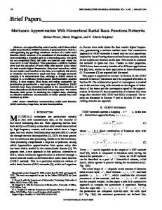
To test the stability and the convergence properties of the new RBF approximation algorithm, we consider a one dimensional double well system, with drift function fθ (t, Xt ) = 4Xt (θ − Xt2 ), θ > 0, and constant diffusion. This is a non-linear dynamical system, whose stationary distribution has two stable states Xt = ±θ. The system is driven by white noise and according to the strength of the random fluctuation (system noise coefficient Σ) occasionally flips from one stable state to the other (Figure 1(a)). In the simulations we consider a time window of ten units (t0 = 0, tf = 10). The true parameters, that generated the sample path, are Σtrue = 0.8 and θtrue = 1.0. The observation density was fixed to two per time unit (i.e. twenty observations in total). To provide robust results one hundred different realisations of the observation noise were used. The basis functions were Gaussian (7) with centres ci chosen equal spaced within the time window and widths λi sufficiently large to permit overlap of neighbouring basis functions. In Figure 1(b), we compare the results obtained from the RBF approximation algorithm, with basis function density M = 40, per time unit, (Mtot = 800) against the true posterior obtained from a Hybrid Monte Carlo (HMC) method. We note that although the variance of the RBF approximation is slightly underestimated, the mean path matches the true HMC results quite well, as was the case in VGPA. The new RBF approximation algorithm is extremely stable and 1.5
2
1
1.5 1
0
0.5
X(t)
X(t)
0.5
−0.5
0
−1
−0.5
−1.5 −2 0
−1
1
2
3
4
5 t
6
7
8
9
−1.5 0
10
1
2
3
4
5
6
7
8
9
10
t
(a) True sample path
(b) HMC vs RBF approximation
Fig. 1: (a) Sample path of a double well potential system used in the experiments. In (b) we compare the approximated marginal mean and variances (of a single realisation) between the “true” HMC estimates (solid lines) and the RBF variational algorithm (dashed lines) solutions. The crosses indicate the noisy observations.
converges to the original VGPA, given a sufficient number of basis functions. Figure 2(a) shows convergence of the free energy of the RBF approximation to the VGPA results after thirty five basis functions per time unit (Mtot = 700) and this is also apparent in comparing the “correct” KL(p,q) divergence [4], between the approximations q and the posterior p derived from the HMC, Figure 2(b). The computational time for the RBF method is similar or slightly higher, however it is more robust and stable in practice. The VGPA approximation can also be used to compute marginal likelihood based estimates of (hyper-)parameters
500
ESANN'2009 proceedings, European Symposium on Artificial Neural Networks - Advances in Computational Intelligence and Learning. Bruges (Belgium), 22-24 April 2009, d-side publi., ISBN 2-930307-09-9.
21
50
20 45
40
18 KL
F(M | θ, Σ, R)
19
17
35
16 30 15 14 0
20
40
60
80
25 0
100
20
40
M
60
80
100
M
(a) Free energy
(b) KL divergence
Fig. 2: (a) Comparison of the free energy, at convergence, between the RBF algorithm (squares, dashed lines) and the original VGPA (solid line, shaded area). The plot shows the 25, 50 and 75 percentiles (from 100 realisations) of the free energy as a function of basis function density. (b) shows a similar plot (for one realisation) for the integral of the KL(p,q), between the “true” (HMC) and approximate VGPA (dashed line, shaded area) and RBF (squares, dashed lines) posteriors, over the whole time window [t0 − tf ]. including the system noise and the drift parameters [9]. In the RBF version this is also possible and empirical results show that this is faster and more robust compared to VGPA. As shown in profile marginal likelihood plots in Figures 3(a) and 3(b), even with a relative small basis function density, the Σ and θ minima are very close to the ones determined by the VGPA. For the Σ we need around thirty basis functions (M = 30), to reach the same minimum, whereas for the θ parameter the minimum is almost identical using only ten basis functions (M = 10), per time unit. These conclusions are supported by further experiments on 100 realisations (not shown in the present paper), which show consistency in the estimates of the maximum marginal likelihood parameters both in value and variability. 26
24 M = 10 M = 20 M = 30 VGPA
24
22
M = 10 M = 20 M = 30 VGPA
22 F(θ | Σ)
F(Σ | θ)
20 20 18
18
16 16 14
14 12 0.2
0.3
0.4
0.5
0.6
0.7 Σtest
0.8
0.9
1
1.1
12 0.5
1.2
(a) Σ profile
0.6
0.7
0.8
0.9
1 Θtest
1.1
1.2
1.3
1.4
1.5
(b) θ profile
Fig. 3: (a) Profile marginal likelihood for the system noise coefficient Σ keeping the drift parameter θ fixed to the true one. (b) as (a) but for the drift parameter θ keeping Σ fixed to its true value. Both simulations run for M = 10, M = 20 and M = 30 and compared with the profiles from the VGPA on a typical realisation of the observations.
501
ESANN'2009 proceedings, European Symposium on Artificial Neural Networks - Advances in Computational Intelligence and Learning. Bruges (Belgium), 22-24 April 2009, d-side publi., ISBN 2-930307-09-9.
5
Conclusions
We have presented a new variational radial basis function approximation for inference for diffusion processes. Results show that the new algorithm converges to the original VGPA with a relatively small number of basis functions per time unit, needing only 40% of the number of parameters required in the VGPA. We expect that further work on the choice of the basis functions will further reduce this. Thus far only Gaussian basis functions have been considered, with fixed centres and widths. A future approach should include different basis functions that will better capture the roughness of the variational (control) parameters of the original algorithm, along with an adaptive (re)estimation scheme for the widths of the basis functions. We go on to show estimation of (hyper-)parameters within the SDE is remarkably stable to the number of basis functions used in the RBF. Reducing the number of parameters makes it possible to apply the RBF approximation to larger time windows, although this is limited by the underlying discrete computational framework. We are investigating the possibility of computing entirely in continuous time using the basis function expansion. Acknowledgements The authors acknowledge the help of Prof. Manfred Opper, whose useful comments help to better shape the theoretical part of the RBF approximations.
References [1] Peter E. Kloeden and Eckhard Platen. Numerical Solutions of Stochastic Differential Equations, Springer-Verlag, Berlin, 1992. [2] Christopher M. Bishop. Neural Networks for Pattern Recognition, Oxford University Press, New York, 1995. [3] D. S. Broomhead and D. Lowe. Multivariate functional interpolation and adaptive networks. Complex Systems, 2:321-355, 1988. [4] S. Kullback and R. A. Leibler, On information and sufficiency. Annal of Mathematical Statistics, 22:79-86, 1951. [5] A. Golightly and D. J. Wilkinson. Bayesian inference for non-linear multivariate diffusion models observed with error. Computational Statistics and Data Analysis, 2007. Accepted. [6] C. Archambeau, D. Cornford, M. Opper and J. Shawe Taylor. Gaussian process approximation of stochastic differential equations. Journal of Machine Learning Research, Workshop and Conference Proceedings, 1:1-16, 2007. [7] V. K˚ urkova and K. Hlavaˇckova. Approximation of Continuous Functions by RBF and KBF Networks. ESANN, Proceedings, pp. 167-74, 1994. [8] T. Jaakkola. Tutorial on variational approximation methods. In M. Opper and D. Saad, editors, Advanced Mean Field Methods: Theory and Practise, The MIT press, 2001. [9] C. Archambeau, M. Opper, Y. Shen, D. Cornford, J. Shawe-Taylor. Variational Inference for Diffusion Processes. In C. Platt, D. Koller, Y. Singer and S. Roweis editors, Neural Information Processing Systems (NIPS) 20, pages 17-24, 2008. The MIT Press. [10] M. D. Vrettas, Y. Shen and D. Cornford. Derivations of Variational Gaussian Process Approximation. Technical Report (NCRG/2008/002). Neural Computing Research Group, Aston University, Birmingham, B4 7ET, United Kingdom, March 2008.
502