synchronization overheads involved in the solution process. The methodology presented here is based on the matrix inverse factors (W-matrix) approach to the ...
1023
Transactions on Power Systems, Vol. 7. No. 3, August 1992
A W-MATRIX METHODOLOGY FOR SOLVING SPARSE NETWORK EQUATIONS ON MULTIPROCESSOR COMPUTERS
A. Padilha UNESP-Ilha
Solteira-Brazil
Abstract: This paper describes a methodology for solving efficiently the sparse network equations on multiprocessor computers. The methodology is based on the matrix inverse factors (W-matrix) approach to the direct solution phase of Az = b systems. A partitioning scheme of W-matrix , based on the leaf-nodes of the factorization path tree, is proposed. The methodology allows the performance of all the updating operations on vector b in parallel, within each partition, using a row-oriented processing. The approach takes advantage of the processing power of the individual processors. Performance results are presented and discussed. Keywords: Power Flow, Stability, Parallel Processing, Sparsity, Direct Solutions.
INTRODUCTION It is a matter of fact that low-cost multiprocessor computers are now available featuring supercomputer-like performances. For instance, new powerful multiprocessor machines have been announced which can offer peak performance ranging from 480 to 7600 Mflops with 8-128 processors interconnected using a message passing architecture [l] or ranging from 2 to 130 Gflops, up to about 65,000 processors, using a shared memory architecture [2]. Even though peak performance is not straightforward to achieve because it depends on how the parallel algorithms are mapped to the parallel architectures, there is no doubt that the power industry may be one of the first to take advantage of this computer technology. Many power systems problems require the repetitive solution of a large set of sparse linear equations and this task represents the most time consuming part of the overall solution. For this reason, the effort for solving efficiently the linear network equations on multiprocessor hardware is one of most promising ways to take advantage of parallel processing in power systems applications. It has been recognized that the parallel solution of sparse network equations is not a smooth task, because the great number of precedence relations among arithmetic operations leads the solution processing to have a large amount of idle time [3,4]. If one processor has assigned very simple tasks, a multiplication for example, the precedent relationship web will make the communication and/or synchronization over-
91 SM 482-0 PWRS A paper recomended and approved by the IEEE Power System Engineering Committee of the IEEE Power Engineering Society for presentation at the IEEE/PES 1991 Summer Meeting, San Diego, California July 20 - August 1, 1991. Manuscript submitted January 30, 1991; made available for printing Hay 17, 1991.
A. Morelato UNICAMP- CampinasBrazil
heads increase a lot and so offset the advantages of parallel processing. This paper describes' a methodology for decomposing the repeat solution process of the equation Az = b into independent tasks to be done in parallel. The approach allows the task unit to be assigned to each processor to be somewhat more coarse-grained than elemental arithmetic operations. Therefore, it is possible to take advantage of the powerful processors that constitutes a multiprocessor environment and, at the same time, to reduce the amount of communication and synchronization overheads involved in the solution process. The methodology presented here is based on the matrix inverse factors (W-matrix) approach to the direct solution phase of Ax = b systems, as proposed in [5]. The W-matrix approach does not Seem to be advantageous for processing of the repeat solution on conventional serial machines, as shown in the discussion of [SI. On the other hand, it seems very promising for parallel processing methods, considering its properties of decoupling the elementary operations.
Problem Formulation A set of linear network equations is usually expressed as:
Ax = b
(1)
where A is a nonsingular matrix of order n , the vector z is the unknown solution and b is the given independent vector, which will be considered a full vector. The matrix A is assumed to be sparse and symmetric. The standard solution method for (1) comprises a sparsityoriented LDU decomposition of A followed by forward, diagonal and backward operations on the vector b:
A
= LDU
(2)
where L and U = L' are lower and upper triangular matrices with unity elements in the diagonals and D is a diagonal matrix. The L-matrix can be expanded as L = L1 LZ ...L, such that each Li is an identity matrix except for the ith column, which contains the column i of L. The computation of L and U is preceded by ordering of rows and columns of the matrix, usually to minimize the number of nonzero elements. The solution process described by equation (3) may be seen as an ordered sequence of updating operations applied to the right hand side vector. In this paper the problem to be tackled is how to perform efficiently the solution (3) on a multipre cessor environment in such a manner to take advantage of its
0885-89501p2so3.00 Q 1992 IEEE
I
1024
potential computing speedup and so to realize the solution in the least time. More specifically, the challenges are: how to decompose the repeat solution process into independent tasks which have an appropriate size, and how to schedule the tasks on the processors in such a way as to reduce the communication and synchronization overheads, achieving a minimum solution time.
BASIS OF THE METHODOLOGY In this section the foundations on which the proposed approach is based will be presented briefly. The 20-node system [7], whose network is shown in Figure 1, will be taken as a tutorial example with no loss of generality.
2 shows the path tree of the example network obtained from the L-matrix structure using the ML-MD ordering scheme [8]. Using the MD-MNP scheme [9], the path tree for the example network is, by chance, exactly the same as the classical MD scheme. A node of the factorization path tree is to be said a leaf if it has no predecessor. The depth (or level) of a node can be defined as the maximum number of nodes in the tree which precede it. Both concepts can be associated and so it can be said that a leaf of depth i is a leaf provided that all the nodes of depth i-1 have been reduced. For example, in the path tree illustrated in Figure 2 the nodes { 1,2,3,4,5,6,7,8} are leaves of depth 0 and the nodes {9,11,14,15,16} are leaves of depth 1. Table A.1 in Appendix A shows the number of leaves at the different depths obtained from two test networks and using several ordering criteria. The performance of the methodology presented in the paper is not significantly affected by the ordering schemes, though some schemes can be more friendly than others. The ML-MD scheme provides an ordered sequence of nodes that matches automatically the leaves of successive depths. Otherwise, the MD-MNP scheme requires extra work after ordering to rearrange the nodes.
Partitioning Scheme Assuming that the LDU decomposition has been carried out in an appropriate way, the goal is to perform in parallel the operations on vector b described by equation (3). This equation can be transformed and expanded according to the idea of reference [5] as:
z = W ' D - ' W b = W:Wj ...WAD"Wn 3
12
Figure 1: The 20-node example network Factorization Paths and Ordering Schemes
As is well known, the precedence relations among operations on columns and rows to perform the LDU decomposition and forward/backward solutions can be depicted by the factorization path graph [7]. It is also known that different ordering schemes can change the shape of the path tree and alter the number of fill-in elements of L and L-I. Figure
1
4
7
6
5
8
...W2Wib
(4)
2
11
3
depth
1
3
where Wi = Ly', a = 1 , . .. ,n . The adjacent matrices Wi can be combined in different ways giving rise to different partitions of matrix W . The advantage of this approach is that all multiplications between inverse factors and components of vector b within each partition become independent and can be performed in parallel. Unfortunately, the necessary additions to update each component of b cannot all be performed simultaneously. On the other hand, the partitions may be utilized to keep under control the additional fills that can be created in the W-matrix. Reference [5] proposes to perform the direct solution phase by breaking it up into partitions whose number depends on the number of additional fill-in elements allowed within each partition. This partitioning technique has been enhanced in reference [SI. The partitioning scheme proposed in this paper consists of breaking the W-matrix according the depths of the factorization path tree, as follows: 0
each partition p is assigned to a depth of the path tree, i. e. all the nodes which are leaves of depth p belong to the partition;
0
the assignment proceeds until some previously chosen depth (called break-in depth) is achieved and then all the remaining nodes of the tree are gathered into one partition (called last partition).
4 5 018
6
6 20
7
Figure 2: Path tree after ML-MD ordering
The choice of the break-in depth is heuristic but not critical for the solving methodology because the number of leaves
I
1025
'
by depth decreases quickly at the top but slowly after a few depths, as shown in Table A.1 in the Appendix A. A simple heuristic rule relating the number of nodes in the last partition with the number of available processors may be used, for example. Figure 3 shows the W-matrix structure from the 20-node example after the application of the partitioning scheme proposed, assuming the path tree ML-MD illustrated in Figure 2 and taking the break-in depth as 2. Note that the matrix is divided into three partitions composed of nodes {1,2,3,4,5,6,7,8}, {9,11,14,15,16} and { 10,12,13,17,18,19,20} respectively. Furthermore, note the one additional fill-in element in the last partition whereas there are no additional fills in the two first partitions, as would be expected.
1 2 3 4
5 6
7 8 9
X
I(
11
X
X
14
X
15
X
16
X
X
10
X
X
X
12
X
X
X
19
X
X
%
x original element
X
X O
X X
x x x
8
X
18
X
8 8
8
X
17
8
x
X
13 K
20
X
X
8 8 fill-in element
X
@
@
@
8
X
8 8 8 8 8 X x . 8 8 8 8 8 r
w
fill-in element
Figure 3: Partitioning of W-matrix In this scheme, all the information needed to generate the partitions can be obtained straightforwardly from the network factorization path tree. The partitioning algorithm is simple and easy to implement. The elements of Wi matrices, except the last partition, can be obtained directly from L-matrix elements, not requiring extra work. The proposed scheme guarantees that additional fills will be created only in the last partition. As a matter of fact, if a partition does not have any two nodes which are predecessors of each other, then no additional fills are produced in the partition matrix. This condition can be easily validated remembering what is occurring with the network when the factorization proceeds, node by node, according to the path tree. It should be noted that the condition is sufficient but not necessary. If two nodes of different depths are put together into the same partition, it is not assured that additional fills will be yielded because it may happen that the place has been already filled. This is the case of the element (13,lO) in Figure 3. Reference [lo] presents a partitioning technique based on the levels of the factorization path graph but the difference is
twofold: the goal to be achieved and the criterion to create a partition. In reference [lo] the objective of partitioning is to generate the minimum number of extra fill-in, aiming to minimize the number of elementary arithmetic operations to be performed on a vector computer. Otherwise, our partitioning scheme aims at generating the minimal number of partitions with the maximum number of independent tasks to be assigned to processors on a multiprocessor computer. The idea behind our proposed scheme is to take advantage of the great number of leaf-nodes in the first partitions because they correspond to independent tasks. When the leaf-nodes begin to fade, because the precedence relationships become stronger, then all the remaining nodes are gathered disregarding the extra fills. This action gives rise to new independent tasks in the last partition but the price to be paid is to perform the extra fills. The last partition concentrates all the additional fills, but it can be shown that those extra fills do not delay the parallel processing of the partition, considering that the lowest row of the partition is always full. Indeed, the number of nonzero elements of the lowest row of the L-' matrix corresponds to the number of nodes which precede the ultimate node in the factorization path tree. Therefore, the time spent to process the lowest row determines the least time to process the last partition. It is possible to use partitioning schemes that combine nodes from more than one level in a given partition with no extra fills, as shown in [6] and [lo]. Particularly, [lo] describes a simple but very effective way to find out the proper nodes, although it was valid only for MD ordering. Those procedures can slightly rearrange the nodes belonging to the first partitions but it is not clear that this leads to smallest solution time in general.
Formation of the W-matrices The computation of the W-matrices elements is straightforward for the first ( p - 1) partitions because they are equal to the off-diagonal elements of L-matrix with the sign reversed. This is valid providing that all nodes within each partition are at the same level in the factorization tree. The computation of the last partition elements requires some extra work. They might be directly obtained from the multiplication of the adjacent matrices W,corresponding to the last partition. The effort is reasonable remembering that a matrix W,is an identity matrix except for the Cth column. This is the approach used in the paper. Otherwise, the computation of the Wmatrix for the last partition can be done in parallel utilizing, e.g. the technique proposed in [Ill. However, the construction of the W-matrices is one step that must be performed only once in the repeat solution process and it may not be worth doing it in parallel. It has been recognized that parallelism is best used for steps that require a significant number of cycles.
TASK SCHEDULING This section deals with the decomposition of the repeat solution process into independent tasks, i. e. the amount of work which can be done at the same time, in any order, and without communicating with another task. Also is discussed what is the best size of the task to be assigned to each processor on multiprocessor environments. Moreover, the task
I 1026
scheduling strategy for distributing the tasks among the processors is addressed.
IndeDendent Tasks The repeat solution comprises essentially an ordered sequence of updating tasks operating on the components of the vector b, where each one is formed by arithmetic operations of multiplication and addition. It is possible to assign each one of these elementary arithmetic operations to a processor in order to exploit the maximum amount of parallelism. However, it is not clear that the solution with the maximum parallelism is always the fastest. The communication or synchronization overheads may increase a lot producing significant delays. Unfortunately, this is the case of the repeat solution process due to the large number of precedence relations among the operations, i. e. the elementary operations are not independent of each other. The application of the W-matrix approach to the repeat solution allows all multiplications between inverse factors and elements of b to be independent each other - within each partition - and could be carried out in parallel. However, the additions cannot all be performed at the same time. This fact does not mean that there is no parallelism even in the additions but that some of them cannot be performed simultaneously because each one has to take the most updated value of b, which is under processing at the same time. In other words, some additions (not previously known) are not independent and to find out its precedent relationships is time consuming. It should be noted that the degree of dependence of the u p dating tasks depends upon whether the solution is performed by columns or by rows. To illustrate this point take the 20node example system and suppose the forward solution is to be performed by columns (conventional forward). The operations on vector b corresponding to partition 1 are: task number
arithmetic operations
The idea presented here is to gather b y row8 the operations to be performed. In doing this, a l l the updating tasks within each partition become completely independent of each other. For the example system, the operations on vector b, referring to partition 1, can be grouped as:
task number
arithmetic operations
Note that there are no conflicts here because each compe nent of b is updated only once within the partition. Therefore, the chunk of updating tasks corresponding to a row of each partition is independent and can be done in parallel. However, the forward and backward processing by rows requires double sets of tables for indices of rows and columns of the lower and upper triangular W-matrices.
s ~ h e d u i n gStrategy The strategy proposed here is to schedule on each processor the operations corresponding to a row of each partition. It should be kept in mind that multiprocessor environments are equipped with powerful unit processors and then it seems a sound strategy to perform the mult-add elementary operations inside the hardware in order t o exploit its computing efficiency. This strategy seeks to match the parallel algorithm to the parallel architecture. The precedent relations that give rise to delays - are replaced by mult-add operations performed inside the processor node without external communication. Parallelism within a row could be exploited if the processor node is provided with binary adder facilities. The scheduling strategy should take into account the number of available processors. A simple but efficient strategy consists of assigning several rows to one processor using a wrap mapping style, ? that processor zero gets row 1, nproc+l, 2nproc+l, , where nproc is the number of available processors. This is the strategy used in taking the results presented further. It is evident that if the number of processors is greater than the number of rows to be performed in a partition, then the maximum load of one processor corresponds to just one row. It should be noted that the size of the row-oriented tasks is not uniform because the number of elements per row is not the same, ranging from 1 to 10 for the networks simulated. Load unbalancing is not an issue if the goal is the solution in minimum time. The solution time spent to solve a partition is always given by the processor which has assigned the row with the greatest number of elements. It is does not matter if some processors remain idle for a while because they cannot speedup the solution. The solution with the best load balance is not necessarily the fastest. The goal is not to keep
-
...
where w,,, is the element ( i , j ) of partition 1. It can be seen that the additions to update 813, as indicated in tasks #2 and #9, cannot be processed simultaneously to assure correct results and so they are not independent. The same kind of conflict can be found in the rows 15, 18 and 20. In the backward solution there is no problem because the conventional backward is usually performed by rows.
I
1027
busy all the processors but using the available processors in such a way to achieve the fastest solution.
THE LAST PARTITION Taking into account that the direct solution will be performed by rows, it becomes advantageous to handle the last partition as an unique one. According to the partitioning scheme equation (4) can be expressed as:
where the diagonal operations D-' were split into D;:', concerning the early (p - 1) partitions, and DG1 , concerning the last partition. As the operations corresponding to the last partition are not affected by the operations D;:,, equation ( 5 ) is equivalent to:
parallelism achieved by the presented approach is adequate to minimize the influence of hardware overheads in both architectures. The performance of the methodology can be evaluated considering the simulation results depicted in Table I and Table I1 showing the maximum number of mult-add operations corresponding to eachsserial step of the solution for several numbers of partitions (not counting the operations with diagonal elements). The ML-MD ordering was used. In Table I (JEEG 118 system) it can be seen that the first serial step requires at most 4 mult-add operations, i. e. the greatest number of nonzero elements in one row of the partition is 4. If it is assumed, for simplicity, that the number of processors available is large enough, then the total solution time (including the idle time) to process this step is the time spent to do 4 multiplications and 4 additions. The last partition step is the bottleneck because the lowest row of Wip is always full. The impact of the last partition could be reduced if the number of partitions is increased, however the increase in the backward operations may offset this gain and increase the total solution time. The number in parentheses denotes the additional fills Table I 2
n the forward, diagonal and where WiP = W ~ D ~ ' Wrepresents backward aggregated operations on the last partition. In the last partition, the forward, diagonal and backward solutions may be gathered, and so all the operations can be expressed as the product of matrix W[, by the updated components of vector b. The result is that the tasks of updating the last partition elements of b become independent if they were performed by rows, as the other partitions are. Moreover, the total number of operations is smaller than in the conventional procedure and the number of serial steps is reduced. Though Wip is a full matrix, its additional fills do not increase the solution time of the last partition because it depends essentially on the number of nonzero elements in the lowest row (it is always full) and the number of processors available. On the contrary, the solution time decreases because the serial steps of forward, diagonal and backward solutions will be performed a t the same time as the forward step.
PERFORMANCE RESULTS
1
-
118 node system. 3
Partitions4 (151) 4 4 4 -
I
69
I
49
I
-
22 -
14
-
6 6 3 3 47
6 3 3 46
- I-
6
7
4 4 3 2 10 9 6 6 3 3 54
(0) 4 4 4 3 2 2
8 8 9 6 6 3 3 62
Partitions 7 9 6 8
3858: 1886) (981)
(570)
9 7 5 4 4 4 -
9
9
7
7
5 4 4 4 4 -
15 10 10 9
5 4 4 4 4 3 46 17 15 10 10 9
7 7
7 7
6
6 167 -
9
7
The methodology proposed here can be used either on a message-passing or shared-memory architecture, even though the characteristics of the approach are best fitted to sharedmemory or hybrid machines (each processor accesses local memory too). In this case, the vector b is stored in the shared memory which can be accessed for every processor through global variables. The access time is the same as the local memory references, neglecting common bus contention. Therefore, the processors are able to update the vector b, within each partition, without communication overhead. Before carrying out the next partition, all the processors involved must overcome one synchronization barrier. As for messagepassing machines, the need of broadcasting the updated values of vector b among the processors, before carrying out the next partition, introduces a communication overhead which is inherent to this architecture. Anyway, the coarse-grained
4 4 3
-
-
total
5
(7) 0 4 4
5 4 4 -
97 -
72
-
10 10 9
10 9
7 7
-
7 7 6 154
6 165
56 -
157
I 1028
produced in the lower triangular matrix of the last partition. Note that the no-fills condition, attained with 7 partitions, does not produce the speedest solution time. In summary, Table I shows that the direct solution calculations for the IEEE118 network can be performed in the time equivalent bo 46 floating point operations of multiplication and addition if the number of processors is large enough (62 processors in this case). By comparison, if the partitioning scheme of [lo] was used, no extra fills would be created but the solution time would be equivalent to 68 flops (12 partitions), considering the IEEE118 network. For a 1729-node system, Table I1 shows that using 7 partitions the calculations correspond to only 154 floating point mult-add operations. Figure 4 illustrates how the number of processors can affect the fastest solution time for different network sizes. The gain is given by G = t s / t p , where t s is the total mult-adds operations for the serial solution (using MD ordering), and tp is the number of operation8 obtained for the parallel solution (using ML-MD ordering). The maximum usable number denotes the number of processor that must be available to get the least solution time. It is given by the greater of two numbers: the number of rows of the first partitions with nonzero elements (forward) or the number of leaf-nodes of the path tree (backward). The maximum usable number is 62, 161, 402 and 956 processors for the simulated networks, respectively. This kind of graphics allows finding the least solution time possible to achieve if the number of available processors is previously fixed. The methodology was implemented in a multiprocessor computer and the performance results are presented in A p pendix B. GJ 50
.
40
.
more and more offered by the processor unit hardware. The performance results show that the potential speedup of the solution time is essentially bounded by the floating point operation capability of each processor, denoting that the methodology is a suitable way to exploit the growing power of the computing technology.
REFERENCES [l] “Intel builds new supercomputer around I860”, Computer, pp.101, March 1990. [2] Rettberg R.D., Crowther W.R.,Carvey P.P. & Tomlinson R.S.,“The Monarch Parallel Processor Hardware Design”, Computer, pp.18-28, April 1990.
[3] Braach Jr. F.M., Van Ness J.E. & Kang S.C.,“Simulation of a Multiprocessor Network for Power System Problems”, IEEE Transactions on PAS, vol. PAS-101, n. 2, pp. 295-301, February 1982. [4] Van Ness J.E., discussion in reference [5].
[a] Enns M.K., Tinney W.F. & Alvarado F.L., “Sparse M k trix Inverse Factors”, IEEE Transactions on Power Systems, vol. 5, n. 2, pp. 466473, May 1990.
[SI Alvarado F.L., Yu D.C. & Betancourt R., “Partitioned Sparse A-’ Methods”, IEEE Transactions on Power Systems, vol. 5, n. 2, pp. 452-459, May 1990.
S.M.,“Sparse Vector Methods”, IEEE Trans. on PAS, vol. 104,n. 2, pp.295-301, February 1985.
[7] Tinney W.F., Brandwajn V. & Chan
[SI Betancourt R., “An Efficient Heuristic Ordering Algo-
16 processors ID 64 processors 0 max. usable number
rithm for Partial Matrix Refactorization”, IEEE llans. on Power Systems, vol. 3, n. 3, pp 1181-1187, August 1988.
[Q] Gomes A. & Franquelo L.G.,“An Efficient Ordering Algorithm to Improve Sparse Vector Methods”, IEEE ’Rans. on Power Systems, vol. 3, n. 4,pp. 1538-1544, November 1988.
30 .
[IO] Gomes A. & Betancourt R.,“Implementation of the Fast 20
10
Decoupled Load Flow on a Vector Computer”, IEEE llans. on Power Systems, vol. 5, n. 3, pp. 977-983, August 1990.
. ’
0-
118
320
72
-
system
Figure 4: Gain versus system size.
1
(111 Betancourt R. & Alvarado F.,” Parallel Inversion of Sparse Matrices”, IEEE Transactions on Power Systems”, vol. 1, n. 1, ppI 74-81, February 1986.
Biographies
CONCLUSIONS
Antonio Padilha Feltrin was born in Meridiano, Brazil in 1956. He received the B.Sc. degree in 1980 from EFEI and the M.Sc. degree in 1986 from Unicamp. Since 1981 he has been an Assistant Professor at UnespIlha Solteira. He is currently a candidate to Ph.D. degree at Unicamp.
A methodology has been described for solving sparse network linear equations on a multiprocessor computer using a partitioned W-matrix approach to the direct solution phase. The methodology allows all the rows of each partition to be processed in parallel and leads to a task scheduling strategy fitted to multiprocessor computer architectures. The a p proach takes full advantage of the powerful megaflops features
Andre L. Morelato F’ransa received the B.Sc. degree in 1970 from ITA and the Ph.D. degree in 1982 from Unicamp, Brazil, where he is currently an Associate Professor of Electrical Engineering. His general research interests are in the area of control and stability of electrical power systems and distribution automation.
1029
APPENDIX h
APPENDIX B
Table A.1- Distribution of leaves at different depths for several orderings and systems.
The methodology described in the paper was implemented in a multiprocessor computer (Parallel Preferential Processor - P3) under developing by the Federal Telecommunications R&D Center (CPqD) in Brazil. The version we are using consists of eight iAPX 2861287 based boards, connected in a common-bus 10 Mbytes/s bandwidth architecture. The common-bus uses a daisy-chain scheme for controlling the concurrent accesses. Each board contains a local memory of 512K bytes RAM and can access 2048K bytes of shared memory. Each CPU board is loaded with DOS operating system, extended with concurrent processing facilities. The tests were carried out by solving a I=YV system, where Y is the complex nodal admittance matrix, I is the current injection vector and V is the voltage vector. All variables are stored in the local memories except vector V which is only stored in the shared memory. This data structure takes advantage of the machine architecture allowing the bus contention to be minimized. Figure B . l compares the gain obtained using P3 with theoretical gains, regarding 50 repeated solutions of equation I=YV for the four networks. The theoretical gain here mentioned is slightly different from the gains shown in Figure 4, for the operations with the diagonal elements are now included whereas they were neglected before. G4
U
The number in square brackets denotes the original offdiagonal nonzero elements in L-matrix. The number in parentheses denotes the fill-in elements.
I P 3
118
320
725
1729 sy’st.
Figure B.l: Experimental results using eight processors
The experimental results were obtained using eight processors, the ordering scheme was MLMD and the last partition was handled as one block. The number of partitions used are 7,8,11 and 12, respectively. The codes were written in Fortran 77, extended with library functions to support parallelism. The results show that the measured gains are very close to the theoretical ones, indicating that the communication overhead and common-bus contention are not significant.
1030
Discussion
Fernando L. Alvarado (The University of Wisconsin, Madison, Wisconsin): This paper is very much on target: Partitioned Inverse Methods represent a major new technology for parallel computation. This paper makes one important contribution to this new technology: the handling of the "last partition." Explicit inversion of the last partition is desirable because it reduces the number of parallel steps at no significant cost in terms of number of added fills. More important, however, is that this enables the ready use of vectorization methods in the handling of the last partition. Recent experiments in sparse matrices have indicated that the gains from parallelism in the first levels of the tree are limited unless something is done to handle the last block, which is precisely the main contribution of this paper. The paper, regretably, contains a misleading statement: The computation of the W-matrices is straightforward for the first ( p - I ) partitions because they are equal to the off-diagonal elements of (the) L-matrix with the sign reversed. This is valid provid(ed) that all nodes within each partition are at the same level in the factorization tree. In the partitioned inverse method it is not necessary
for all elements in a partition to come from the same level in the factorization tree. Doing so unnecessarily increases the number of partitions. The computational expense in computing mutiple-level partitions is usually small, and is needed only once, not every solution step. The authors can claim that the gains of aggregating multiple levels into a single partition are comparatively small. What is at stake here, however, is that this statement can create a misunderstanding of the nature of the partitioned inverse process. Moreover, as vectorization improves the * handling of the last partition, the improvement attained by, reducing the number of partitions becomcs once again significant.
correspondent element of the L-matrix with the sign reversed. None additional computation is required for those partitions but however the computation of the elements of the last partition requires some extra work. This fact can be understood as follows. The matrix W can be obtained performing sequentially, from right to left, the following operdons: t t t -1 W = W 1 W 2 ... W n D Wn ... W2W1 where Wi=%-l is an identity matrix (nxn) except for the i-th column in which $he off-diaeonal elements are eaual to the comspondent
-i-
=vema-l Let us consider the property below. Propertv : Let j and k two nodes of a factorization tree with n nodes ordered according to the depth of the tree. If the nodes J and k belong to the same level of the factorization tree then wk.wj = w k + wj - In
where In denotes an identity matrix (nxn). Let us consider, without loss of generality, that the nodes j and k are at the level zero. Therefore, the general shape of the matrices w j and Wk is: nr nO nO N nO
N
Manuscript received August 9, 1991.
A. PADILHA , A. MORELATO : We would like to thank Dr. Alvarado for his interest in this paper and for the valuable comments. The discussion is welcomed because allows the authors to clear up some points in the paper that were briefly mentioned due to the lack of space. The partitioned inverse method consists of an ordered sequence of matricial operations on the independent vector. The operations can be described by matrices Wi = L i l , i=1,2,...,n , where n is the number of network nodes ( and columns of the L-matrix). Each matrix Wi is an identity matrix except for the i-th column. Each partition of the matrix W corresponds to grouping some adjacent matrices Wb Even though the inverse method allows several other partitioning approaches, we propose to combine the matrices Wi that belong to the same level of the network factorization tree except the last ones which are handled as a block. In doing so we are exploiting the great deal of parallelism that is found at the first levels of the tree. Moreover, all the additional fills come up in the last partition only, where they cannot stretch the solution time. In our partitioning scheme the number of partitions is an independent variable which can be chosen aiming to minimize the solution time. For example, the Table I of the paper shows that is better to use four partitions for the 118-network. A very simple algorithm, taking into account the factorization tree and the number of available processors, can be used as part of the partitioning scheme to estimate the convenient figure A by-product of this partitioning scheme is that the computation of the inverse factors corresponding to all the partitions but the last one is quite simple. Indeed, each inverse factor is equal to the
4
4
nonzero elements in the j-th column
nonzero elements in the k-th column
where no is the number of nodes with level 0 and nr is the number of remaining nodes. Note that the matrices can be seen as decomposed into four submauices: two block diagonal identity matrices (which are essential to see how the property works), one upper right null mamx and one lower left matrix which contains the nonzero elements ofG-1. It is easy to see that the product WkWj has exactly the same shape of the matrices Wj or w k and, moreover , its nonzero elements correspond to the j-th column of Wj superimposed to the k-th column of W k None original element is modified. nO nr
I
1
Wk.Wj =
j k The property can be successively applied to the nodes of each at different levels. partition except for the last one whose nodes Manuscript received November 8, 1991.