A Methodology for Solving the Equations Arising in Nonlinear ...

To the Graduate Council: I am submitting herewith a dissertation written by Kaiyu Wang entitled “A Methodology for Solving the Equations Arising in Nonlinear Parameter Identification Problems: Application to Induction Machines". I have examined the final electronic copy of this dissertation for form and content and recommend that it be accepted in partial fulfillment of the requirements for the degree of Doctor of Philosophy, with a major in Electrical Engineering. John Chiasson Major Professor We have read this dissertation and recommend its acceptance: Leon Tolbert J. Douglas Birdwell Tim Schulze

Accepted for the Council: Anne Mayhew Vice Chancellor and Dean of Graduate Studies

(Original signatures are on file with official student records.)

A Methodology for Solving the Equations Arising in Nonlinear Parameter Identification Problems: Application to Induction Machines

A Dissertation Presented for the Doctor of Philosophy Degree The University of Tennessee, Knoxville Kaiyu Wang December 2005

Copyright  2005 by Kaiyu Wang. All rights reserved.

ii

Dedication This dissertation is dedicated to my wife Mei. Thanks for all the love and great patience throughout the years. It is also dedicated to my parents, who have supported and encouraged me to persevere through life’s challenges.

iii

Acknowledgements First and foremost, I would like to express my deepest appreciation to my major advisor, Dr. John Chiasson, for his support, all of his help and instructions during my study and research. Also, I would like to thank Dr. Leon Tolbert, for his great help and kind support during my study at UTK. Many thanks to Dr. Birdwell and Dr. Schulze for their serving on my thesis committee, reading this thesis and providing invaluable suggestions and constructive comments. In addition, I would like to thank the other faculty, staff and students in the Power Electronics laboratory: Mengwei Li, Weston Johnson, Surin Khomfoi, Yan Xu, Hui Zhang, Wendy, Lucy, … who create a friendly working environment.

iv

Abstract This dissertation presents a method that can be used to identify the parameters of a class of systems whose regressor models are nonlinear in the parameters. The technique is based on classical elimination theory, and it guarantees that the solution for the parameters which minimize a least-squares criterion can be found in a finite number of steps. The proposed methodology begins with an input-output linear overparameterized model whose parameters are rationally related.

After

making

appropriate

substitutions

that

account

for

the

overparameterization, the problem is transformed into a nonlinear least-squares problem that is not overparameterized. The extrema equations are computed, and a nonlinear transformation is carried out to convert them to polynomial equations in the unknown parameters. It is then show how these polynomial equations can be solved using elimination theory using resultants. The optimization problem reduces to a numerical computation of the roots of a polynomial in a single variable. This nonlinear least-squares method is applied to the identification of the parameters of an induction motor. A major difficulty with the induction motor is that the rotor’s state variables are not available measurements so that the system identification model cannot be made linear in the parameters without overparameterizing the model. Previous work in the literature has avoided this v

issue by making simplifying assumptions such as a “slowly varying speed”. Here, no such simplifying assumptions are made. This method is implemented online to continuously update the parameter values. Experimental results are presented to verify this method. The application of this nonlinear least-squares method can be extended to many research areas such as the parameter identification for Hammerstein models. In principle, as long as the regressor model is such that the system parameters are rationally related, the proposed method is applicable.

vi

Contents 1 INTRODUCTION 1.1 Induction Machines . . . . 1.2 System Identification . . . 1.3 Goals of the Research . . . 1.4 Outline of the Dissertation

. . . .

. . . .

. . . .

. . . .

. . . .

. . . .

. . . .

. . . .

. . . .

. . . .

. . . .

. . . .

. . . .

. . . .

. . . .

. . . .

. . . .

. . . .

. . . .

. . . .

. . . .

. . . .

. . . .

. . . .

2 A REVIEW OF THE INDUCTION MACHINE IDENTIFICATION LITERATURE 2.1 Introduction . . . . . . . . . . . . . . . . . . . . . . . . . . . . . . . . 2.2 Offline Parameter Identification Techniques . . . . . . . . . . . . . . . 2.2.1 Conventional offline technique . . . . . . . . . . . . . . . . . . 2.2.2 Self-commissioning methods . . . . . . . . . . . . . . . . . . . 2.2.3 Commissioning methods . . . . . . . . . . . . . . . . . . . . . 2.3 Online Rotor Time Constant Estimation Techniques . . . . . . . . . . 2.3.1 Least-squares method . . . . . . . . . . . . . . . . . . . . . . . 2.3.2 Spectral analysis method . . . . . . . . . . . . . . . . . . . . . 2.3.3 Observer-based method . . . . . . . . . . . . . . . . . . . . . . 2.3.4 Model reference adaptive system-based method . . . . . . . . 2.3.5 Other methods . . . . . . . . . . . . . . . . . . . . . . . . . . 2.4 Online Estimation of Stator Resistance . . . . . . . . . . . . . . . . . 2.5 Combination of Parameter Identification and Velocity Estimation . . 2.6 Summary . . . . . . . . . . . . . . . . . . . . . . . . . . . . . . . . .

1 2 4 6 7 8 8 9 9 9 10 11 11 12 14 16 19 21 22 22

3 NONLINEAR LEAST-SQUARES APPROACH FOR PARAMETER IDENTIFICATION 23 3.1 Introduction . . . . . . . . . . . . . . . . . . . . . . . . . . . . . . . . 23 3.2 Induction Motor Model . . . . . . . . . . . . . . . . . . . . . . . . . . 24 3.3 Linear Overparameterized Model . . . . . . . . . . . . . . . . . . . . 26 3.4 Least-Squares Identification . . . . . . . . . . . . . . . . . . . . . . . 30 3.4.1 Solving systems of polynomial equations . . . . . . . . . . . . 34 3.4.2 Error estimates . . . . . . . . . . . . . . . . . . . . . . . . . . 38 vii

3.4.3 Mechanical parameters . . . 3.5 Simulation Results . . . . . . . . . 3.6 Estimation of TR and RS for Online 3.7 Summary . . . . . . . . . . . . . .

. . . . . . . . . . Update . . . . .

. . . .

4 OFFLINE EXPERIMENTAL RESULTS 4.1 Introduction . . . . . . . . . . . . . . . . . . . 4.2 Experiment Setup . . . . . . . . . . . . . . . . 4.3 Identification with Utility Source Input . . . . 4.3.1 Simulation of the experimental motor . 4.3.2 Estimation of TR and RS . . . . . . . . 4.4 Identification with the Input of PWM Inverter 4.4.1 Estimation of TR and RS . . . . . . . . 4.5 Summary . . . . . . . . . . . . . . . . . . . .

. . . . . . . . . . . .

. . . . . . . . . . . .

. . . . . . . . . . . .

. . . . . . . . . . . .

. . . . . . . . . . . .

. . . . . . . . . . . .

. . . . . . . . . . . .

. . . . . . . . . . . .

. . . . . . . . . . . .

. . . . . . . . . . . .

. . . . . . . . . . . .

. . . . . . . . . . . .

. . . .

43 44 49 53

. . . . . . . .

55 55 55 56 65 66 67 73 74

5 ONLINE IMPLEMENTATION OF A ROTOR TIME CONSTANT ESTIMATOR 5.1 Introduction . . . . . . . . . . . . . . . . . . . . . . . . . . . . . . . . 5.2 Software Implementation . . . . . . . . . . . . . . . . . . . . . . . . . 5.2.1 S-function . . . . . . . . . . . . . . . . . . . . . . . . . . . . . 5.2.2 Calculation of the resultant polynomial online . . . . . . . . . 5.2.3 Finding roots of a polynomial . . . . . . . . . . . . . . . . . . 5.3 Simulation Results . . . . . . . . . . . . . . . . . . . . . . . . . . . . 5.4 Experimental Results . . . . . . . . . . . . . . . . . . . . . . . . . . . 5.5 Summary . . . . . . . . . . . . . . . . . . . . . . . . . . . . . . . . . 6 CONCLUSIONS 6.1 Conclusions . 6.2 Future Work . 6.3 Summary . .

AND FUTURE WORK . . . . . . . . . . . . . . . . . . . . . . . . . . . . . . . . . . . . . . . . . . . . . . . . . . . . . . . . . . . . . . . . . . . . . . . . . . . . . . . . . . . . . . . . . . . . .

75 75 76 76 81 84 91 91 97

102 102 103 107

BIBLIOGRAPHY

108

APPENDIX

124

VITA

130

viii

List of Tables 3.1 3.2 3.3 3.4 3.5 3.6 3.7 3.8 3.9

The The The The The The The The The

degrees of the polynomials pi . . . . . . . . . . degrees of the polynomials rp1p2 , rp1p3 , rp1p4 . . degrees of the polynomials rp1p2p3 , rp1p2p4 . . . . electrical parameter values . . . . . . . . . . . mechanical parameter values . . . . . . . . . . machine parameter values . . . . . . . . . . . . degrees of the ploynomials p1 , p2 . . . . . . . . estimated values and true values of K1 and K2 estimated values and true values of TR and RS

. . . . . . . . .

. . . . . . . . .

. . . . . . . . .

. . . . . . . . .

. . . . . . . . .

. . . . . . . . .

. . . . . . . . .

. . . . . . . . .

. . . . . . . . .

. . . . . . . . .

4.1 The estimated values and the parametric error indices for electrical parameters . . . . . . . . . . . . . . . . . . . . . . . . . . . . . . . . 4.2 The estimated values and the parametric error indices for mechanical parameters . . . . . . . . . . . . . . . . . . . . . . . . . . . . . . . . 4.3 The estimated values and the parametric error indices of K1 and K2 4.4 The estimated values and the parametric error indices for electrical parameters . . . . . . . . . . . . . . . . . . . . . . . . . . . . . . . . 4.5 The estimated values and the parametric error indices of K16 and K17 4.6 The estimated values and the parametric error indices of K1 and K2

ix

33 36 36 47 47 48 52 54 54 63 64 66 71 72 73

List of Figures 2.1 The structure of model reference adaptive system-based method . . . 2.2 The structure of artifical neural network method . . . . . . . . . . . .

17 20

3.1 E 2 (K ∗ + δK) versus δK . . . . . . . . . . . . . . . . . . . . . . . . . 3.2 Rotor speed versus time. . . . . . . . . . . . . . . . . . . . . . . . . .

40 46

4.1 4.2 4.3 4.4 4.5 4.6 4.7 4.8 4.9 4.10 4.11

Experiment setup . . . . . . . . . . . . . . . . . . . . . The induction machine and the DC machine load . . . The current and voltage sensor . . . . . . . . . . . . . The Opal-RT machine . . . . . . . . . . . . . . . . . . The Allen-Bradley inverter . . . . . . . . . . . . . . . . Sampled two-phase equivalent voltages uSa and uSb . . . Phase a current iSa and its simulated response iSa_sim . Calculated speed ω and simulated speed ωsim . . . . . . Sampled two phase equivalent voltages uSa and uSb . . . Phase a current iSa and its simulated response iSa_sim . Calculated speed ω and simulated speed ωsim . . . . . .

. . . . . . . . . . .

. . . . . . . . . . .

. . . . . . . . . . .

. . . . . . . . . . .

. . . . . . . . . . .

. . . . . . . . . . .

. . . . . . . . . . .

. . . . . . . . . . .

57 58 58 59 59 60 61 62 68 69 70

5.1 5.2 5.3 5.4 5.5 5.6 5.7 5.8 5.9 5.10

Stages of a simulation . . . . . . . . . . . . . . . . . . Callback methods used in the S-function . . . . . . . . Actual TR versus estimated TR . . . . . . . . . . . . . . TR estimation recorded each second over one hour . . . TR value averaged over previous 30 seconds . . . . . . . TR value averaged over previous 120 seconds . . . . . . RS estimation recorded each second over one hour . . . RS value averaged over previous 30 seconds . . . . . . RS value averaged over previous 120 seconds . . . . . . Condition number recorded each second over one hour

. . . . . . . . . .

. . . . . . . . . .

. . . . . . . . . .

. . . . . . . . . .

. . . . . . . . . .

. . . . . . . . . .

. . . . . . . . . .

. 77 . 80 . 92 . 94 . 95 . 96 . 98 . 99 . 100 . 101

x

Chapter 1 INTRODUCTION Parameter and state estimation continue to be important areas of research because they are used in many practical engineering problems. The parameters of a physical system are not always available for direct measurement and therefore must be found indirectly as a parameter estimation problem. In addition to the parameters not being directly measured, often only a few of the state variables are measurable. Systems of nonlinear equations arise inevitably from nonlinear identification and estimation problems. In solving a system of nonlinear equations, we seek a vector x ∈ Rn such that f (x) = 0. With the aid of the modern computer, the solutions are obtained by various numerical methods such as bracketing, Newton’s, modified Newton’s, and homotopy (continuation). The technique presented in this dissertation is based on classical elimination theory, and it guarantees that the solution for the parameters which minimize a leastsquares criterion can be found in a finite number of steps. This works despite the regressor model being nonlinear in the parameters.

1

1.1

Induction Machines

Electric machines play an important role in energy conversion. The transport of energy to points of consumption is often done using electricity as it can be transported with low losses over long distances and distributed at an acceptable cost. The end user of this power is often electric motors, though it could be lighting or heat. Hybrid electric vehicles (HEVs), which combine the internal combustion engine of a conventional vehicle with the electric motor of an electric vehicle, are fuel efficient and environmentally friendly. The development of modern technology, including power electronic components, electric machines, computer control and software makes switching power between the gasoline engine and electric drive motor appear to be seamless to the driver. In comparison to the internal combustion engine, an electric motor is a relatively simple and far more efficient machine. The moving parts consist primarily of the armature (DC) or rotor (AC) and bearings, and the motoring efficiency is typically on the order of 80% to 95%. In addition, the electric motor torque characteristics are much more suited to the torque demand curve of a vehicle. Modern electrical drives should be reliable, controllable, energy efficient and costeffective. Currently, modern drives consist of an electronic power converter, a motor and a controller. The converter, manipulating the power flow between the grid and the motor, generates the proper voltage or current applied to the motor. The motor transforms the electrical power into mechanical power and the controller controls the drive system by means of measurements of electrical and/or mechanical quantities. In many cases an induction machine is an appropriate choice for the motor in the drive.

2

In the 70’s and 80’s, most of the electrical drives were of the constant speed type which allowed small changes in speed due to load changes. These drives did not require much control, and induction machines were often used. Because of their simple and robust construction, they were and continue to be the appropriate choice for many applications such as fans, pumps, and conveyor belts. However, there is now an expanded group of controlled drives in which the torque and/or speed must be matched to the needs of the mechanical load. The motivation could be energy savings, or the varying demands in production processes and in transportation, where the mechanical load is required to accurately follow a specific trajectory. Examples of these applications are elevators, cranes, robotics, and traction drives in trains as well as electric and hybrid cars. In the past, DC motors were used for variable speed applications. The control principle and the required converter are simple, but the mechanical commutator and brushes result in the DC motor requiring much more maintenance than an AC machine. With the rapid development of both power electronics and real time processors, the capacity to perform complex control functions are now available. This development has led to AC motors, especially squirrel cage induction machines, becoming increasingly common in variable speed drives. The absence of sliding electrical contacts in an induction machine results in a very simple and cheap construction and makes the motor nearly maintenance free. The induction machine can also run at higher speed, accepts high overload for a short time duration, and has a smaller weight to power ratio than the DC machine. Induction machines have a nonlinear, highly interacting multivariable control structure due to the electromagnetic interaction. High-performance control of an electrical drive demands that the torque can be manipulated independently of the 3

mechanical speed. The difficulty in attaining torque control is that the torque is a nonlinear function of fluxes and current. Field-oriented control is an important control approach for AC drives, in that it allows one to achieve high-performance control. Although the principle of field-oriented control was already established in the early 1970s, its implementation was only possible after the development of power electronics and fast microcomputers in the 1980s and 1990s [2] [3]. Field-oriented control theory has been extensively researched in the past decades, but a few general problems still remain. In particular, the motor parameters inevitably vary during the drive operation, making it desirable to improve the performance of the drive by tracking the parameter variation online. It is possible to derive a physical model of the induction machine describing the most dominant dynamic behavior of the machine. These models can be used to reconstruct machine quantities, such as torque, flux and angular speed from easily measurable quantities such as voltages and currents. In general it is not possible to accurately predict the values of the physical parameters in the model based on prior physical information. The machine parameters can be estimated, either offline or online, from measured signals such as voltages, currents, mechanical speed and/or mechanical position. The focus of this thesis is the online identification of the parameters.

1.2

System Identification

Higher quality standards, economic motives, and environmental constraints impose more stringent demands on productivity, accuracy, and flexibility of production processes and products. To meet these demands, control theory has become increasingly more 4

important. Modern controllers are model based, i.e., they are designed based on a mathematical model of the process to be controlled. The achievable performance is limited, amongst other things, by the fidelity of the model. In order to design a control system, we need to model the behavior of the system being controlled. A model must capture the dynamic behavior, and this is often accomplished using differential or difference equations. "Black-box" modelling from data, without trying to model internal physical mechanisms, is also referred to as "system identification" (or "time series analysis"). Another way to come up with models is based on rigorous mathematical deduction and a prior knowledge of the process [4]. This route is referred to simply as modelling [5]. System identification techniques are applied in, e.g., the process industry to find reliable models for control design [6]. The input-output data is collected from experiments that are designed to make the data maximally informative on the system properties that are of interest. The model set specifies a set of candidate models in which the "best" model according to a well-defined criterion will be searched for. In prediction error methods, the sum of the square of prediction errors, i.e., the mismatch between the real measured output and the model output, is often used as a criterion [7]. Selecting the three entities, data, model set, and criterion are very important steps in an identification procedure. When the data is available, the model set is chosen, and a criterion is selected, the model in the model set that best fits the data according to the specified criterion has to be found. In general, a model set is parametrized and a parameter estimation algorithm is used to find the parameter values such that the model behavior fits best to the data according to the criterion. Finally, model validation tests are performed.

5

These tests should investigate how well the model relates to the observed data and a prior knowledge about the plant.

1.3

Goals of the Research

The goal of the research reported here was to develop an online efficient method to identify the induction machine parameters. A nonlinear least-squares criterion is specified and the optimal parameter values can be found in a finite number of steps. This method is applicable to online tracking of the machine parameters. In practice, field-oriented control requires accurate information on the machine parameters. Research on the influence of machine parameter deviations in field-oriented controlled drives, indicates that parameter errors result in performance degradation of the controller [8] [9]. The overall effect of this detuning is the incorrect calculation of the rotor flux angle and magnitude. In general, this causes the commanded stator current components to be incorrect with the result that • the flux level is not properly maintained, • the resulting steady state torque is not the command value, • the torque response is sluggish, and • the power efficiency decreases. Traditional identification methods are performed before a drive is installed and require extensive testing by well-trained staff. To simplify these tests, automatic identification procedures are used to determine the electrical parameters during commissioning and to set the control parameters accordingly. However, it is not sufficient 6

to identify the parameters only during commissioning because the parameters may change during the operation of the drives. The resistance of the stator and rotor windings change with temperature while magnetic saturation affects the inductance values when the machine is operated under varying flux levels. The machine parameters do vary with time, and there should be methods to estimate them "continuously", i.e., online when the machine is in normal operation. Knowledge of induction machine parameters is important for purposes other than torque or speed control. When the machine parameters are accurately known, the most efficient operating points can be calculated and power losses can be minimized. It is also necessary to know the machine parameters for various simulation purposes when the interaction of a machine with, e.g., a mechanical load or converter is to be studied. Furthermore, changes in certain machine parameters can also indicate the existence of certain types of malfunctions, and hence parameter estimation can be a part of a condition monitoring system.

1.4

Outline of the Dissertation

The dissertation is arranged as follows: Chapter 2 presents a summary of the existing literature in induction machine parameter identification. Chapter 3 explains the principle of the nonlinear least-squares approach and how it is applied to the induction machine parameter identification. Chapter 4 presents some offline experimental results. Chapter 5 extends the proposed approach for online parameter estimation. Chapter 6 concludes the dissertation’s work and gives future research directions. 7

Chapter 2 A REVIEW OF THE INDUCTION MACHINE IDENTIFICATION LITERATURE 2.1

Introduction

For the induction machine, identification can be performed either during normal operation (online) or during specially designed identification runs (offline). In the latter case, the operating condition and input signals can be manipulated such that it is easier to estimate one or more machine parameters. Specially designed experiments of this kind are mostly applied before the machine is actually used for its normal duty and are therefore referred to as commissioning tests. The classical no-load and lockedrotor tests, are examples of offline identification experiments and have been used 8

for decades to identify electrical machine parameters. These tests require testing by trained staff with special equipment and therefore, prevent the quick and easy update of changing parameter values to, e.g., a field oriented controller.

2.2

Offline Parameter Identification Techniques

2.2.1

Conventional offline technique

Traditionally, the electrical parameters of an induction machine model are calculated from data of the following three experiments: • DC measurements of stator currents and voltages • AC measurements with a locked rotor of stator currents and voltages • AC measurements under no-load operation of stator currents and voltages

2.2.2

Self-commissioning methods

Several authors (e.g., [10] and [11]) have proposed and developed self-commissioning procedures, automatically yielding estimates of the machine parameters. There are some basic requirements that should be met by a modern self-commissioning identification system. • All tests must be feasible at the place where the machine is installed with a minimum amount of additional hardware. This implies that the inverter of the drive itself should be utilized to generate the signals required for parameter estimation.

9

• In an industrial application it is undesirable or even impossible to start a drive without knowing the machine parameters. Therefore, it is best to perform all measurements at standstill.

2.2.3

Commissioning methods

There are some commissioning methods which either require some special conditions to be satisfied during the commissioning (for example, the machine is allowed to rotate) or require substantially more complicated mathematical processing of the measurement results, when compared to the self-commissioning ones. For example, procedures described in [12], [13], and [14] are all based on tests with only a singlephase supply to the machine. However, the method described in [12] involves application of pseudo-random binary-sequence voltage excitation and requires an adaptive observer. The procedure of [13] relies on maximum likelihood method to obtain transfer function parameters. A step voltage is applied at the stator terminals and the stator voltage and stator current responses are recorded. The Laplace transformation is used to obtain the transfer function along with the maximum likelihood estimation algorithm. The method of [14] requires application of the recursive least squares algorithm, this being the same as for the procedure of [15]. The second possible excitation for parameter identification at standstill is singlephase AC. Standstill frequency response test forms the basis for the parameter identification in this case( [16], [17], [18], and [19]). A particularly interesting procedure based on single-phase AC excitation is the rotor time constant identification method of [20]. It is based on trial-and-error and essentially does not require any computations.

10

If the conditions of the commissioning are less stringent, the drive may be allowed to rotate for the purposes of parameter identification. A whole array of additional parameter determination methods opens up in this case. For example, an extremely simple procedure for rotor time constant tuning is based on the tests performed while the machine is rotating [21]. Further important works describing various approaches to self-commissioning and commissioning are those of [22], [23], [24], [25], [26], [27], and [28].

2.3

Online Rotor Time Constant Estimation Techniques

For a summary of the various techniques for tracking the rotor time constant, the reader is referred to the recent survey [29], the recent paper [30] and to the book [31]. Below, techniques are summarized.

2.3.1

Least-squares method

Least-squares method is a basic technique for system identification. Standard leastsquares methods for parameter estimation are based on equalities where known signals depend linearly on unknown parameters. In [32], a recursive least-squares method was proposed for both parameters and speed estimation. Because the measurement of the rotor fluxes is unavailable most of the time, an approximate model of the induction machine is introduced in [33], which does not depend on measuring the rotor fluxes. If the speed of the motor varies slowly, the need for flux measurement can be avoided.

11

The algorithm is fast and simple and may be easily implemented in real-time with existing hardware. Least-squares methods are applicable for the design of self-tuning AC drives (i.e., drives that can adjust controller parameters in response to a range of motors and loads) to optimize their performance. Additionally, in its recursive form, the scheme can provide real-time tracking of variations in motor parameters and can be used to adapt controllers of induction motors. One of the challenges of the method involves the reconstruction of the derivatives from the measured signals. The parameter estimates depend on derivatives of the current signals, which may be very noisy. Therefore, it is necessary to use high-order filters and careful filter design to eliminate such noise.

2.3.2

Spectral analysis method

Spectral analysis is a powerful tool in signal processing. Methods based upon spectral analysis analyze voltages and currents in the frequency domain by using algorithms such as the Fast Fourier Transform (FFT). Online identification is based on the measured response to a deliberately injected test signal or an existing characteristic harmonic in the voltage/current spectrum. Stator currents and/or voltages of the motor are sampled, and the parameters are derived from the spectra of these samples. A perturbation signal is used because under no-load conditions of the induction motor, the rotor induced currents and voltages become zero, so slip frequency becomes zero, and hence, the rotor parameters cannot be estimated. In [34] and [35], the disturbance to the system is provided by injecting negative sequence components. An online technique for determining the value of the rotor resistance by detecting the

12

negative sequence voltage is proposed in [34]. Special precautions need to be taken to circumvent the torque-producing action when an induction motor, equipped with this system, is used as a torque drive; otherwise, the outer loop might prevent the perturbation from being injected into the system. The main drawback of this method is that a strong second harmonic torque pulsation is induced due to the interaction of positive and negative rotating components of Magnetic Motive Force(MMF). In [35], an online estimation technique is proposed, based on the d − q model in the frequency domain. The q-axis component of the injected negative sequence component is kept at zero, so that machine torque is undisturbed. The d-axis component affects the flux of the machine. The FFT is used to analyze the currents and voltages, and the fundamental components of the sampled spectral values are used to determine the parameters. Average speed is used for the identification of parameters. In [36], an attempt to create online tests similar to the no-load and full-load tests is made. In [37], a pseudo-random binary sequence signal is used for perturbation of the system by injecting it into the d-axis and correlating with q-axis stator current response. The sign of the correlation gives the direction for rotor time constant updating. This method, however, does not work satisfactorily under light loads due to the drawback of the algorithm. In [38], a sinusoidal perturbation is injected into the flux producing stator current component channel. Though rotor resistance can be estimated under any load and speed condition, the cost is high due to the installation of two flux search coils. The algorithms described in [39], [40], [41] and [42] all belong to the category of spectral analysis method.

13

2.3.3

Observer-based method

The standard Kalman filter is a robust and efficient state estimator for a linear system. This observer uses knowledge about the system dynamics and the statistical properties of the system and measurement noise sources to produce an optimal estimation. These noise sources define the model uncertainties, and the main difficulty in the Kalman filter implementation is setting of its covariance matrix. The extended Kalman filter allows simultaneous estimation of states and parameters. These parameters are considered as extra state variables in an augmented state vector. This augmented model is nonlinear involving multiplication of state variables. Thus, it must be linearized along the state trajectory to give a linear perturbation model. In [43], Loron and Laliberté describe the motor model and the development and tuning of an extended Kalman filter (EKF) for parameter estimation during normal operating conditions without introducing any test signals. The proposed method requires terminal and rotor speed measurements and is useful for auto tuning an indirect field-oriented controller or an adaptive direct field-oriented controller. In [44], Zai, DeMarco, and Lipo propose a method for detection of the inverse rotor time constant using the EKF by treating the rotor time constant as the fifth state variable along with the stator and rotor currents. This is similar to a previously mentioned method that injected perturbation in the system, except that in this case, the perturbation is not provided externally. Instead, the wide-band harmonics contained in a pulse width modulated (PWM) inverter output voltage serve as an excitation. This method works on the assumption that when the motor speed changes, the machine model becomes a two-input/two output time-varying system with superimposed noise input. The

14

drawbacks are that this method assumes that all other parameters are known, and variation in the magnetizing inductance can introduce large errors into the rotor time constant estimation. The application of the EKF for slip calculation for tuning an indirect field oriented drive is proposed in [45]. Using the property that in the steady state the Kalman gains are asymptotically constant for constant speeds, the Riccati difference equation is replaced by a look-up table that makes the system much simpler. The disadvantage is that, although the complexity of the Riccati equation is reduced, the full-order EKF is computationally intense as compared to the reduced order-based systems. Other solutions, based on the Kalman filter, are those described in [46], [47], [48] and [49]. In [50], [51], and [52], an extended Luenberger observer (ELO) for joint state and parameter estimation was developed. According to these authors, the preference for an EKF observer in AC drives appears doubtful for the following reasons: • The induction motor drive is in essence a deterministic rather than stochastic system no matter whether it is driven by normal sinusoidal supply or by a PWM inverter. • An estimate produced by an EKF is not necessarily optimal even if the motor system were stochastic. Therefore an ELO is considered for the joint state and parameter estimation. It is believed that an observer which has the same set of input excitation signals and output measurements as the plant motor, should be able to generate more reasonable estimates than the EKF.

15

The major problems related to EKF and ELO applications are computational intensity and the fact that all the inductances are treated as constants in the motor equations. In order to improve the accuracy of the EKF-based rotor resistance identification, it is suggested in [44], [48], and [49] that the magnetizing inductance be simultaneously identified. Another possibility of improving the accuracy is the inclusion of the iron loss into the model [47].

2.3.4

Model reference adaptive system-based method

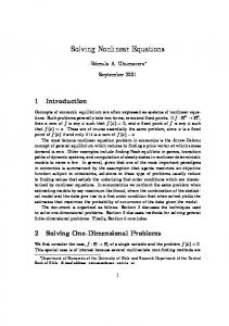
A third major group of online rotor resistance adaptation methods is based on principles of model reference adaptive control. The basic idea is that one quantity can be calculated in two different ways. The first value is calculated from references inside the control system. The second value is calculated from measured signals. One of the two values is independent of the rotor resistance (rotor time constant). The difference between the two is an error signal, which is assigned entirely to the error in rotor resistance used in the control system. The error signal is used to drive an adaptive mechanism (PI or I controller) which provides correction of the rotor resistance (Figure 2.1). Any method that belongs to this group utilizes the machine’s model, so its accuracy is heavily dependent on the accuracy of the applied model. This is the approach that has attracted most of the attention due to its relatively simple implementation requirements. In [53], four different reference models were proposed. According to the different physical quantities which are selected for adaptation purposes, this group of methods can be divided into several categories. The reactive power-based method is not dependent on stator resistance at all and is probably the most frequently applied

16

Inputs

Input Decoupling &Scaling

Induction machine

Measurement Outputs

Adaptive Terms

Model Reference Error Reference Machine Model

Adaptive Controller

+ Coherent Power of Model Reference Error

Figure 2.1: The structure of model reference adaptive system-based method

17

approach (see [54], [55], [56], [53] and [57]). Other possibilities include selection of torque [53], [58], rotor back emf [59], [60], rotor flux magnitude [53], rotor flux d-, and q-components [61], stored magnetic energy [62], product of stator q-axis current and rotor flux [63], stator fundamental RMS voltage [64], stator d-axis or q-axis voltage components [63], or stator q-axis current component [65]. There are a couple of common features that all of the methods of this group share. First, rotor resistance adaptation is usually operational in steady-states only and is then disabled during transients. Thus, the adaptation can be based on steady-state model of the machine. Second, in the vast majority of cases, stator voltages are required for calculation of the adaptive quantity, and they have to be either measured or reconstructed from the inverter firing signals and measured DC link voltage. Third, in most cases, identification does not work at zero speed and at zero load torque. Finally, identification heavily relies on the model of the machine, in which, most frequently, all of the other parameters are treated as constants. This is at the same time the major drawback of this group of methods. Indeed, an analysis of the influence of parameter variation on the accuracy of rotor resistance adaptation [66] shows that when rotor flux magnitude method is applied and actual leakage inductances deviate by 40% from the values used in the adaptation, rotor resistance is estimated with such an error that the response of the drive becomes worse than with no adaptation at all. A similar study, with very much the same conclusions, is described in [67] where parameter sensitivity is examined for d-axis stator voltage method, q-axis stator voltage method, air gap power method, and reactive power method. The different reference model algorithms have certain advantages and limitations if they are compared in the areas of convergence, load dependency and sensitivity to detuning. Thus, depending on the application, any one of them may be the most 18

suitable. On the other hand, none of them will provide a total solution to the detuning problem.

2.3.5

Other methods

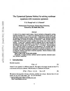
There exist a number of other possibilities for online rotor resistance (rotor time constant) adaptation, such as those described in [68], [69] and [70]. For example, the method of [70] does not require either a special test signal or complex computations. It is based on a special switching technique of the current regulated PWM inverter, which allows measurement of the induced voltage across the disconnected stator phase. The rotor time constant is then identified directly from this measured voltage and measured stator currents. The technique provides up to six windows within one electric cycle to update the rotor time constant, which is sufficient for all practical purposes. Another possibility, opened up by the recent developments in the area of artificial intelligence (AI), is the application of artificial neural networks for the online rotor time constant (rotor resistance) adaptation (Figure 2.2). Such a possibility is explored in [71], [72], [73], [74], [75]. The other AI technique that can be utilized for online rotor time constant adaptation is fuzzy logic [76], [77], [78]. Recent emphasis on sensorless vector control has led to a development of a number of schemes for simultaneous rotor speed and rotor time constant online estimation, that are applicable in conjunction with the appropriate speed estimation model-based algorithms [79], [80], [81]. These methods of rotor time constant estimation mostly belong to one of the groups already reviewed in this section.

19

usa usb

isa

Induction Machine

isb ω

Estimated Rotor Time Constant Neural Network Figure 2.2: The structure of artifical neural network method

20

2.4

Online Estimation of Stator Resistance

An industrially accepted standard for sensored rotor flux oriented control has become the indirect rotor flux oriented control (IRFOC), which does not require the knowledge of the stator resistance. Since the rotor time constant is of crucial importance for decoupled flux and torque control in IRFOC, the major effort was directed toward development of online techniques for rotor time constant identification. The situation has however dramatically changed with the advent of sensorless vector control, which involves rotor speed estimation. A vast majority of speed estimation techniques are based on the induction machine model and involve the stator resistance as a parameter in the process of speed estimation. An accurate value of the stator resistance is of utmost importance in this case for correct operation of the speed estimator in the low speed region. If stator resistance is detuned, large speed estimation errors and even instability at very low speeds result. It is for this reason that online estimation of stator resistance has received considerable attention during the last decade. There are a large number of publications devoted to this subject, [82], [83], [84]. The other driving force behind the increased interest in online stator resistance estimation was the introduction of direct torque control (DTC), which in its basic form relies on estimation of stator flux from measured stator voltages and currents. The accuracy of DTC, especially in the low frequency region, therefore heavily depends on the knowledge of the correct stator resistance value. In general, methods of stator resistance estimation are similar to those utilized for rotor time constant (rotor resistance) estimation and include application of observers, extended Kalman filters, model reference adaptive systems, and artificial intelligence.

21

2.5

Combination of Parameter Identification and Velocity Estimation

A combined parameter identification and velocity estimation problem is discussed in [32], [85] and [86]. The methodology in [86] requires a constant or slowly varying speed. In this thesis, the velocity estimation problem is not considered, but the velocity is allowed to vary.

2.6

Summary

This chapter reviews various techniques for tracking the rotor time constant. They can be divided into four main categories: (1) least-squares method, (2) spectral analysis method, (3) observer-based method, and (4) model reference adaptive system-based method.

22

Chapter 3 NONLINEAR LEAST-SQUARES APPROACH FOR PARAMETER IDENTIFICATION 3.1

Introduction

This work is concerned with the identification of the induction motor parameters. The induction motor is usually modeled as a set of five coupled nonlinear equations and there are such representations for which the model is linear in the parameters. In such a case, a standard least-squares criteria leads to a minimization of a quadratic cost function whose extrema equations are linear in the parameters. However, the rotor state-variables are not usually available measurements so that this standard linear least-squares approach does not apply. Here, the model of the machine is first written as a linear overparameterized system in which the rotor state-variables are not used. Next, the nonlinear relationships 23

between the parameters in the overparameterized model are taken into account in the expression for the residual error. The extrema equations for the residual error are then computed, which are nonlinear rational functions of the unknown parameters. Next, these rational (in the parameters) extrema equations are converted into equivalent polynomial equations by multiplying them through by their least common multiple. The equivalent polynomial equations are solved for all of their zeros using elimination theory (via resultants) and the roots that result in the minimum residual error are used to obtain the parameter values of the machine.

3.2

Induction Motor Model

The work here is based on standard models of induction machines available in the literature [87]. These models neglect parasitic effects such as hysteresis, eddy currents and magnetic saturation. The particular model formulation used here is the state space model of the system given by (cf. [88] [89]) dω dt dψ Ra dt dψ Rb dt diSa dt diSb dt

= = = = =

np M τL (iSb ψRa − iSa ψRb ) − JLR J 1 M − ψRa − np ωψ Rb + iSa TR TR 1 M − ψRb + np ωψ Ra + iSb TR TR 1 β ψRa + βnp ωψ Rb − γiSa + uSa TR σLS 1 β ψRb − βnp ωψ Ra − γiSb + uSb TR σLS

24

(3.1)

where ω = dθ/dt with θ the position of the rotor, np is the number of pole pairs, iSa , iSb are the (two phase equivalent) stator currents and ψRa , ψ Rb are the (two phase equivalent) rotor flux linkages. The induction motor parameters are the five electrical parameters, RS and RR (the stator and rotor resistances), M (the mutual inductance), LS and LR (the stator and rotor inductances), and the two mechanical parameters, J (the inertia of the rotor) and τ L (the load torque). The symbols TR =

β=

LR RR

M σLS LR

σ =1−

γ=

M2 LS LR

RS 1 1 M2 + σLS σLS TR LR

have been used to simplify the expressions. TR is referred to as the rotor time constant while σ is called the total leakage factor. This model is then transformed into a coordinate system attached to the rotor. For example, the current variables are transformed according to 









 iSx   cos(np θ) sin(np θ)   iSa   = .  − sin(np θ) cos(np θ) iSy iSb

(3.2)

The transformation simply projects the vectors in the (a, b) frame onto the axes of the moving coordinate frame. An advantage of this transformation is that the signals in the moving frame (i.e., the (x, y) frame) typically vary slower than those in the (a, b) frame (they vary at the slip frequency rather than at the stator frequency). At the same time, the transformation does not depend on any unknown parameter in contrast to the field-oriented d/q transformation. The stator voltages and the rotor 25

fluxes are transformed with the same method as the currents resulting in the following model ( [90]) diSx dt diSy dt dψ Rx dt dψ Ry dt dω dt

3.3

= = = = =

1 β uSx − γiSx + ψ + np βωψ Ry + np ωiSy σLS TR Rx 1 β uSy − γiSy + ψ − np βωψ Rx − np ωiSx σLS TR Ry 1 M iSx − ψ TR TR Rx 1 M iSy − ψ TR TR Ry τL np M (iSy ψRx − iSx ψRy ) − . JLR J

(3.3) (3.4) (3.5) (3.6) (3.7)

Linear Overparameterized Model

Measurements of the stator currents iSa , iSb and voltages uSa , uSb as well as the position θ of the rotor are assumed to be available (velocity may then be reconstructed from position measurements). However, the rotor flux linkages ψRx , ψ Ry are not assumed to be measured. Standard methods for parameter estimation are based on equalities where known signals depend linearly on unknown parameters. However, the induction motor model described above does not fit in this category unless the rotor flux linkages are measured. The first step is to eliminate the fluxes ψRx , ψ Ry and their derivatives dψ Rx /dt, dψ Ry /dt. The four equations (3.3), (3.4), (3.5), (3.6) can be used to solve for ψRx , ψ Ry , dψ Rx /dt, dψ Ry /dt, but one is left without another independent equation(s) to set up a regressor system for the identification algorithm. A new set of independent equations are found by differentiating equations (3.3) and

26

(3.4) to obtain dψ Ry 1 duSx dω d2 iSx β dψ Rx diSx = − − n − np βψRy + γ βω p 2 σLS dt dt dt TR dt dt dt dω diSy −np ω − np iSy dt dt

1 duSy dω diSy dψ d2 iSy β dψ Ry +γ = − + np βω Rx + np βψRx 2 σLS dt dt dt TR dt dt dt dω diSx +np ω + np iSx . dt dt

(3.8)

(3.9)

Next, equations (3.3), (3.4), (3.5), (3.6) are solved for ψRx , ψ Ry , dψ Rx /dt, dψ Ry /dt and substituted into equations (3.8) and (3.9) to obtain 1 duSx βM γ 1 diSx d2 iSx diSy + ) ) np ω + − (γ + − iSx (− 2 + 2 dt dt σLS dt TR dt TR TR 1 dω dω 1 βM uSx + )+ + np iSy − np × + iSy np ω( TR TR σLS TR dt dt σLS (1 + n2p ω2 TR2 ) µ diSy diSx − γiSy σLS TR − iSx np ωσLS TR − np ωσLS TR2 −σLS TR dt dt ´ 2 2 2 2 2 (3.10) −γiSx np ωσLS TR + iSy np ω σLS TR + np ωTR uSx + TR uSy

0=−

and 1 duSy βM γ 1 diSy d2 iSy diSx − ) ) np ω + − (γ + − iSy (− 2 + 2 dt dt σLS dt TR dt TR TR dω dω 1 1 βM uSy × + )+ − np iSx + np − iSx np ω( TR TR σLS TR dt dt σLS (1 + n2p ω 2 TR2 ) µ diSx diSy − γiSx σLS TR + iSy np ωσLS TR + np ωσLS TR2 −σLS TR dt dt ´ +γiSy np ωσLS TR2 + iSx n2p ω 2 σLS TR2 − np ωTR2 uSy + TR uSx (3.11)

0=−

27

The set of equations (3.10) and (3.11) may be rewritten in regressor form as

(3.12)

y(t) = W (t)K

where K ∈ R15 , W ∈ R2×15 and y ∈ R2 are given by K ,

·

γ βM

TR2

γTR2

1 σLS

βM TR2

1 TR

TR2 σLS

1 σLS TR

γ TR TR σLS

βM TR

TR γTR βMTR

¸T



diSx diSx duSx 2 2 iSx np ωiSy − −iSx np ωiSy  − dt np ω iSx dt dt W (t) ,  di duSy diSy Sy n2p ω 2 iSy iSy −np ωiSx − −iSy −np ωiSx − dt dt dt diSx diSy dω dω + n3p ω3 iSy + (np + n2p ωiSx ) − n2p ω 2 iSx −n2p ω 2 np iSy n3p ω3 iSy dt dt dt dt diSy diSx dω dω −n2p ω 2 − n3p ω 3 iSx + (−np + n2p ωiSy ) −np iSx − n2p ω2 iSy −n3p ω3 iSx dt dt dt dt diSx dω dω d2 iSx diSy dω diSx duSx − ω 2 2 ) + n3p ω 3 n2p (ωiSx − ω2 ) n2p (ω2 − uSx ω ) n2p (ω dt dt dt dt dt dt dt dt 2 dω diSy dω dω 2 2 d iSy 3 3 diSx 2 2 diSy 2 2 duSy np (ω ) − np ω −ω np (ωiSy −ω ) np (ω − uSy ω ) dt dt dt2 dt dt dt dt dt  dω uSx n2p ω2 uSx − np uSy dt  dω  2 2 uSy np ω uSy + np uSx dt and



d2 iSx dω diSy  dt2 − np iSy dt − np ω dt  y(t) ,    2 d iSy diSx dω + np ω + np iSx 2 dt dt dt

28



  .  

Though the system (3.12) is linear in the parameters, it is overparameterized resulting in poor numerical conditioning if standard least-squares techniques are used. Specifically,

K1 = K6 K8 , K2 = K4 K82 , K3 = K8 K14 , K5 = 1/K8 , K7 = K4 K8 , K9 = K6 K82 K10 = K4 K83 , K11 = K82 , K12 = K6 K83 , K13 = K14 K83 , K15 = K14 K82

(3.13)

so that only the four parameters K4 , K6 , K8 , K14 are independent. Also, not all five electrical parameters RS , LS , RR , LR and M can be retrieved from the Ki ’s. The four parameters K4 , K6 , K8 , K14 determine only the four independent parameters RS , LS , σ and TR by

RS =

K6 − K4 1 + K4 K82 1 , TR = K8 , LS = ,σ = . K14 K14 K8 1 + K4 K82

(3.14)

As TR = LR /RR and σ = 1 − M 2 / (LS LR ), only LR /RR and M 2 /LR can be obtained, and not M, LR , and RR independently. This situation is inherent to the identification problem when rotor flux linkages are unknown and is not specific to the proposed method. If the rotor flux linkages are not measured, machines with different RR , LR , and M, but identical LR /RR and M 2 /LR will have the same input/output (i.e., voltage to current and speed) characteristics. Specifically, the transformation ratio from stator to rotor cannot be determined unless rotor measurements are taken. However, machines with different Ki parameters, yet satisfying the nonlinear relationships (3.13), will be distinguishable. For a related discussion of this issue, see Bellini et al [91] where parameter identification is performed using torque-speed and stator current-speed characteristics.

29

3.4

Least-Squares Identification

Equation (3.12) can be rewritten in discrete time as

(3.15)

y(n) = W (n)K

where n is the time instant at which a measurement is taken and K is the vector of unknown parameters. If the constraint (3.13) is ignored, then the system is a linear least-squares problem. To find a solution for such a system, the least-squares algorithm is used. Specifically, given y(n) and W (n) where y(n) = W (n)K, one defines E 2 (K) ,

N ¯ ¯2 X ¯ ¯ y(n) − W (n)K ¯ ¯

(3.16)

n=1

as the residual error associated to a vector K. Then, the least-squares estimate K ∗ is chosen such that E 2 (K) is minimized for K = K ∗ . The function E 2 (K) is quadratic and therefore has a unique minimum at the point where ∂E 2 (K)/∂K = 0. Solving this expression for K ∗ yields the standard least-squares solution to y(n) = W (n)K given by ∗

K =

"N X n=1

#−1 " N # X T W (n)W (n) W (n)y(n) . T

(3.17)

n=1

Define

RW =

N X n=1

W T (n)W (n), RW y =

N X

W T (n)y(n), Ry =

n=1

so that −1 RW y . K ∗ = RW

30

N X n=1

y T (n)y(n).

For our identification problem, it is to minimize N ¯ ¯2 X ¯ ¯ T T E (K) = ¯y(n) − W (n)K ¯ = Ry − 2RW y K + K RW K 2

(3.18)

n=1

subject to the constraints

K1 = K6 K8 , K2 = K4 K82 , K3 = K8 K14 , K5 = 1/K8 , K7 = K4 K8 , K9 = K6 K82 K10 = K4 K83 , K11 = K82 , K12 = K6 K83 , K13 = K14 K83 , K15 = K14 K82 .

(3.19)

On physical grounds, the parameters K4 , K6 , K8 , K14 are constrained to

0 < Ki < ∞ for i = 4, 6, 8, 14.

(3.20)

Also, based on physical grounds, the squared error E 2 (K) will be minimized in the interior of this region. Let N ¯ ¯2 ¯ X ¯ ¯ ¯ T E (Kp ) , ¯y(n) − W (n)K ¯K1 =K6 K8 = Ry − 2RW y K ¯ 2

n=1

K1 =K6 K8 K2 =K4 K82

K2 =K4 K82

.. .

where Kp ,

·

K4 K6 K8 K14

¸T

.. .

¡ T ¢¯¯ + K RW K ¯

K1 =K6 K8 K2 =K4 K82

.. . (3.21)

.

As just explained, the minimum of (3.21) must occur in the interior of the region and therefore at an extremum point.

31

This then entails solving the four equations ∂E 2 (Kp ) ∂K4 ∂E 2 (Kp ) r2 (Kp ) , ∂K6 ∂E 2 (Kp ) r3 (Kp ) , ∂K8 ∂E 2 (Kp ) r4 (Kp ) , ∂K14 r1 (Kp ) ,

=0

(3.22)

=0

(3.23)

=0

(3.24)

= 0.

(3.25)

The partial derivatives in (3.22)-(3.25) are rational functions in the parameters K4 , K6 , K8 , K14 . Defining ∂E 2 (Kp ) ∂K4 ∂E 2 (Kp ) p2 (Kp ) , K8 r2 (Kp ) = K8 ∂K6 ∂E 2 (Kp ) p3 (Kp ) , K83 r3 (Kp ) = K83 ∂K8 ∂E 2 (Kp ) p4 (Kp ) , K8 r4 (Kp ) = K8 ∂K14

p1 (Kp ) , K8 r1 (Kp ) = K8

(3.26) (3.27) (3.28) (3.29)

results in the pi (Kp ) being polynomials in the parameters K4 , K6 , K8 , K14 and having the same positive zero set (i.e., the same roots satisfying Ki > 0) as the system (3.22)-(3.25). The degrees of the polynomials pi are given in Table 3.1. All possible solutions to this set may be found using elimination theory as is now summarized.

32

Table 3.1: The degrees of the polynomials pi deg K4 deg K6 deg K8 deg K14 p1 (Kp ) 1 1 7 1 p2 (Kp ) 1 1 7 1 p3 (Kp ) 2 2 8 2 p4 (Kp ) 1 1 7 1

33

3.4.1

Solving systems of polynomial equations

The question at hand is “Given two polynomial equations a(K1 , K2 ) = 0 and b(K1 , K2 ) = 0, how does one solve them simultaneously to eliminate (say) K2 ?". A systematic procedure to do this is known as elimination theory and uses the notion of resultants. Briefly, one considers a(K1 , K2 ) and b(K1 , K2 ) as polynomials in K2 whose coefficients are polynomials in K1 . Then, for example, letting a(K1 , K2 ) and b(K1 , K2 ) have degrees 3 and 2, respectively in K2 , they may be written in the form a(K1 , K2 ) = a3 (K1 )K23 + a2 (K1 )K22 + a1 (K1 )K2 + a0 (K1 ) b(K1 , K2 ) = b2 (K1 )K22 + b1 (K1 )K2 + b0 (K1 ).

The n × n Sylvester matrix, where n = degK2 {a(K1 , K2 )} + degK2 {b(K1 , K2 )} = 3 + 2 = 5, is defined by 

a0 (K1 )

   a1 (K1 )   Sa,b (K1 ) ,   a2 (K1 )    a3 (K1 )  0

0

b0 (K1 )

a0 (K1 ) a1 (K1 ) a2 (K1 ) a3 (K1 )

0

0



   b1 (K1 ) b0 (K1 ) 0   b2 (K1 ) b1 (K1 ) b0 (K1 )  .   0 b2 (K1 ) b1 (K1 )   0 0 b2 (K1 )

(3.30)

The resultant polynomial is then defined by ³ ´ r(K1 ) = Res a(K1 , K2 ), b(K1 , K2 ), K2 , det Sa,b (K1 )

(3.31)

and is the result of eliminating the variable K2 from a(K1 , K2 ) and b(K1 , K2 ). In fact, the following is true. 34

Theorem 1 [92] [93] Any solution (K10 , K20 ) of a(K1 , K2 ) = 0 and b(K1 , K2 ) = 0 must have r(K10 ) = 0. Though the converse of this theorem is not necessarily true, the finite number of solutions of r(K1 ) = 0 are the only possible candidates for the first coordinate (partial solutions) of the common zeros of a(K1 , K2 ) and b(K1 , K2 ). Whether or not such a partial solution extends to a full solution is easily determined by back solving and checking the solution (See the Appendix). Using the polynomials (3.26)-(3.29) and the computer algebra software program Mathematica [94], the variable K4 is eliminated first to obtain three polynomials in three unknowns as ´ ³ rp1p2 (K6 , K8 , K14 ) , Res p1 (K4 , K6 , K8 , K14 ), p2 (K4 , K6 , K8 , K14 ), K4 ´ ³ rp1p3 (K6 , K8 , K14 ) , Res p1 (K4 , K6 , K8 , K14 ), p3 (K4 , K6 , K8 , K14 ), K4 ´ ³ rp1p4 (K6 , K8 , K14 ) , Res p1 (K4 , K6 , K8 , K14 ), p4 (K4 , K6 , K8 , K14 ), K4 and the degrees of the polynomials are given in Table 3.2. Next K6 is eliminated to obtain two polynomials in two unknowns as ³ ´ rp1p2p3 (K8 , K14 ) , Res rp1p2 (K6 , K8 , K14 ), rp1p3 (K6 , K8 , K14 ), K6 ´ ³ rp1p2p4 (K8 , K14 ) , Res rp1p2 (K6 , K8 , K14 ), rp1p4 (K6 , K8 , K14 ), K6 and the degrees of these two polynomials are given in the Table 3.3. Finally K14 is eliminated to obtain a single polynomial in K8 as ´ ³ r(K8 ) , Res rp1p2p3 (K8 , K14 ), rp1p2p4 (K8 , K14 ), K14 35

Table 3.2: The degrees of the polynomials rp1p2 , rp1p3 , rp1p4 deg K6 deg K8 deg K14 rp1p2 1 14 1 rp1p3 2 22 2 rp1p4 1 14 1

Table 3.3: The degrees of the polynomials rp1p2p3 , rp1p2p4 deg K8 deg K14 rp1p2p3 50 2 rp1p2p4 28 1

36

where deg K8 = 104. The parameter K8 was chosen as the variable not eliminated because its degree was the highest at each step meaning it would have a larger (in dimension) Sylvester matrix than using any other variable. The positive roots of r(K8 ) = 0 are found which are then substituted into rp1p2p3 = 0 (or rp1p2p4 = 0) which in turn are solved to obtain the partial solutions (K8 , K14 ). The partial solutions (K8 , K14 ) are then substituted into rp1p2 = 0 (or rp1p3 = 0 or rp1p4 = 0) which are solved to obtain the partial solutions (K6 , K8 , K14 ) so that they in turn may be substituted into p1 = 0 (or p2 = 0 or p3 = 0 or p4 = 0) which are solved to obtain the solutions (K4 , K6 , K8 , K14 ). These solutions are then checked to see which ones satisfy the complete system of polynomials equations (3.26)-(3.29), and those that do constitute the candidate solutions for the minimization. Based on physical considerations, the set of candidate solutions is non empty. From the set of candidate solutions, the one that gives the smallest squared error is chosen. Computational issues Due to the high degrees of the resultant polynomials, care must be taken to compute their roots. The data is collected and brought into Mathematica [94]. The matrices Ry , RW , RW y are then computed and their entries converted to rational form. Finally the roots of the resultant polynomials are computed in Mathematica using rational arithmetic with 16 digits of precision.

37

Numerical conditioning of the nonlinear least-squares solution After finding the solution that gives the minimal value for E 2 (Kp ), one needs to know if the solution makes sense. For example, in the linear least-squares problem, there is a unique well defined solution provided that the regressor matrix RW is nonsingular (or in practical terms, its condition number is not too large). In the nonlinear case here, a ∗ T ] Taylor series expansion about the computed minimum point Kp∗ = [K4∗ , K6∗ , K8∗ , K14

to obtain (i, j = 4, 6, 8, 14)

E 2 (Kp ) = E 2 (Kp∗ ) +

¤T ∂ 2 E 2 (Kp∗ ) £ ¤ 1£ Kp − Kp∗ Kp − Kp∗ + · · · . 2 ∂Ki ∂Kj

(3.32)

One then checks that the Hessian matrix ∂ 2 E 2 (Kp∗ )/∂Ki ∂Kj is positive definite as well as its condition number to ensure that the data is sufficiently rich to identify the parameters.

3.4.2

Error estimates

Residual error index To develop a measure of how well the data y(n) fits W T (n)K ∗ , one defines the residual error at K ∗ as

N ¯ ¯2 X ¯ T ∗¯ T ∗ ∗T ∗ E (K ) = ¯y(n) − W (n)K ¯ = Ry − 2RW y K + K RW K 2

∗

n=1

38

(3.33)

Note that 0 ≤ E 2 (K ∗ ) ≤ Ry . Next, define the residual error index to be (see [33]) EI =

s

E 2 (K ∗ ) Ry

(3.34)

which is zero when E 2 (K ∗ ) = 0 (or y(n) = W T (n)K ∗ for all n), and 1 when K ∗ = 0 (or E 2 (K ∗ ) = Ry ). Therefore, the residual error index EI ranges from 0 to 1, where EI = 0 indicates that y(n) fits the relationship W T (n)K ∗ perfectly. The residual error index EI is usually nonzero due to noise, unmodeled dynamics and nonlinearities. In the worst case, EI = 1, which would mean that the residual error has a magnitude comparable to that of the measurement y(n). Parametric error indices In addressing the issue of sensitivity of K ∗ to errors, recall that at K = K ∗ ·

∂E 2 (K) ∂K

¸

= 0.

K=K ∗

Therefore, it is not possible to use the derivative of the residual error as a measure of how sensitive the error is with respect to K. An alternative is to define δK as the variation in K such that the increase of error is equal to some times, say, two times the residual error E 2 (K ∗ ) (see Figure 3.1). Recalling (3.33),

T T ∗ ∗ ∗ E 2 (K ∗ + δK) = Ry − 2RW y (K + δK) + (K + δK) RW (K + δK)

39

(3.35)

E 2 (K * +δK )

2E 2 (K *) E 2 ( K *) K * −δK

K*

K * +δK

Figure 3.1: E 2 (K ∗ + δK) versus δK

40

The parametric error index δK1 associated with the parameter K1 , is defined as the maximum value of δK1 such that E 2 (Kp∗ + δKp ) = CE 2 (Kp∗ ), where C is a constant

is satisfied. In our problem, the parametric error index is chosen as the maximum value of δKi for i = 4, 6, 8, 14 such that E 2 (Kp∗ + δKp ) = 1.25E 2 (Kp∗ ) where δKp ,

·

δK4 δK6 δK8 δK14

¸T

(3.36)

. In words, for all δKp that result in a

25% increase in the residual error, find the maximum value of δKi for i = 4, 6, 8, 14. Mathematically, one maximizes

δKi where i = 4, 6, 8, or 14

subject to (3.36). This is straightforwardly setup as an unconstrained optimization using Lagrange multipliers by maximizing ³ ´ δKi + λ E 2 (Kp∗ + δKp ) − 1.25E 2 (Kp∗ ) over all possible δKp ,

·

δK4 δK6 δK8 δK14

the extrema are solutions to

41

¸T

(3.37)

and λ. For example, with i = 4,

¡ ¢ ∂ E 2 (Kp∗ + δKp ) − 1.25E 2 (Kp∗ ) 1+λ ∂δK4 ¢ ¡ 2 ∗ ∂ E (Kp + δKp ) − 1.25E 2 (Kp∗ ) λ ∂δK6 ¡ 2 ∗ ¢ ∂ E (Kp + δKp ) − 1.25E 2 (Kp∗ ) λ ∂δK8 ¡ 2 ∗ ¢ ∂ E (Kp + δKp ) − 1.25E 2 (Kp∗ ) λ ∂δK14

= 0

(3.38)

= 0

(3.39)

= 0

(3.40)

= 0

(3.41)

E 2 (Kp∗ + δKp ) − 1.25E 2 (Kp∗ ) = 0.

(3.42)

The equations (3.38) through (3.42) are transformed to five polynomial equations in the five unknowns δK4 , δK6 , δK8 , δK14 , and λ, and elimination theory is used to solve this system. A large parametric error index indicates that the parameter estimate could vary greatly without a large change in the residual error. Thus, the accuracy of the parameter estimates would be in doubt. Likewise, a small parametric error indicates that the residual error is very sensitive to changes in the parameter estimates. In such cases, the parameter estimates may be considered more accurate. In any case, the error indices should not be considered as actual errors, but rather as orders of magnitude of the errors to be expected, to guide the identification process and to warn about unreliable results. Obviously, the choice of a parametric error index is somewhat subjective. A different level of residual error would lead to a scaling of all the components of the parametric error index by a common factor. An alternative would be to select a residual error level corresponding to a known bound on the measurement noise (thus the algorithm of [95]). While such an assumption leads to rigorous bounds on the 42

parametric errors, the noise bound itself would still be highly subjective as it would have to account for modelling errors as well as measurement noise.

3.4.3

Mechanical parameters

Once the electrical parameters have been found, the two mechanical parameters J, f (τ L = −fω) can be found using a linear least-squares algorithm. To do so, equations (3.8) and (3.9) are solved for Mψ Rx /LR , Mψ Ry /LR resulting in 







1  1/TR −ω   Mψ Rx /LR   = σLS    2 (1/TR ) + n2p ω 2 Mψ Ry /LR ω 1/TR    diSx /dt − uSx / (σLS ) + γiSx − np ωiSy  × . diSy /dt − uSy / (σLS ) + γiSy + np ωiSx

(3.43)

Noting that

γ=

RS 1 1 M2 RS 1 1 + = + (1 − σ) LS , σLS σLS TR LR σLS σLS TR

(3.44)

it is seen that the quantities on the right hand side of (3.43) are all known once the electrical parameters have been computed. With K16 , np /J, K17 , f /J, equation (3.7) may be rewritten as

dω = dt

·

Mψ Ry Mψ Rx iSy − iSx LR LR

43



¸  K16  −ω    K17

     

so that the standard linear squares approach of Section 3.4 is directly applicable. Then J , np /K16 , f , np K17 /K16 .

3.5

(3.45)

Simulation Results

The algorithm was first applied to simulated “data” to see how it performs under ideal conditions. In particular, the simulations are helpful in evaluating the usefulness of the parametric error indices. Here, a two pole-pair (np = 2), three-phase induction motor model was simulated using Simulink with parameter values chosen to be

RS = 9.7 Ω, RR = 8.6 Ω, LS = LR = 0.67 H, M = 0.64 H, σ = 0.088, J = 0.011 kgm2 , τ L = 3.7 Nm.

A 2048 pulse/rev position encoder and 12 bit A/D converters were included in the simulation model in order to more accurately represent the physical system. These values correspond to a 1/2 kW machine with a synchronous frequency of 50 Hz. These machine parameter values correspond to the following K values

K1 = 299.15, K2 = 10.42, K3 = 17.05, K4 = 1717.18, K5 = 12.84 K6 = 3839.8, K7 = 133.78, K8 = 0.0779, K9 = 23.31, K10 = 0.8120 K11 = 0.0061, K12 = 1.82, K13 = 0.1035, K14 = 218.83, K15 = 1.328

44

for the electrical parameters and to

K16 = 181.82, K17 = 336.36

for the mechanical parameters. Figure 3.2 shows the simulated speed response (from standstill) of the induction motor when a balanced (open loop) set of three phase voltages of amplitude 466.7 Volts (line-line) and frequency 50 Hz were applied to the machine. The constant load torque causes the machine to rotate in the opposite direction at the beginning of the operation. The data {uSa , uSb , iSa , iSb , θ} was collected between 0 sec and 0.2 sec. The quantities uSx , uSy , duSx /dt, duSy /dt, iSx , iSy diSx /dt, diSy /dt, d2 iSx /dt2 , d2 iSy /dt2 , ω = dθ/dt, dω/dt were calculated, and the regressor matrices RW , Ry and RW y were computed. The procedure explained in Section 3.4.1 was then carried out to compute K4 , K6 , K8 , K14 . In this case, there was only one extremum point that had positive values for all the Ki . Table 3.4 compares the electrical parameter values determined from the nonlinear least-squares procedure to their actual values (which are known only because this is simulation data). Also given in the table are the corresponding parametric error indices. The residual error index for the parameters K4 , K6 , K8 , K14 was computed to be 3.15%, and it is small. Using these values, the scaled flux linkages Mψ Rx /LR , Mψ Ry /LR were reconstructed according to (3.43) to estimate the mechanical parameters K16 , K17 . Table 3.5 compares the mechanical parameter values determined from the least-squares procedure to their actual values along with the corresponding parametric error indices.

45

Speed Versus Time

160 140

Speed in radians/sec

120 100 80 60 40 20 0

-20

0

0.05

0.1

0.15

Time in seconds

Figure 3.2: Rotor speed versus time.

46

0.2

Table 3.4: The electrical parameter values

∗

Parameter

True Value

Estimated Value

Parametric Error Index with 1.25E 2 (K p )

K4 K6 K8 K14

1717.2 3839.8 0.0779 218.8

1743.4 3917.5 0.0780 222.2

13.23 24.59 0.00031 8.27

Table 3.5: The mechanical parameter values

∗

Parameter

True Value

Estimated Value

Parametric Error Index with 1.25E 2 (K p )

K16 K17

181.8 336.4

195.3 359.3

4.29 9.78

47

The residual error index for the mechanical parameters K16 , K17 was computed to be 4.26%, and it is small. The Hessian matrix for the identification of the parameters K4 , K6 , K8 , K14 was calculated at the minimum point according to (3.32) resulting in 

40.33 −89.39  7.534 0.2175  ½ 2 2 ∗ ¾  10.17 −44.35 ∂ E (Kp )  0.2175 18.04 =  40.33 ∂Ki ∂Kj 10.17 5.308 × 104 1.112 × 103   −89.39 −44.35 1.112 × 103 1.876 × 103

        

which is positive definite and has a condition number of 1.88 × 104 . The Hessian matrix is well-conditioned, and it ensures numerical reliability of the computations. There are four positive eigenvalues for this Hessian matrix. The direction where the error function is most sensitive to the parameter change is given by the eigenvector corresponding to the biggest eigenvalue, whereas the direction where the error function is least sensitive is given by the eigenvector corresponding to the smallest value. Table 3.6 compares the estimated machine parameters to their actual values.

Table 3.6: The machine parameter values Parameter

True Value

Estimated Value

TR σ LS RS J τL

0.0779 sec 0.088 0.67 H 9.7 Ohms 0.011 kgm2 3.7 Nm

0.0780 sec 0.086 0.6698 H 9.8 Ohms 0.010 kgm2 3.68 Nm

48

3.6

Estimation of TR and RS for Online Update

During normal operation of the induction machine, the field oriented control requires knowledge of the rotor time constant TR = LR /RR (which varies significantly due to Ohmic heating) in order to estimate the rotor flux linkages. The interest here is in tracking the value of TR as it changes due to Ohmic heating so that an accurate value is available to estimate the flux for a field oriented controller. However, the stator resistance value RS will also vary due to Ohmic heating so that it must also be taken into account. The electrical parameters M, LS , σ are assumed to be known and not varying. Measurements of the stator currents iSa , iSb and voltages uSa , uSb as well as the position θ of the rotor are assumed to be available (velocity may then be reconstructed from position measurements). However, the rotor flux linkages are not assumed to be measured. From equations (3.10) and (3.11), if we assume the electrical parameters M, LS , σ are known, this set of equations may be rewritten in regressor form as

y(t) = W (t)K

where y ∈ R2 , W ∈ R2×8 and K ∈ R8 are given by 

 dω diSy duSx /dt d2 iSx 2 2 − np ω − np ω MβiSx − − np iSy  2 dt dt σLs  y ,  dt  2 dω d iSy diSx dv Sy /dt 2 2 + n i ω ω Mβi − + n − n p Sx p Sy p dt2 dt dt σLs

49

(3.46)



diSx uSx diSx  − dt − dt + np ωiSy + np ωMβiSy + σLs MβiSx −iSx W =  di uSy diSy Sy − − − np ωiSx − np ωMβiSx + MβiSy −iSy dt dt σLs diSy dω dω diSx dω 1 np + n2p (ωiSx − ω2 ) + n3p ω 3 iSy (1 + Mβ) + (n2p ω 2 uSx − np uSy ) dt dt dt dt σLs dt diSx dω dω dω 1 2 2 diSy 3 3 2 2 + np (ωiSy −ω ) − np ω iSx (1 + Mβ) + (np ω uSy + np uSx ) −np dt dt dt dt σLs dt dω di dω Sx np iSy − n2p ω 2 iSx n2p (isx ω − ω2 ) dt dt dt (3.47) dω diSy dω − n2p ω 2 iSy n2p (isy ω − ω2 ) −np iSx dt dt dt  2 n2p dω diSx dω diSy 3 3 2 2 d iSx 2 duSx np (ω )+ −ω nω − (ωuSx −ω ) dt dt dt2 dt p σLs dt dt   2 2 np dω diSy dω diSx 3 3 2 2 d iSy 2 duSy )− −ω nω − (ωuSy −ω ) np (ω dt dt dt2 dt p σLs dt dt and K,

·

1 γ TR

1 TR2

γ TR γTR γTR2 TR2 TR

¸T

.

(3.48)

As M2 = (1 − σ) LS , Mβ = (1 − σ)/σ LR RS 1 1 M2 RS 1 1 γ = + = + (1 − σ) LS σLS σLS TR LR σLS σLS TR it is seen that y and W depend only on known quantities, while the unknowns RS and TR are contained only within K. Though the system regressor is linear in the parameters, one cannot use standard least-squares techniques because the system is overparameterized. Specifically,

K3 = K22 , K4 = K1 K2 , K5 = 1/K2 , K6 = K1 /K2 , K7 = K1 /K22 , K8 = 1/K22

50

(3.49)

so that only the two parameters K1 and K2 are independent. These two parameters determine RS and TR by

TR = 1/K2 RS = σLS K1 − (1 − σ)LS K2 .

(3.50)

Based on the same analysis as before, an expression (3.51) only including K1 and K2 can be obtained N ¯ ¯2 X ¯ ¯ E (Kp ) , ¯y(n) − W (n)K ¯ K 2

2 3 =K2 K4 =K1 K2

n=1

¯ ¯ T = Ry − 2RW K y ¯

.. .

+

K3 =K22 K4 =K1 K2

where Kp ,

·

.. .

K1 K2

¡ T ¢¯¯ K RW K ¯

(3.51)

K3 =K22 K4 =K1 K2

¸T

.. .

.

The minimum of (3.51) must occur in the interior of the region and therefore at an extremum point. This then entails solving the two equations ∂E 2 (Kp ) =0 ∂K1 ∂E 2 (Kp ) r2 (Kp ) , = 0. ∂K2 r1 (Kp ) ,

51

(3.52) (3.53)

The partial derivatives in (3.52)-(3.53) are rational functions in the parameters K1 , K2 . Defining

=

∂E K24

2

(Kp ) ∂K1 2 ∂E (Kp ) p2 (Kp ) , K25 r2 (Kp ) = K25 ∂K2

p1 (Kp ) ,

K24 r1 (Kp )

(3.54) (3.55)

results in the pi (Kp ) being polynomials in the parameters K1 , K2 and having the same positive zero set (i.e., the same roots satisfying Ki > 0) as the system (3.52)-(3.53). The degrees of the polynomials pi are given in Table 3.7. Using the polynomials (3.54)-(3.55), the variable K1 is eliminated to obtain ´ ³ r(K2 ) , Res p1 (K1 , K2 ), p2 (K1 , K2 ), K1

(3.56)

where degK2 {r(K2 )} = 20. The parameter K2 was chosen as the variable not eliminated because its degree is much higher than K1 , meaning it would have a larger (in dimension) Sylvester matrix. The positive roots of r(K2 ) = 0 are found which are then substituted into p1 = 0 (or p2 = 0) to find the positive roots in K1 , etc. The previous machine model was tested here again. The parameter values correspond to the following K values

K1 = 297.56, K2 = 12.84.

Table 3.7: The degrees of the ploynomials p1 , p2 deg K1 deg K2 p1 (Kp ) 1 7 p2 (Kp ) 2 8 52

Table 3.8 compares K1 and K2 values determined from the nonlinear least-squares procedure to their actual values from the simulation model. Also given in the table are the corresponding parametric error indices. The residual error index for the parameters K1 , K2 was computed to be 2.83%, which shows the estimation is good. The Hessian matrix for the identification of the parameters K1 and K2 was calculated at the minimum point according to (3.32) resulting in ½

2

2

¾ (Kp∗ )

∂ E ∂Ki ∂Kj



 =

∂ 2 E 2 (Kp∗ ) ∂K12

∂ 2 E 2 (Kp∗ ) ∂K1 ∂K2

∂ 2 E 2 (Kp∗ ) ∂K1 ∂K2

∂ 2 E 2 (Kp∗ ) ∂K22







  0.4213 0.00589   = 0.00589 113.8

(3.57)

which is positive definite and has a condition number of 276. This shows the Hessian matrix is well-conditioned, and it ensures numerical reliability of the computations. The eigenvalues of the Hessian matrix are 113.8 and 0.42. As we mentioned before, the eigenvector corresponding to the biggest eigenvalue 113.8 gives the direction where the error function is most sensitive, whereas the eigenvector corresponding to the smallest value 0.42 gives the direction where the function is least sensitive. Table 3.9 compares the estimated machine parameters (TR and RS ) to their actual values.

3.7

Summary

This chapter presents the proposed approach for identifying the induction machine parameters. The methodology begins with an input-output linear overparameterized model whose parameters are rationally related. After making appropriate substitutions that account for the overparameterization, the problem is transformed into a nonlinear least-squares problem that is not overparameterized. The extrema equations can be solved using elimination theory. 53

Table 3.8: The estimated values and true values of K1 and K2 ∗ True Value Estimated Value Parametric Error Index with 1.25E 2 (K p ) 297.56 298.06 3.46 12.84 12.82 0.85

Parameter

K1 K2

Table 3.9: The estimated values and true values of TR and RS Parameter

True Value

Estimated Value

TR RS

0.0779 sec 9.70 Ohms

0.0780 sec 9.74 Ohms

54

Chapter 4 OFFLINE EXPERIMENTAL RESULTS 4.1

Introduction

In the previous chapter, the simulation results show the algorithm generates correct estimate for the induction machine parameters. The next step is to setup the equipment and run the induction machine with open loop control. This chapter will present the offline experimental results.

4.2

Experiment Setup

The data acquisition and control algorithms were implemented on the RT-LAB realtime platform. RT-LAB is a software package that allows the user to readily convert Simulink models to real-time simulations, via Real-Time Workshop (RTW), and run them over one or more processors. This is used particularly for Hardware-in-the-loop

55

(HIL) and rapid control prototyping applications. In our experiment configuration, there is one target computer running the control logic and one command station connecting to the target via Ethernet link. The target runs QNX, the real-time operating system software, and it has dual CPUs on the motherboard. The HIL I/O interface is installed on the target machine. It includes a 16-channel A/D module, an 8-channel D/A module, a quad-decoder module for shaft position measurement and a hardware clock. (Figure 4.1-Figure 4.5)

4.3

Identification with Utility Source Input

A three phase, 0.5 hp, 1735 rpm (np = 2 pole-pair) induction machine was used for the experiments. A 4096 pulse/rev optical encoder was attached to the motor for position measurements. The motor was connected to a 60 Hz, 208 V, threephase source through a switch with no load on the machine. When the switch was closed, the stator currents and voltages along with the rotor position were sampled at 4 kHz. Filtered differentiation (using digital filters) was used for calculating the acceleration and the derivatives of the voltages and currents. Specifically, the signals were filtered with a lowpass digital Butterworth filter followed by reconstruction of the derivatives using dx(t)/dt = (x(t) − x(t − T )) /T where T is the sampling interval. The voltages and currents were put through a 3 − 2 transformation to obtain the two phase equivalent voltages uSa , uSb which are plotted in Figure 4.6. The sampled two phase equivalent current iSa and its simulated response iSa_sim are shown in Figure 4.7 (The simulated current will be discussed below). The phase b current iSb is similar, but shifted by π/(2np ). The calculated speed ω (from the position measurements) and the simulated speed ωsim are shown in Figure 4.8 (the simulated speed ω sim will 56

Clock Encoder Ethernet Link A/D

D/A

Host PC DC Voltage Supply

Opal-RT

Inverter

DC Machine

Induction Machine

PWM controller

Voltage and current sensor

Control Signal

Measurement Signal

Shaft Encoder Signal

Figure 4.1: Experiment setup

57

Figure 4.2: The induction machine and the DC machine load

Figure 4.3: The current and voltage sensor

58

Figure 4.4: The Opal-RT machine

Figure 4.5: The Allen-Bradley inverter

59

200

u

sb

u 150

sa

Voltage in Volts

100 50 0 -50 -100 -150 -200 5.5

5.55

5.6

5.65 Time in seconds

5.7

5.75

5.8

Figure 4.6: Sampled two-phase equivalent voltages uSa and uSb .

60

20

i

i sa

sa- sim

15

Current in Amperes

10

5

0

-5

-10

-15

-20 5.56

5.58

5.6

5.62

5.64 5.66 5.68 Time in seconds

5.7

5.72

5.74

Figure 4.7: Phase a current iSa and its simulated response iSa_sim .

61

200

ω

Speed in radians/sec

150

ω

sim

100

50

0 5.4

5.5

5.6

5.7

5.8 5.9 6 Time in seconds

6.1

6.2

6.3

Figure 4.8: Calculated speed ω and simulated speed ω sim .

62

6.4

be discussed below). Using the data {uSa , uSb , iSa , iSb , θ} collected between 5.57 sec to 5.8 sec, the quantities uSx , uSy , duSx /dt, duSy /dt, iSx , iSy diSx /dt, diSy /dt, d2 iSx /dt2 , d2 iSy /dt2 , ω = dθ/dt, dω/dt were calculated and the regressor matrices RW , Ry and RW y were computed. The procedure explained in Section 3.4.1 was then carried out to compute K4 , K6 , K8 , K14 . In this case, there was only one extremum point that had positive values for all the Ki . Table 4.1 presents the parameter values determined using the nonlinear leastsquares methodology along with their corresponding parametric error indices. The residual error index was calculated to be 13.43% and the estimation was acceptable. The motor’s electrical parameters are computed using (3.14) to obtain

RS = 5.12 Ohms

(4.1)

TR = 0.1311 sec

(4.2)

LS = 0.2919 H

(4.3)

σ = 0.1007

(4.4)

Table 4.1: The estimated values and the parametric error indices for electrical parameters Parameter Estimated Value Parametric Error Index with 1.25E 2 (K ∗p ) K4 519.7 185.8 K6 1848.3 796.4 K8 0.1311 0.0103 K14 259.5 59.4

63

By way of comparison, the stator resistance was measured using an Ohmmeter giving the value of 4.9 Ohms and a no load test was also run to compute the value of LS resulting in 0.33 H. The Hessian matrix for the identification of the parameters K4 , K6 , K8 , K14 was calculated at the minimum point according to (3.32) resulting in 



 0.0574 0.1943 −0.0034 −0.7655   ½ 2 2 ∗ ¾    0.1943 2.584 10.17 −44.35 ∂ E (Kp )   =   −0.0034 10.17 ∂Ki ∂Kj 631.4 193.8      −0.7655 −44.35 193.8 3012 which is positive definite and has a condition number of 8.24 × 104 . The number is bigger than the simulation result but still reasonably small to ensure numerical reliability. Using the electrical parameters, the rotor flux linkages (M/LR ) ψRx and (M/LR ) ψRy were reconstructed and used to identify the mechanical parameters. Table 4.2 gives the estimated values and the parametric error indices. The corresponding values for

Table 4.2: The estimated values and the parametric error indices for mechanical parameters Parameter Estimated Value Parametric Error Index with 1.25E 2 (K ∗p ) K16 952.38 126.92 K17 0.5714 0.1528

64

the motor parameters J and f are then computed using (3.45) to obtain

4.3.1

J = np /K16 = 0.0021 kgm2

(4.5)

f = np K17 /K16 = 0.0012 Nm/(rad/sec).

(4.6)

Simulation of the experimental motor

Another useful way to evaluate the identified parameters (4.1)-(4.4) and (4.5)-(4.6) is to simulate the motor using these values with the measured voltages as input. One then compares the simulation’s output (stator currents) with the measured outputs. To proceed in this manner, recall that only RS , TR , LS and σ can be identified, but this is all that is needed for the simulation. Specifically, defining φRa ,

M M ψRa , φRb , ψ LR LR Rb

the model (3.1) may be rewritten as dω dt dφRa dt dφRb dt diSa dt diSb dt

= = = = =

np τL (iSb φRa − iSa φRb ) − J J 1 1 M2 − φRa − np ωφRb + iSa TR TR LR 1 M2 1 iSb − φRb + np ωφRa + TR TR LR 1 1 1 φRa + np ωφRb − γiSa + uSa σLS TR σLS σLS 1 1 1 φRb − np ωφRa − γiSb + uSb σLS TR σLS σLS

where M2 RS 1 1 M2 = (1 − σ) LS , γ = + . LR σLS σLS TR LR 65

(4.7)

The model (4.7) uses only parameters that can be estimated. The experimental voltages shown in Figure 4.6 were then used as input to a simulation of the model (4.7) using the parameter values from (4.1)-(4.4) and (4.5)-(4.6). The resulting phase a current iSa_sim from the simulation is shown in Figure 4.7 and corresponds well with the actual measured current iSa . Similarly, the resulting speed ωsim from the simulation is shown in Figure 4.8 where it is seen that the simulated speed is somewhat more oscillatory than the measured speed ω.

4.3.2

Estimation of TR and RS

If the electrical parameters M, LS and σ are assumed to be known and not varying, the algorithm for estimation of TR and RS (Section 3.6) was tested with the experiment data. In this case, there were three extrema points that had positive values for K1 and K2 . The parameter values that resulted in the minimum least-squares error and their corresponding parametric error indices are shown in Table 4.3. Using (3.50), it follows that

TR = 0.1316 sec RS = 5.0923 Ω

Table 4.3: The estimated values and the parametric error indices of K1 and K2 ∗ Parameter Estimated Value Parametric Error Index with 1.25E 2 (K p ) K1 241.1024 95.4750 K2 7.5988 1.9208

66

The Hessian matrix was calculated at the minimum point according to (3.57) resulting in ½

∂ 2 E 2 (Kp∗ ) ∂Ki ∂Kj

¾





 1.9123 0.00412  =  0.00412 570.0418

which is positive definite and has a condition number of 298. The Hessian matrix is well-conditioned.

4.4

Identification with the Input of PWM Inverter

Since the induction machines used in variable speed applications are fed by a PWM (Pulse Width Modulated) inverter, the voltage input not only comprises sinusoidal fundamental components, but also has higher order harmonics. In order to test the capability of the identification algorithm, the motor was connected to an 380-460 V Allen-Bradley PWM inverter (cat no. 1305) used as a three-phase 60 Hz source. The stator currents and voltages along with the rotor position were still sampled at 4 kHz. The voltages, currents and their derivatives were filtered through a lowpass (500 Hz cutoff) digital Butterworth filter (3nd order). The two phase equivalent voltages uSa , uSb are plotted in Figure 4.9 The sampled two phase equivalent current iSa and its simulated response iSa_sim are shown in Figure 4.10. The phase b current iSb is similar, but shifted by π/(2np ). The calculated speed ω (from the position measurements) and the simulated speed ω sim are shown in Figure 4.11. Table 4.4 presents the parameter values determined using the nonlinear leastsquares methodology along with their corresponding parametric error indices. The 67

200 150

Voltage in Volts

100

U

sb

U

sa

50 0 -50

-100 -150 -200 0.7

0.75

0.8

0.85

0.9

0.95

1

1.05

1.1

Time in seconds

Figure 4.9: Sampled two phase equivalent voltages uSa and uSb .

68

15

i

i

sa

sa-sim

Current in Amperes

10

5

0

-5

-10

-15

-20 0.75

0.8

0.85

0.9

0.95

1

Time in seconds

Figure 4.10: Phase a current iSa and its simulated response iSa_sim

69

200

Speed in radians/sec

150

ω

ω sim

100

50

0

-50 0.7

0.8

0.9

1

1.1

Time in seconds

1.2

1.3

Figure 4.11: Calculated speed ω and simulated speed ω sim

70

1.4

Table 4.4: The estimated values and the parametric error indices for electrical parameters Parameter Estimated Value Parametric Error Index with 1.25E 2 (K ∗p ) K4 646.48 191.5 K6 2169.27 805.13 K8 0.121 0.017 K14 297.42 64.8

71

motor’s parameters are computed using (3.14) to obtain

RS = 5.12 Ohms TR = 0.121 sec LS = 0.2908 H σ = 0.096.

The Hessian matrix for the identification of the parameters K4 , K6 , K8 , K14 was calculated at the minimum point according to (3.32) resulting in 



 0.1072 0.3189 −0.0067 −0.9877   ½ 2 2 ∗ ¾    0.3189 3.171 20.65 −50.18 ∂ E (Kp )   =   −0.0067 20.65 ∂Ki ∂Kj 849.2 205.7      −0.9877 −50.18 205.7 5174 which is positive definite and has a condition number of 8.67 × 104 and it is in acceptable region. Table 4.5 gives the estimated values and the parametric error indices for mechanical parameters. The residual error index was calculated to be 19.1%. The 2 × 2 regressor matrix RW for these two parameters had a condition number of 1.12 × 103 . Both these values are reasonable. The corresponding values for the motor parameters

Table 4.5: The estimated values and the parametric error indices of K16 and K17 Parameter Estimated Value Parametric Error Index with 1.25E 2 (K ∗p ) K16 952.40 129.71 K17 0.5698 0.1641

72

J and f are then computed using (3.45) to obtain

J = np /K16 = 0.0021 kgm2 f = np K17 /K16 = 0.0012 Nm/(rad/sec).

4.4.1

Estimation of TR and RS

In this case, the parameter values that resulted in the minimum least-squares error and their corresponding parametric error indices are shown in Table 4.6. Using (3.50), it follows that

TR = 0.12 sec RS = 5.04 Ω

The Hessian matrix at the minimum point, calculated using (3.57), is ½

∂ 2 E 2 (Kp∗ ) ∂Ki ∂Kj

¾





 0.3105 0.000411  =  0.000411 104.95

Table 4.6: The estimated values and the parametric error indices of K1 and K2 ∗ Parameter Estimated Value Parametric Error Index with 1.25E 2 (K p ) K1 243.51 100.17 K2 8.06 2.21

73

which is positive definite and has a condition number of 338, and it is in acceptable region.

4.5

Summary

This chapter presents the offline experimental results implemented with the proposed method. The induction machine was connected to both utility source and PWM inverter to test the algorithm. The resulting currents and speed in simulation using the estimated values are compared with the measured currents and speed.

74

Chapter 5 ONLINE IMPLEMENTATION OF A ROTOR TIME CONSTANT ESTIMATOR 5.1

Introduction

In this chapter, it will be shown how the algorithm was implemented online to track the variation of rotor time constant. The hardware setup is the same as in the offline experiment. Software implementation is the biggest issue during online implementation.

75

5.2 5.2.1

Software Implementation S-function

In order to add our own blocks to Simulink models, the S-function capability in Simulink was used for the online implementation of the identification algorithm. An S-function is a computer language description of a Simulink block. An S-function can be written in MATLAB, C, C++, or Fortran. S-functions use a special calling method that enables users to interact with Simulink equation solvers. The form of an S-function is very general and can accommodate continuous and discrete systems. The most common use of S-functions is to create custom Simulink blocks. Sfunction can usually be used in the following applications: • Adding new general purpose blocks to Simulink • Adding blocks that represent hardware device drivers • Incorporating existing C code into a simulation • Describing a system as a set of mathematical equations An advantage of using S-functions is that a general purpose block can be built so that it can be used many times in a model, varying parameters with each instance of the block. An S-function includes a set of S-function callback methods that perform tasks required at each simulation stage (Figure 5.1). During simulation of a model, at each simulation stage, Simulink calls the appropriate methods for each S-function block in the model. The basic tasks involve

76

Initialize model

Calculate time of next sample hit (only for variable sample time blocks)

Calculate outputs

Simulation loop

Update discrete states Clean up at final time step

Calculate derivatives

Calculate outputs

Calculate derivatives

Locate zero crossings

Figure 5.1: Stages of a simulation ( [1])

77

Integration (minor time step)

• Initialization — This stage is before the first simulation loop. During this period, Simulink — Initializes the SimStruct, which is a structure defined in the S-function including the basic information for the simulation. — Sets the number and dimensions of input and output ports. — Sets the block sample time. — Allocates storage areas and the array sizes. • Calculation of next sample hit — If the Simulink block is a variable sample time block, this stage calculates the time of the next sample hit, i.e., the next step size. • Calculation of outputs in the major time step — After this call is complete, all the output values of the blocks are established for the current time step. • Update of discrete states in the major time step — In this call, all blocks perform once-per-time-step activities such as updating discrete states for next time around the simulation loop. • Integration — This stage is also known as the minor time step and it applies to models with continuous states. If the S-function has continuous states, Simulink calls the output and derivative portions of this S-function during this period. An S-function can be implemented as either an M-file or a MEX file. An M-file S-function consists of a MATLAB function of the following form

78

[sys, x0, str, ts] = f (t, x, u, flag, p1, p2, ...) where f is the S-function’s name, t is the current time, x is the state vector of the corresponding S-function block, u is the block’s input, flag indicates a task to be performed, and p1, p2,...are the block’s parameters. During simulation of a model, Simulink repeatedly invokes f , using flag to indicate the task to be performed for a particular invocation. Because the OPAL system cannot compile the M-file S-function, the S-function used here is written in MEX-file. Like an M-file S-function, a MEX-file function consists of a set of callback routines that Simulink invokes to perform various blockrelated tasks during a simulation. MEX-file functions are implemented in a different programming language: C, C++, or Fortran. Also, Simulink invokes MEX S-function routines directly instead of via a flag value as with M-file S-functions. Because Simulink invokes the functions directly, MEX-file functions must follow standard naming conventions specified by Simulink. The set of callback functions that MEX functions can implement is much larger than can be implemented by M-file functions. A MEX function also has direct access to the internal data structure, called the SimStruct, that Simulink uses to maintain information about the S-function. MEX-file functions can also use the MATLAB MEX-file API to access the MATLAB workspace directly. Our S-function contains the callback methods shown in Figure 5.2. The primary advantage of MEX-file functions is versatility. The larger number of callbacks and access to the SimStruct enable MEX-file functions to implement functionality not accessible to M-file S-functions. Such functionality includes the

79

Start of simulation

mdlInitializeSizes

Initialization

mdlInitializeSampletimes

mdlInitializeConditions

mdlOutputs

Simulation loop mdlUpdate

mdlTerminate

Figure 5.2: Callback methods used in the S-function

80

ability to handle data types other than double, complex inputs, matrix inputs, and so on. In our S-function, all the calculation algorithms such as polynomial root finding and condition number computation reside in a separated module from the S-function itself. A S-function wrapper technology was used here so that little or no change to the original C code is needed while these algorithms is called by the S-function. The S-function serves as an interface between the Simulink and the user’s C/C++ algorithms.

5.2.2

Calculation of the resultant polynomial online

In order to estimate the rotor time constant online, the computation speed for the resultant polynomial is crucial since it is the most time-consuming part in the whole calculation. Three different approaches to implementing the algorithm online are discussed. The first approach consists of storing the program that calculates all the coefficients of the final resultant polynomial (3.56) in memory. These coefficients are functions of the entries of the data matrices Ry ∈ R, RW y ∈ R8×1 and RW ∈ R8×8 , and the stored program calculates these coefficients. In the online implementation, the data is collected, the matrices Ry, RW y and RW are computed, and the resulting numerical values of these entries are substituted by the program into the expressions for coefficients of (3.56). In this way, one need not compute the resultant polynomial online. The problem with this method is that the program itself requires a large amount of memory.

81

A second approach to online estimation is to actually compute the resultant polynomial online. As the degrees of the polynomials to be solved increase, the dimension of the corresponding Sylvester matrices increase, and therefore the symbolic computation of their determinants becomes more intensive. The recent work of [96] [97] is promising for the efficient symbolic computation of the determinants of large Sylvester matrices. The idea of this algorithm is based on polynomial methods in control and the discrete Fourier transform. To summarize, recall that the problem is to symbolically compute the determinant of the Sylvester matrix (3.30) to obtain the resultant polynomial (3.31). Another way to look at this problem is to write (3.31) as

r(K1 ) =

N X

pi K1i

(5.1)

i=0

where the unknowns pi and N are to be found. Any upper bound of the actual degree of r(K1 ) can be used for N. Such an upper bound is easily computed by finding the minimum of the sum of either the row or the column degrees of the Sylvester 2πk

matrix [98]. Let K1k = e−j N +1 for k = 0, 1, ..., N be N + 1 different values of K1 . Then the Discrete Fourier Transform (DFT) of the set of numbers [p0 , p1 , ..., pN ] is

yk =

N X

2πk −j N i +1

pi e

=

i=0

N X i=0

³ ´i 2πk pi e−j N +1

with the inverse transform given by 2πi 1 X yk ej N +1 k . pi , N + 1 k=0

N

2πk

Here yk is just (5.1) evaluated at K1k = e−j N +1 . That is, one computes the numerical determinant of (3.30) at the N + 1 points K1k (this is fast) and obtains the DFT 82

of the coefficients of (5.1). Then the pi are computed using the inverse DFT. That is, the symbolic calculation of the determinant is reduced to a finite number of fast numerical calculations. Such an approach has been shown to be as much as 500 times faster than existing methods [96]. There are some numerical problems when this DFT method was implemented. In our case, after computing the inverse DFT, the coefficients pi of the resultant polynomial are not as accurate as those obtained from the first method. This method introduces error into the final estimation. It was found that this problem was caused by floating point arithmetic since there was no error when the computation was done using rational number arithmetic (carried out in the software Mathematica). The third method computes the coefficients of the resultant polynomial directly since the two polynomials in our case are both of low degree in K1 . These two polynomials can be written in the form

p1 (K1 , K2 ) = a1 (K2 )K1 + a0 (K2 )

(5.2)

p2 (K1 , K2 ) = b2 (K2 )K12 + b1 (K2 )K1 + b0 (K2 ),

(5.3)

so the 3 × 3 Sylvester matrix is 

0 b0 (K2 )  a0 (K2 )  S(K2 ) =   a1 (K2 ) a0 (K2 ) b1 (K2 )  0 a1 (K2 ) b2 (K2 )

83

     

and the resultant polynomial is

r(K2 ) = a20 (K2 )b2 (K2 ) + a21 (K2 )b0 (K2 ) − a0 (K2 )a1 (K2 )b1 (K2 ). The coefficients of this polynomial can be easily found by vector convolution, addition, and subtraction.

5.2.3

Finding roots of a polynomial

A polynomial of degree n will have n roots. The roots can be real or complex, and they might not be distinct. If the coefficients of the polynomial are real, then complex roots will occur in pairs that are conjugate, i.e., if x1 = a+bi is a root, then x2 = a−bi will also be a root. When the coefficients are complex, the complex roots need not be in complex conjugate pairs. Various storage forms for polynomials Any N th degree polynomial

fN [a, z] = a0 + a1 z + a2 z 2 + · · · + aN z N

(5.4)

can be written in a nested form as:

fN [a, z] = a0 + z(a1 + z(a2 + ... + z(aN−1 + z(aN ))) · · · ),

(5.5)

or nested in a different order as:

fN [a, z] = z(· · · z(z(z(aN ) + aN−1 ) + aN−2 ) + · · · ) + a0 , 84

(5.6)

and in a factored form as: N D Y Y (z − zr ) = aN (z − zd )Qd fN [a, z] = aN r=1

d=1

where Qd is the multiplicity of the dth zero, D is the number of distinct zeros, and P d Qd = N. The polynomial can be written in a first order remainder form as: fN [a, z] = qN−1 [b, z](z − z0 ) + R,

(5.7)

qN−1 [b, z] = b0 + b1 z + b2 z 2 + · · · + bN −1 z N−1

(5.8)

where

is the quotient polynomial obtained when fN [a, z] is divided by (z − z0 ) and the remainder is a constant easily seen to be the value of

R = fN [a, z0 ] If z0 is a zero of fN (z), then R = 0 and qN−1 (z) contains the same zeros as fN (z) expect for the one at z0 . A more general formulation of (5.7) is:

fN [a, z] = qN−M [b, z]dM [c, z] + R(z).

(5.9)

Evaluate the polynomial and its derivatives From the structure of the nested forms in (5.5) and (5.6), one can formulate a recursive relation which is also a linear first-order difference equation:

85

xk+1 = zxk + aN−1−k , x0 = aN ,

(5.10)

for k = 0, 1, ..., N − 1 with the value of the polynomial at z given by fN [a, z] = xN . Here the xk are the values of the successively evaluated bracketed expressions in (5.5). Pseudo code to evaluate fN [a, z0 ] with coefficients a is given by: m = length(a);

%poly degree plus one :N+1

f = a(1);

%initial condition

for k = 2:m

%iterative algorithm

f = z∗f + a(k); %recursive evaluation of f(z) end Program 1. Forward Evaluation of Polynomial [99]

The nested forms of (5.5) and (5.6), the remainder form of (5.7), and the recursive form of (5.10) are all versions of Horner’s method [100], [101], [102] or synthetic division. Differentiating (5.7), one obtain

0 [b, z](z − z0 ) fN0 [a, z] = qN−1 [b, z] + qN−1

which, if evaluated at z = z0 , gives fN0 (a, z0 ) = qN−1 [b, z0 ].

(5.11)

which can be evaluated by a minor variation of (5.10). Thus Horner’s method can evaluate an N th degree polynomial with N multiplications and additions or evaluate 86

it and its derivative with 2N multiplications and additions. The pseudo code for this is: m = length(a);

% N+1

f = a(1); fp = 0;

% initial conditions

for i = 2:m

% iterative Horner’s algorithm

fp = z∗fp + f; f = z∗f + a(i);

% recursive evaluation of f’(z) % recursive evaluation of f(z)

end Program 2. Forward Evaluation of Polynomial and Its Derivative [99] Polynomial deflation In the process of seeking several or all roots of a polynomial, the total effort can be significantly reduced by the use of deflation. As each root r is found, the polynomial is factored into a product involving the root and a reduced polynomial of degree one less than the original, i.e., P (z) = (z − r)Q(z). Since the roots of Q are exactly the remaining roots of P , the effort of finding additional roots decreases, because one works with polynomials of lower and lower degree as successive roots are found. Even more important, with deflation one can avoid the blunder of having the iterative method converge twice to the same (nonmultiple) root instead of separately to two different roots. "Deflation, which amounts to synthetic division, is a simple operation that acts on the array of polynomial coefficients." [103] One can deflate complex roots either by converting that code to complex data type, or else–in the case of a polynomial with real coefficients but possibly complex roots – by deflating by a quadratic factor,

87

[z − (a + ib)][z − (a − ib)] = z 2 − 2az + (a2 + b2 ) Deflation must be utilized with care. Because each new root is known with only finite accuracy, errors creep into the determination of the coefficients of the successively deflated polynomial. Consequently, the roots can become more and more inaccurate. To minimize the impact of increasing errors when using deflation, it is advisable to treat roots of the successively deflated polynomials as only tentative roots of the original polynomial. One then polishes these tentative roots by taking them as initial guesses that are to be re-solved for, using the nondeflated original polynomial. If z0 is a zero of the polynomial fN [a, z], then R = 0 in (5.7) and (5.7) becomes

fN [a, z] = qN−1 [b, z](z − z0 ) with qN −1 being the N −1 degree polynomial (5.8) having the same zeros at fN except for the one at z = z0 . A program that will deflate fN [a, z] is given by: m = length(a);

% order + one: N+1

b = zeros(1,m-1);

% b=[0...0]

b(1) = a(1);

% initial condition

for k = 1:m-2

% iterative Horner’s algorithm

b(k+1) = z0 ∗b(k) + a(k+1); % recursive deflation of f(z) end Program 3. Forward Deflation of Polynomial [99]

Because multiplication of two polynomials is the same operation as the convolution of their coefficients, one can get the same results by multiplying the discrete Fourier 88

transform (DFT)’s of the polynomial coefficients and taking the inverse DFT of the product. This gives an alternative to Horner’s algorithm for deflating polynomials. A more general formulation of the deflation problem is of the form

fN [a, z] = qN−M [b, z]dM [c, z] + R(z).

(5.12)

If the factors of dM (z) are all roots of fN (z), then qN−M contains the others when R(z) = 0. This allows the easy deflation by quadratic factors or other factors that are already known. Stability Given an algorithm f (x), with x the input data and ε the error in the input data, the algorithm is called numerically stable if

x − (x + ε) ' f (x) − f (x + ε). An algorithm is numerically unstable if

x − (x + ε) ¿ f (x) − f (x + ε). The recursive equation (5.10) is seen to be a linear first order constant coefficient difference equation. There is a considerable literature on the stability of linear differential and difference equations [104], and an equation of this form is known to be stable for |z| < 1 and unstable for |z| > 1. To reduce error accumulation when |z| > 1 one nests (5.4) and (5.5) as

89

fN [a, z] = z N [z −1 (· · · z −1 (z −1 (z −1 (a0 ) + a1 ) + · · · ) + aN−1 ) + aN ], to give an alternate recursive relationship to (5.10), which is the following difference equation

xk+1 = z −1 xk + ak+1 , x0 = a0 , For k = 0, 1, ..., N −1, the value of the polynomial at z is given by fN [a, z] = z N xN . This equation is stable for |z| > 1 [104]. The program for this form of Horner’s algorithm is: m = length(a);

% N+1

f = a(m);

% initial condition

for k = 1:m-1

% iterative Horner’s algorithm

f = f/z + a(m-k);

% recursive evaluation of f(z)

end f = (zˆ(m-1))*f;

% remove the factor of z^{-m+1}

Program 4. Evaluation of Polynomial for |z| > 1 [99] Modified Newton-Raphson method by Madsen The modified Newton-Raphson method by Madsen was used in the identification algorithm to find polynomial roots. The main problem with Newton’s method is to find an approximation to the zero, close enough to make Newton’s iteration converge. This modified method divides the root finding process into two stages. At the first stage, a sequence of points giving decreasing function values is obtained. After a certain condition is fulfilled, 90

Newton’s iteration is started at the second stage. In [105], the procedure searching for polynomial roots was described in detail. The HVKS numerical web site (www.hvks.com) provides implementation of Newton’s method by Madsen for finding polynomial roots; however, the program is written in C++. Since RT-LAB cannot work well with C++ codes, this program is rewritten in C language and employed in our identification algorithm.

5.3

Simulation Results

The results of an online simulation is shown in Figure 5.3. In the simulation, the rotor time constant TR in the motor model was changed abruptly from TR = 0.067 sec to TR = 0.078 sec at t = 5 seconds; the estimation algorithm was then able to update the value of TR one second later.

5.4

Experimental Results

The induction machine used in the previous experiments was tested in this online experiment (3 phase, 230 V, 0.5 Hp, 1735 rpm). The motor was connected to an 380-460 V Allen-Bradley PWM inverter used as a three-phase source. The stator currents and voltages along with the rotor position were sampled at 4 kHz. Filtered differentiation was used for calculating the speed and acceleration as well as the derivatives of the voltages and currents. The computation of the roots of the resultant polynomial was programmed in C and embedded in a S-function model in Simulink. After collecting the data for one second, the S-function evaluated the resultant polynomial, computed its roots, and

91

0.08 Actual T

0.075

R

Estimated T

R

0.07

TR

0.065 0.06 0.055 0.05 0.045 0.04

0

2

4

6

Time in seconds Figure 5.3: Actual TR versus estimated TR .

92

8

10

then completed the estimation algorithm to obtain TR (so the parameter update is every second). The induction machine was coupled with a DC machine used to load the induction motor. The induction machine was run with full rated load on it for about 1 hour where the temperature of the case of the induction machine changed from a room temperature of 22 ◦ C to 44 ◦ C as measured with an infrared thermometer. The estimated value TR was recorded and ploted in Figure 5.4. There is noticeable oscillation for TR value updated at every second, but it still can be seen that the average value decreases while the temperature increases. One can average estimation values over longer periods of time to discern the tendency. For example, if the time interval is 30 seconds, with the equation 1 X TR ([30(k − 1) + n]T1 ) 30 n=1 30

TR_30 (kT30 ) =

k = 1, 2, 3..., T30 = 30T1 , T1 = 1sec,

the average value was calculated and ploted in Figure 5.5. One also can average estimation values over 120 seconds with the equation 1 X TR ([120(k − 1) + n]T1 ) TR_120 (kT120 ) = 120 n=1 120

k = 1, 2, 3..., T120 = 120T1 , T1 = 1 sec.

Figure 5.6 shows the calculated average value. The estimated TR begins with the average value about 0.115 sec when machine is turned on and seems to settle out at 0.09 sec after the machine is heated up.

93

0.15 0.14

TR in seconds

0.13 0.12 0.11 0.1 0.09 0.08 0.07 0.06 0

500

1000

1500

2000

2500

3000

3500

Time in seconds Figure 5.4: TR estimation recorded each second over one hour

94

4000

0.12

TR value averaged over 30 seconds

0.115 0.11

0.105 0.1

0.095 0.09 0.085 0

600

1200

1800

2400

3000

3600

Time in seconds

Figure 5.5: TR value averaged over previous 30 seconds

95

4200

TR value averaged over 120 seconds

0.12

0.115

0.11

0.105

0.1

0.095

0.09

0.085 0

600

1200

1800 2400 Time in seconds

3000

Figure 5.6: TR value averaged over previous 120 seconds

96

3600

Some possible reasons which cause the oscillation may be due to the derivatives of the signals and measurement bias in the current and voltage sensors. Figure 5.7, 5.8, and 5.9 show the RS estimation and average value over one hour. The average value increases from 5 Ω to 5.9 Ω approximately. Figure 5.8 and 5.9 show the average RS value over 30 seconds and 120 seconds. Figure 5.10 displays the condition number of the Hessian matrix. It can be found that the condition number is between 345 and 415.

5.5

Summary

In this chapter, the online implementation of a rotor time constant estimator is described. The algorithm is written in C and embedded in an S-function module. The online experiments verify that the procedure can continuously update the machine parameters during regular operation.

97

9 8

R S (Ω )

7 6 5 4 3 2 0

500

1000

1500

2000

2500

3000

3500

Time in seconds Figure 5.7: RS estimation recorded each second over one hour

98

4000

6.2 6 5.8 5.6 5.4 5.2

S

R value averaged over 30 seconds

6.4

5 4.8 4.6 0

600

1200

1800 2400 3000 Time in seconds

3600

Figure 5.8: RS value averaged over previous 30 seconds

99

4200

5.9

5.7 5.6 5.5 5.4 5.3 5.2

S

R value averaged over 120 seconds

5.8

5.1 5 4.9 0

600

1200

1800

2400

3000

Time in seconds

Figure 5.9: RS value averaged over previous 120 seconds

100

3600

420

Condition number

410 400 390 380 370 360 350 340 0

500

1000

1500

2000

2500

3000

3500

Time in seconds Figure 5.10: Condition number recorded each second over one hour

101

4000

Chapter 6 CONCLUSIONS AND FUTURE WORK 6.1

Conclusions

In this dissertation, a method for estimating the rotor time constant and stator resistance of an induction machine was presented. The parameter model was formulated as a nonlinear least-squares problem and then solved using elimination theory. Offline experimental results showed a close correlation with simulations based on the identified parameters. The experiment also verified that the procedure can continuously update the machine parameters during regular operation. The method does not have any "slowly varying speed" assumption and the resultant method guarantees that a solution is found in a finite number of steps unlike numerical iterative methods where no such guarantee exists. However, since the derivatives of the signals (currents, voltages and position) were used for calculating TR , our estimation procedure is sensitive to the noise and 102

distortions which exist in the experimental measurements due to the PWM voltage signal. Nevertheless, experimental results show that averaging the estimated values over long periods of time results in reliable estimates.

6.2

Future Work

In order to minimize the ohmic losses, the estimated TR value must be provided to the optimal field oriented controller. In this way, the rotor fluxes can be accurately estimated for use in the field oriented controller so that the minimum amount of current is required to produce the torque. Further experiments could be carried out to test the influence of TR value on the variation of ohmic losses during constant load operation. For example, after the machine is heated up, the optimal working point must adapt its characteristics to the changing TR value in order to maintain the minimal ohmic losses. The nonlinear least-squares method is computationally intensive. Future work could consider improved formulations of the regressor system (3.46) that simplify the computations. For example, in equation (3.47), W is a 2 × 8 matrix. Some alternative regressor forms can be obtained by combining rows of W . Define Wa , iSy × W (1) − iSx × W (2), ya , iSy × y(1) − iSx × y(2), and W (1), W (2), y(1) and y(2) denotes each row of the matrix W and y respectively. Explicitly, Wa and ya are given by

103

Wa = ·

diSy diSx diSy diSx − iSy iSx − iSy dt dt dt dt 1 (iSy uSx − iSx uSy ) +np ω(1 + Mβ)(i2Sx + i2Sy ) + LS σ dω diSx diSy diSy diSx np (iSx + iSy ) + n2p ω 2 (iSx − iSy ) dt dt dt dt dt np dω (uSx iSx + uSy iSy ) +n3p ω 3 (1 + βM)(i2Sx + i2Sy ) − LS σ dt n2p ω 2 dω (uSx iSy − uSy iSx ) np (i2Sx + i2Sy ) + LS σ dt diSy diSx diSx diSy dω n2p ω 2 (iSx − iSy ) n2p ω (iSy − iSx ) dt dt dt dt dt d2 iSy d2 iSx diSx diSy +n2p ω 2 (iSx 2 − iSy ) + n3p ω3 (iSx + iSy ) dt dt dt dt ¸ n2p ω 2 n2p ω dω duSx duSy + (iSy − iSx )+ (uSy iSx − uSx iSy ) , LS σ dt dt LS σ dt iSx

ya =

d2 iSx d2 iSy dω duSy duSx 1 (iSx − iSy ) − i − np (i2Sx + i2Sy ) + Sx 2 2 dt dt dt σLs dt dt diSx diSy + iSy ) −np ω(iSx dt dt

iSy

and Ka =

·

1 TR γTR γTR2 TR2 γ TR

¸

Notice Wa ∈ R1×6 , Ka ∈ R6 and ya ∈ R1 because columns 3 and 4 in W are eliminated in the combination. Further calculations show that the degree of equation r(K1 ) will decrease from 20 to 14.

104

One also can define Wb = iSx × W (1) + iSy × W (2), yb = iSx × y(1) + iSy × y(2). Wb = · 1 d(i2Sx + i2Sy ) uSx iSx + uSy iSy 1 d(i2Sx + i2Sy ) − + − 2 dt 2 dt σLs dω diSy diSx Mβ(i2Sx + i2Sy ) −(i2Sx + i2Sy ) np (iSx − iSy ) dt dt dt 1 2 2 d(i2Sx + i2Sy ) 2 dω 2 2 +np ω (iSx + iSy ) − np ω dt 2 dt n2p ω 2 (uSx iSx + uSy iSy ) np (uSx iSy − uSy iSx ) dω + + σLs σLs dt 2 2 d(i dω 1 Sx + iSy ) −n2p ω 2 (i2Sx + i2Sy ) n2p ω (i2Sx + i2Sy ) − n2p ω 2 dt 2 dt 2 2 1 2 dω d(i2Sx + i2Sy ) d i d i Sx Sy nω − n2p ω 2 (iSx 2 + iSy 2 ) 2 p dt dt dt dt n2p ω(uSx iSx + uSy iSy ) dω diSy diSx − iSy )− +n3p ω 3 (iSx dt dt σLs dt ¸ 2 2 np ω duSx duSy + ( iSx + iSy ) , σLs dt dt

d2 iSx d2 iSy diSx diSy − iSx ) − n2p ω 2 Mβ(i2Sx + i2Sy ) + i + np ω(iSy Sy 2 2 dt dt dt dt duSx duSy 1 (iSx + iSy ) − σLs dt dt

yb = iSx

and in this case it follows that Kb = K where K is given by (3.48). Notice Wb ∈ R1×8 , Kb ∈ R8 and yb ∈ R1 . The terms i2Sx + i2Sy are put together because the variation is relatively slower compared to the i2Sx or i2Sy separately.

105

The drawback of these two methods is that it turns out that neither of them can identify the machine parameters during constant speed operation, that is, the data is not sufficiently rich to identify the parameters. On the other hand, choosing W as in (3.47) it turns out that the machine parameters are identifiable even during constant speed operation provided there is a load on the motor. The third possible combination is to make 



 ya  yc =   yb

and





in which

0 Wa3 Wa4 Wa5 Wa6   Wa1 Wa2 0 Wc =  , Wb1 Wb2 Wb3 Wb4 Wb5 Wb6 Wb7 Wb8 ·

Wa1 Wa2 Wa3 Wa4 Wa5 Wa6

¸

= Wa

and ·

Wb1 Wb2 Wb3 Wb4 Wb5 Wb6 Wb7 Wb8

It follows that

Kc = K.

106

¸

= Wb .

It is not clear if this combination can lessen the computational load or not. Further research could be carried out to test if it can identify machine parameters during constant speed operation.

6.3

Summary

This chapter concludes the dissertation and proposes some future work. This dissertation presents a method that can be used for the parameter identification of a class of systems whose regressor models are nonlinear in the parameters. Future work includes testing the influence of TR value on the variation of ohmic losses and finding improved formulations to simplify the computations.

107

BIBLIOGRAPHY

108

Bibliography [1] SIMULINK—Dynamic System Simulation for MATLAB, Writing S-Functions. The MathWorks, Inc., 2000. [2] F. Blaschke, “The principle of field orientation as applied to the new transvektor closed-loop control system for rotating-field machines,” Siemens Review XXXIX, no. 5, pp. 217—219, 1972. [3] W. Leonhard, “30 years space vectors, 20 years field orientation, 10 years digital signal processing with controlled AC drives, a review,” EPE Journal, pp. 13—20, 1991. [4] D. C. Karnopp, D. L. Margolis, and R. C. Rosenberg, System Dynamics: A Unified Approach. Wiley & Sons, 1990. [5] P. V. d. Bosch, Modelling, identification and simulation of dynamical systems. CRC Press Inc., 1994. [6] Y. Zhu and T. Backx, Identification of multivariable industrial process, for simulation, diagnosis and control. Springer-Verlag, 1993. [7] L. Ljung, System Identification: theory for the user. Prentice-Hall, 1987.

109

[8] L. Zai, C. DeMarco, and T. Lipo, “An extended Kalman filter approach to rotor time constant measurement in PWM induction drives,” IEEE Transactions on Industry Applications, vol. 28, pp. 96—104, Jan/Feb 1992. [9] L. Loron, “Stator parameters influence of the field-oriented control tuning,” in Proc. EPE’93, Brighton, pp. 79—85, 1993. [10] H. Schierling, “Self-commissioning-a novel feature of modern inverter fed induction motor drives,” in Third IEE Conference of power electronics and variable speed drives, pp. 287—290, 1988. [11] N. R. Klaes, “Parameter identification of an induction machine with regard to dependencies on saturation,” in Proc. IEEE-IAS’91, pp. 21—27, 1991. [12] P. J. Chrzan and H. Klaassen, “Parameter identification of vector-controlled induction machines,” in Electrical Engineering, pp. 39—46, 1996. [13] S. I. Moon and A. Keyhani, “Estimation of induction machine parameters from standstill time-domain data,” IEEE Trans. Ind. Applicat., vol. 30, pp. 1606— 1615, Nov./Dec. 1994. [14] M. Ruff and H. Grotstollen, “Identification of the saturated mutual inductance of an asynchronous motor at standstill by recursive least squares algorithm,” in Proc. Europe. Conf. Power Electron. Applicat., pp. 103—108, 1993. [15] A. Consoli, L. Fortuna, and A. Gallo, “Induction motor identification by a microcomputer-based structure,” IEEE Trans. Ind. Applicat., vol. 34, pp. 422— 428, Nov. 1987.

110

[16] A. Bünte and H. Grotstollen, “Parameter identification of an inverter-fed induction motor at standstill with a correlation method,” in Proc. Europe. Conf. Power Electron. Applicat., pp. 97—102, 1993. [17] N. R. Klaes, “Parameters identification of an induction machine with regard to dependencies on saturation,” in Proc. IEEE Ind. Applicat. Soc. Annu. Meeting, pp. 21—27, 1991. [18] A. Bünte and H. Grotstollen, “Offline parameter identification of an inverterfed induction motor at standstill,” in Proc. Europe. Conf. Power Electron. Applicat., pp. 3492—3496, 1995. [19] R. J. Kerkman, J. D. Thunes, T. M. Rowan, and D. Schlegel, “A frequency based determination of the transient inductance and rotor resistance for field commissioning purposes,” in Proc. IEEE Ind. Applicat. Soc. Annu. Meeting, pp. 359—366, 1995. [20] C. Wang, D. W. Novotny, and T. A. Lipo, “An automated rotor time constant measurement system for indirect field-oriented drives,” IEEE Trans. Ind. Applicat., vol. 24, pp. 151—159, Jan./Feb. 1988. [21] R. D. Lorenz, “Tuning of field oriented induction motor controllers for high performance applications,” in Proc. IEEE Ind. Applicat. Soc. Annu. Meeting, pp. 607—612, 1985. [22] A. Gastli, “Identification of induction motor equivalent circuit parameters using the single-phase test,” IEEE Trans. Energy Conversion, vol. 14, pp. 51—56, Mar. 1999.

111

[23] T. Kudor, K. Ishihara, and H. Naitoh, Self-commissioning for vector controlled induction motors. IEEE Press, 1997. [24] A. Bellini, G. Franceschini, C. Tassoni, and F. Filippetti, “A self-commissioning scheme for field-oriented induction motor drives,” in Proc. Europe. Conf. Power Electron. Applicat., pp. 649—654, 1999. [25] H. S. Choi and S. K. Sul, “Automatic commissioning for vector controlled AC motors using Walsh functions,” in Proc. IEEE Ind. Applicat. Soc. Annu. Meeting, pp. 1284—1289, 1999. [26] J. Godbersen, “A stand-still method for estimating the rotor resistance of induction motors,” in Proc. IEEE Ind. Applicat. Soc. Annu. Meeting, pp. 900—905, 1999. [27] C. B. Jacobina, J. E. Chaves, and A. M. N. Lima, “Estimating the parameters of induction machines at standstill,” in Proc. IEEE Int. Elect. Mach. Drives Conf., pp. 380—382, 1999. [28] F. Barrero, J. Perez, R. Millan, and L. G. Franquelo, “Self-commissioning for voltage-referenced voltage-fed vector controlled induction motor drives,” in Proc. IEEE Ind. Electron. Soc. Annu. Meeting, pp. 1033—1038, 1999. [29] H. A. Toliyat, E. Levi, and M. Raina, “A review of rfo induction motor parameter estimation techniques,” IEEE Transactions on Energy Conversion, vol. 18, pp. 271—283, June 2003.

112

[30] M. Vélez-Reyes, M. Mijalkovi´c, A. M. Stankovi´c, S. Hiti, and J. Nagashima, “Output selection for tuning of field-oriented controllers: Steady-state analysis,” in Conference Record of Industry Applications Society, pp. 2012—2016, October 2003. Salt Lake City, UT. [31] P. Vas, Parameter estimation, condition monitoring, and diagnosis of electrical machines. Claredon Press Oxford, 1993. [32] M. Vélez-Reyes, K. Minami, and G. Verghese, “Recursive speed and parameter estimation for induction machines,” in Proceedings of the IEEE Industry Applications Conference, pp. 607—611, 1989. San Diego, California. [33] J. Stephan, M. Bodson, and J. Chiasson, “Real-time estimation of induction motor parameters,” IEEE Transactions of Industry Applications, vol. 30, pp. 746— 759, May/June 1994. [34] T. Matsuo and T. A. Lipo, “A rotor parameter identification scheme for vector controlled induction motor drives,” IEEE Trans. Ind. Applicat., vol. 21, pp. 624— 632, May/June 1985. [35] H. A. Toliyat and A. A. G. Hosseiny, “Parameter estimation algorithm using spectral analysis for vector controlled induction motor drives,” in Proc. IEEE Int. Symp. Ind. Electron, pp. 90—95, 1993. [36] H. Chai and P. P. Acarnley, “Induction motor parameter estimation algorithm using spectral analysis,” in Proc. Inst. Elec. Eng.,pt.B, pp. 165—174, 1992. [37] R. Gabriel and W. Leonhard, “Microprocessor control of induction motor,” in Proc. Int. Semiconductor Power Conversion Conf., pp. 385—396, 1982. 113

[38] H. Sugimoto and S. Tamai, “Secondary resistance identification of an induction motor-applied model reference adaptive system and its characteristics,” IEEE Trans. Ind. Applicat., vol. 23, pp. 296—303, Mar./Apr. 1987. [39] T. Saitoh, K. Okuyama, and T. Matsui, “An automated secondary resistance identification scheme in vector controlled induction motor drives,” in Proc. IEEE Ind. Applicat. Soc. Annu. Meeting, pp. 594—600, 1989. [40] E. Cerruto, A. Consoli, A. Raciti, and A. Testa, “Slip gain tuning in indirect field oriented control drives,” Electric Machines and Power Systems, vol. 23, pp. 63—79, 1995. [41] K. Tungpimolrut, F. Z. Peng, and T. Fukao, “A robust rotor time constant estimation method for vector control of induction motor under any operating condition,” in Proc. IEEE Ind. Electron. Soc. Annu. Meeting, pp. 275—280, 1994. [42] J. Cilia, G. M. Asher, J. Shuli, M. Sumner, and K. J. Bradley, “The recursive maximum likelihood algorithm for tuning the rotor time constant in high-performance sendorless induction motor drives,” in Proc. Int. Conf. Elect. Mach., pp. 926—930, 1998. [43] L. Loron and G. Laliberte, “Application of the extended Kalman fliter to parameters estimation of induction motors,” in Proc. Europe. Conf. Power Electron. Applicat., vol. 5, pp. 85—90, 1993. [44] L. C. Zai, C. L. DeMarco, and T. A. Lipo, “An extended Kalman fliter approach to rotor time constant measurement in pwm induction motor drives,” IEEE Trans. Ind. Applicat., vol. 28, pp. 96—104, Jan./Feb. 1992. 114

[45] J. W. Finch, D. J. Atkinson, and P. P. Acarnley, “Full-order estimator for induction motor states and parameters,” Proceedings of the Institute of Electrical Engineering and Electronics Power Applications, vol. 145, no. 3, pp. 169—179, 1998. [46] A. Dell’Aquila, S. Papa, and L. Salvatore, “A delayed state Kalman filter for online estimation of induction motor parameters and rotor flux space vector position,” in Proc. IEEE Mediterranean Electrotech. Conf., pp. 269—273, 1996. [47] S. Wade, M. W. Dunnigan, and B. W. Williams, “Improvements for induction machine vector control,” in Proc. Europe. Conf. Power Electron. Applicat., pp. 1542—1546, 1995. [48] T. Kataoka, S. Toda, and Y. Sato, “On-line estimation of induction motor parameters by extended Kalman filter,” in Proc. Europe. Conf. Power Electron. Applicat., pp. 325—329, 1993. [49] R. S. Pena and G. M. Asher, “Parameter sensitivity studies for induction motor parameter identification using extended Kalman filter,” in Proc. Europe. Conf. Power Electron. Applicat., pp. 306—311, 1993. [50] T. Du and M. A. Brdys, “Algorithms for joint state and parameter estimation in induction motor drives systems,” in Proc. Inst. Elect. Eng. Conf. Contr., pp. 915—920, 1991. [51] T. Du, P. Vas, and F. Stronach, “Design and application of extended observers for joint state and parameter estimation in high-performance AC drives,” in Proc. Inst. Elect. Eng. Elect. Power Applicat., pp. 71—78, 1995.

115

[52] T. Du and M. A. Brdys, “Implementation of extended Luenberger observers for joint state and parameter estimation of pwm induction motor drive,” in Proc. Europe. Conf. Power Electron. Applicat., pp. 439—444, 1993. [53] T. M. Rowan, R. J.Kerkman, and D. Leggate, “A simple on-line adaption for indirect field orientation of an induction machine,” IEEE Trans. Ind. Applicat., vol. 27, pp. 720—727, July/Aug. 1991. [54] M. Koyama, M. Yano, I. Kamiyama, and S. Yano, “Microprocessor-based vector control system for induction motor drives with rotor time constant identification function,” in Proc. IEEE Ind. Applicat. Soc. Annu. Meeting, pp. 564—569, 1985. [55] R. Krishnan and F. C. Doran, “A method of sensing line voltages for parameter adaptation of inverter-fed induction motor servo drives,” in Proc. IEEE Ind. Applicat. Soc. Annu. Meeting,, pp. 570—577, 1985. [56] L. J. Garces, “Parameter adaption for the speed-controlled static AC drive with a squirrel-cage induction motor,” IEEE Trans. Ind. Applicat., vol. 16, pp. 173— 178, Mar./Apr. 1980. [57] M. Sumner, G. M. Asher, and R. Pena, “The experimental investigation of rotor time constant identification for vector controlled induction motor drives during transient operating conditions,” in Proc. Europe. Conf. Power Electron. Applicat., pp. 51—56, 1993. [58] R. D. Lorenz and D. B. Lawson, “A simplified approach to continuous, on-line tuning of field-oriented induction machine drives,” IEEE Trans.Ind. Applicat., pp. 420—424, May/June 1990.

116

[59] R. Lessmeier, W. Schumacher, and W. Leonhard, “Microprocessor-controlled AC-servo drives with synchronous or induction motors: Which is preferable?,” IEEE Trans. Ind. Applicat., pp. 812—819, Sept./Oct. 1986. [60] M. P. Kazmierkowski and W. Sulkowski, “Transistor inverter-fed induction motor drive with vector control system,” in Proc. IEEE Ind. Applicat.Soc. Annu. Meeting, pp. 162—168, 1986. [61] A. A. Ganji and P. Lataire, “Rotor time constant compensation of an induction motor in indirect vector controlled drives,” in Proc. Europe. Conf. Power Electron. Applicat., pp. 1431—1436, 1995. [62] K. Tungpimolrut, F. Z. Peng, and T. Fukao, “Robust vector control of induction motor without using stator and rotor circuit time constants,” IEEE Trans. Ind. Applicat., pp. 1241—1246, Sept./Oct. 1994. [63] L. Umanand and S. R. Bhat, “Adaptation of the rotor time constant for variations in the rotor resistance of an induction motor,” in Proc. IEEE Power. Electron. Specialists Conf., pp. 738—743, 1994. [64] F. Loeser and P. K. Sattler, “Identification and compensation of the rotor temperature of AC drives by an observer,” IEEE Trans. Ind. Applicat., pp. 1387— 1393, Nov./Dec. 1985. [65] M. Akamatsu, K. Ikeda, H. Tomei, and S. Yano, “High performance im drive by coordinate control using a controlled current inverter,” IEEE Trans. Ind. Applicat., pp. 382—392, July/Aug. 1982.

117

[66] R. Krishnan and P. Pillay, “Sensitivity analysis and comparison of parameter compensation schemes in vector controlled induction motor drives,” in Proc. IEEE Ind. Applicat. Soc. Annu. Meeting, pp. 155—161, 1986. [67] A. Dittrich, “Parameter sensitivity of procedures for on-line adaptation of the rotor time constant of induction machines with field oriented control,” in Proc. Inst. Elect. Eng.-Elect. Power Applicat., pp. 353—359, 1994. [68] C. C. Chan and H.Wang, “An effective method for rotor resistance identification for high-performance induction motor vector control,” IEEE Trans. Ind. Electron., no. 6, pp. 477—482, 1990. [69] A. Ba-razzouk, A. Cheriti, and V. Rajagoplan, “Real time implementation of a rotor time-constant online estimation scheme,” in Proc. IEEE Ind. Electron. Soc. Annu. Meeting, pp. 927—932, 1999. [70] H. Toliyat, M. S. Arefeen, K. M. Rahman, and M. Ehsani, “Rotor time constant updating scheme for a rotor flux oriented induction motor drive,” IEEE Trans. Power Electron., pp. 850—857, Sept. 1999. [71] A. Ba-Razzouk, A. Cheriti, and G. Olivier, “Artificial neural networks rotor time constant adaptation in indirect field oriented control drives,” in Proc. IEEE Power Electron. Specialists Conf., pp. 701—707, 1996. [72] W. Hofmann and Q. Liang, “Neural network-based parameter adaptation for field-oriented AC drives,” in Proc. Europe. Conf. Power Electron. Applicat., pp. 1391—1396, 1995.

118

[73] D. Fodor, G. Griva, and F. Profumo, “Compensation of parameters variations in induction motor drives using a neural network,” in Proc. IEEE Power Elect. Specialists Conf., pp. 1307—1311, 1995. [74] S. Mayaleh and N. S. Bayindir, “On-line estimation of rotor-time constant of an induction motor using recurrent neural networks,” in Proc.IEEE Workshop Comput. Power Electron., pp. 219—223, 1998. [75] H. T. Yang, K. Y. Huang, and C. L. Huang, “An artificial neural network based identification and control approach for the field-oriented induction motor,” in Elect. Power Syst. Res., pp. 35—45, 1994. [76] F. Zidani, M. S. Nait-Said, M. E. H. Benbouzid, D. Diallo, and R. Abdessemed, “A fuzzy rotor resistance updating scheme for an IFOC induction motor drive,” in IEEE Power Eng. Rev., pp. 47—50, Nov. 2001. [77] E. Bim, “Fuzzy optimization for rotor constant identification of an indirect FOC induction motor drive,” IEEE Trans. Ind. Electron., pp. 1293—1295, Dec. 2001. [78] J. Soltani and B. Mirzaeian, “Simultaneous speed and rotor time constant identification of an induction motor drive based on the model reference adaptive system combined with a fuzzy resistance estimator,” in Proc. IEEE Power Electron. Drives Energy Syst. Ind. Growth Conf., pp. 739—744, 1998. [79] C. Attaianese, I. Marongiu, and A. Perfetto, “A speed sensorless digitally controlled induction motor drive estimating rotor resistance variation,” in Proc. Europe. Conf. Power Electron. Applicat., pp. 1741—1746, 1995.

119

[80] C. Attaianese, G. Tomasso, A. Damiano, I. Marongiu, and A. Perfetto, “Online estimation of speed and parameters in induction motor drives,” in Proc. IEEE Int. Symp. Ind. Electron., pp. 1054—1059, 1997. [81] A. Kelemen, T. Pana, and F. Stugren, “Implementation of sensorless vectorcontrolled induction motor drive system with rotor resistance estimation using floating point DSP,” in Proc. Power Electron. Motion Contr. Conf., pp. 2186— 2191, 1996. [82] L. Umanand and S. R. Bhat, “Online estimation of stator resistance of an induction motor for speed control applications,” in Proc. Inst. Elect. Eng. Elect. Power Applicat., pp. 97—103, 1995. [83] R. J. Kerkman, B. J. Seibel, T. M. Rowan, and D. Schlegel, “A new flux and stator resistance identifier for AC drive systems,” in Proc. IEEE Ind. Applicat. Soc. Annu. Meeting, pp. 310—318, 1995. [84] E. Akin, H. B. Ertan, and M. Y. Uctug, “A method for stator resistance measurement suitable for vector control,” in Proc. IEEE Ind. Applicat. Soc. Annu. Meeting, pp. 2122—2126, 1994. [85] M. Vélez-Reyes, W. L. Fung, and J. E. Ramos-Torres, “Developing robust algorithms for speed and parameter estimation in induction machines,” in Proceedings of the IEEE Conference on Decision and Control, pp. 2223—2228, 2001. Orlando, Florida. [86] M. Velez-Reyes and G. Verghese, “Decomposed algorithms for speed and parameter estimation in induction machines,” in Proceedings of the IFAC Nonlinear Control Systems Design Symposium, pp. 156—161, 1992. Bordeaux, France. 120

[87] W. Leonhard, Control of Electrical Drives, 2nd Edition. Springer-Verlag, 1997. [88] M. Bodson, J. Chiasson, and R. Novotnak, “High performance induction motor control via input-output linearization,” IEEE Control Systems Magazine, vol. 14, pp. 25—33, August 1994. [89] R. Marino, S. Peresada, and P. Valigi, “Adaptive input-output linearizing control of induction motors,” IEEE Transactions on Automatic Control, vol. 38, pp. 208—221, February 1993. [90] J. Stephan, “Real-time estimation of the parameters and fluxes of induction motors,” Master’s thesis, Carnegie Mellon University, 1992. [91] A. Bellini, A. D. Carli, and M. L. Cava, “Parameter identification for induction motor simulation,” Automatica, vol. 12, pp. 383—386, 1976. [92] D. Cox, J. Little, and D. O’shea, IDEALS, VARIETIES, AND ALGORITHMS an Introduction to Computational Algebraic Geometry and Commutative Algebra, Second Edition. Spring-Verlag, 1996. [93] J. von zur Gathen and J. Gerhard, Modern Computer Algebra. Cambridge University Press, 1999. [94] S. Wolfram, Mathematica, A System for Doing Mathematics by Computer, Second Edition. Addison-Wesley, 1992. [95] J. Norton, “Identification of parameter bounds for armax models from records with bounded noise,” International Journal Control, vol. 45, no. 2, pp. 375—390, 1987.

121

[96] M. Hromcik and M. Sebek, “New algorithm for polynomial matrix determinant based on FFT,” in Proceedings of the European Conference on Control ECC’99, 1999. [97] M. Hromcik and M. Sebek, “Numerical and symbolic computation of polynomial matrix determinant,” in Proceedings of the 1999 Conference on Dicision and Control, 1999. [98] T. Kailath, Linear Systems. Prentice-Hall, 1980. [99] C. S. Burrus, J. W. Fox, G. A. Sitton, and S. Treited, “Horner’s method for evaluating and deflating polynomials,” November 2003. [100] G. A. Sitton, C. S. Burrus, J. W. Fox, and S. Treitel, “Factoring very high degree polynomials,” IEEE Signal Processing Magazine, November 2003. [101] N. J. Higham, “Accuracy and stability of numerical algorithms,” SIAM, pp. 345—360, December 1996. [102] W. H. Press, B. P. Flannery, S. A. Teukolsky, and W. T. Vetterling, Numerical Recipes in Fortran: The Art of Scientific Computing. Cambridge University Press,Cambridge, 1992. [103] W. H. Press, S. A. Teukolsky, W. T. Vetterling, and B. P. Flannery, Numerical Recipes in C: The Art of Scientific Computing. Cambridge University Press, 1992. [104] S. N. Elaydi., An Introduction to Difference Equations. Springer-Verlag,New York, 1999.

122

[105] K. Madsen, “A root-finding algorithm based on newton’s method,” BIT, pp. 71— 75, 1973. [106] D. Cox, J. Little, and D. O’shea, Using Algebraic Geometry. Spring-Verlag, 1998.

123

APPENDIX

124

Resultant Polynomial Given two polynomials a(x1 , x2 ) and b(x1 , x2 ) how does one find their common zeros? That is, the values (x10 , x20 ) such that

a(x10 , x20 ) = b(x10 , x20 ) = 0.

Consider a(x1 , x2 ) and b(x1 , x2 ) as polynomials in x2 whose coefficients are polynomials in x1 . For example, let a(x1 , x2 ) and b(x1 , x2 ) have degrees 3 and 2, respectively, in x2 so that they may be written in the form a(x1 , x2 ) = a3 (x1 )x32 + a2 (x1 )x22 + a1 (x1 )x2 + a0 (x1 ) b(x1 , x2 ) = b2 (x1 )x22 + b1 (x1 )x2 + b0 (x1 ).

Then there exists polynomials α(x1 , x2 ) and β(x1 , x2 ) of the form

α(x1 , x2 ) = α1 (x1 )x2 + α0 (x1 ) β(x1 , x2 ) = β 2 (x1 )x22 + β 1 (x1 )x2 + β 0 (x1 )

i.e., satisfying

degx2 {α(x1 , x2 )} = degx2 {b(x1 , x2 )} − 1 degx2 {β(x1 , x2 )} = degx2 {a(x1 , x2 )} − 1

125

and a polynomial r(x1 ) in one variable such that

α(x1 , x2 )a(x1 , x2 ) + β(x1 , x2 )b(x1 , x2 ) = r(x1 ).

The polynomial r(x1 ) is called the resultant polynomial. So if a(x10 , x20 ) = b(x10 , x20 ) = 0, then r(x10 ) = 0. That is, if (x10 , x20 ) is a common zero of the pair {a(x1 , x2 ), b(x1 , x2 )}, then the first coordinate x10 is a zero of r(x1 ) = 0. The roots of r(x1 ) are easy to find (numerically) as it is a polynomial in one variable. To find the common zeros of {a(x1 , x2 ), b(x1 , x2 )}, one computes all roots x1i i = 1, ..., n1 of r(x1 ). Next, for each such x1i , one (numerically) computes the roots of

a(x1i , x2 ) = 0

(6.1)

b(x1i , x2 ) = 0.

(6.2)

and the roots of

Any root x2j that is in the solution set of both (6.1) and (6.2) for a given x1i results in the pair (x1i , x2j ) being a common zero of a(x1 , x2 ) and b(x1 , x2 ). Thus, this gives a method of solving polynomials in one variable to compute the common zeros of {a(x1 , x2 ), b(x1 , x2 )}. To see how one obtains r(x1 ), let a(x1 , x2 ) = a3 (x1 )x32 + a2 (x1 )x22 + a1 (x1 )x2 + a0 (x1 ) (6.3) b(x1 , x2 ) = b2 (x1 )x22 + b1 (x1 )x2 + b0 (x1 ).

126

Next, see if polynomials of the form

α(x1 , x2 ) = α1 (x1 )x2 + α0 (x1 ) (6.4) β(x1 , x2 ) = β 2 (x1 )x22 + β 1 (x1 )x2 + β 0 (x1 )

can be found such that

(6.5)

α(x1 , x2 )a(x1 , x2 ) + β(x1 , x2 )b(x1 , x2 ) = r(x1 ).

Substituting the expressions (6.3) for a(x1 , x2 ), b(x1 , x2 ) and (6.4) for α(x1 , x2 ), β(x1 , x2 ) into (6.5) and equating powers of x2 , equation (6.5) may be represented in matrix form as 

a0 (x1 )

   a1 (x1 )    a (x )  2 1    a3 (x1 )  0

0

b0 (x1 )

a0 (x1 ) a1 (x1 ) a2 (x1 ) a3 (x1 )

0

0



α0 (x1 )





         b1 (x1 ) b0 (x1 ) 0    α1 (x1 )       β (x )  =  b2 (x1 ) b1 (x1 ) b0 (x1 )   0 1         0 b2 (x1 ) b1 (x1 )   β 1 (x1 )      0 0 b2 (x1 ) β 2 (x1 )

r(x1 ) 0 0 0 0



     .     

The 5 × 5 matrix on the left-hand side is called the Sylvester matrix and is denoted here by Sa,b (x1 ). The inverse of Sa,b (x1 ) has the form −1 (x1 ) = Sa,b

1 det Sa,b (x1 )

127

³ ´ adj Sa,b (x1 )

where adj(Sa,b (x1 )) is the adjugate matrix and is a 5 × 5 polynomial matrix in x1 . Solving for αi (x1 ), β i (x1 ) gives 





r(x1 ) α (x )   0 1      0  α1 (x1 )      adjSa,b (x1 )     β (x )  =  0 1  det Sa,b (x1 )  0        0  β 1 (x1 )     β 2 (x1 ) 0





α (x )  0 1     α1 (x1 )       or  β (x )  0 1       β 1 (x1 )    β 2 (x1 )







1        0          = adjSa,b (x1 )  0            0      0

if r(x1 ) is chosen as r(x1 ) = det Sa,b (x1 ). This then guarantees that

α0 (x1 ), α1 (x1 ), β 0 (x1 ), β 1 (x1 ), β 2 (x1 ) are polynomials in x1 . That is, the resultant polynomial is defined by r(x1 ) , det Sa,b (x1 ) and is the polynomial required for (6.5) to hold. In short, the polynomials {a(x1 , x2 ), b(x1 , x2 )} have a common zero at (x10 , x20 ) only if r(x10 ) , det Sa,b (x10 ) = 0. For an arbitrary pair of polynomials {a(x), b(x)} of degrees na , nb in x respectively, the Sylvester matrix Sa,b is of dimension (na + nb ) × (na + nb ) (see [92] [93] [106]). Remark It was just shown that if a(x10 , x20 ) = b(x10 , x20 ) = 0, then r(x10 ) , det Sa,b (x10 ) = 0 as a simple consequence of (6.5). Does r(x10 ) , det Sa,b (x10 ) = 0 imply that there exists x20 such that a(x10 , x20 ) = b(x10 , x20 ) = 0?

128

Not necessarily. However, the answer is yes if either of the leading coefficients in x2 of a(x1 , x2 ), b(x1 , x2 ) are not zero at x10 , i.e., a3 (x10 ) 6= 0 or b2 (x10 ) 6= 0 (See [92] [93] [106] for a detailed explanation).

129

VITA Kaiyu Wang received his B.S. in July 1994 majoring in Industrial Automation and M.S. in April 2001 majoring in Control Theory and Applications both from Zhejiang University, Hangzhou, China. From September 1994 to June 1998, he worked as an electrical engineer in Yangzi Petrochemical Co., Nanjing, China. Kaiyu Wang was enrolled in the doctoral program in the Department of Electrical and Computer Engineering at the University of Tennessee, Knoxville in 2001. He joined the power electronics laboratory as a graduate research assistant, working on electric machine control and parameter estimation. He will graduate with a Doctor of Philosophy in electrical engineering from the University of Tennessee in December 2005.

130