Abnormality Detection and Localization in Chest X-Rays using Deep ...

Abnormality Detection and Localization in Chest X-Rays using Deep Convolutional Neural Networks

arXiv:1705.09850v1 [cs.CV] 27 May 2017

Mohammad Tariqul Islam1 , Md Abdul Aowal1 , Ahmed Tahseen Minhaz1 , Khalid Ashraf2 1 Semion, House 167, Road 3, Mohakhali DOHS, Dhaka, Bangladesh. 2 Semion, 1811 Francisco St., St 2, Berkeley, CA 94703, USA. {mhdtariqul, aowal.eee, tahseenminhaz92}@gmail.com, {khalid}@semion.ai

Abstract

terations, its non-invasivity characteristics, radiation dose and economic considerations” [1]. This is why X-Rays are mostly used as a preliminary diagnosis tool. There are many benefits of developing CAD tools for X-Ray analysis. First of all, CAD tools help the radiologist to make a quantitative and well informed decision. As the data volume increases, it will become increasingly difficult for the radiologists to go through all the X-Rays that are taken maintaining same level of efficiency. Automation is severely needed to help radiologists and maintain the quality of diagnosis. Over the past decade, a number of research groups have focused on developing CAD tools to extract useful information from X-Rays. Historically, these CAD tools depended on rule based methods to extract useful features and draw inference based on them. The features are often useful for the doctor to gain quantitative insight about an X-Ray, while inference helps them to connect those abnormal features to certain disease diagnosis. However, the accuracy of these CAD tools has not achieved a significantly high level to work as independent inference tool. Thus CAD tools in XRay analysis are left as mostly providing easy visualization functionality. In recent time, deep learning has achieved superhuman performance on a number of image based classification [2, 3]. This success in recognizing objects in natural images has spurred a renewed interest in applying deep learning to medical images as well. A number of reports recently have emerged where indeed superhuman accuracies were obtained in a number of abnormality detection tasks. This success of classifying abnormalities in images have not translated to other radiology modalities mainly because of the absence of large standard datasets. Creation of high quality and orders of magnitude larger dataset will certainly drive the field forward. In this work, we report DCN based classification and localization on the publicly available Indiana dataset for chest X-Rays. Our contributions are the following:

Chest X-Rays are widely used for diagnosing abnormalities in the heart and lung area. Automatically detecting these abnormalities with high accuracy could greatly enhance real world diagnosis processes. Lack of standard publicly available dataset and benchmark studies, however, makes it difficult to compare various detection methods. In order to overcome these difficulties, we have used the publicly available Indiana chest X-Ray dataset and studied the performance of known deep convolutional network (DCN) architectures on different abnormalities. We find that the same DCN architecture doesn’t perform well across all abnormalities. Shallow features or earlier layers consistently provide higher detection accuracy compared to deep features. We have also found ensemble models to improve classification significantly compared to single model. Combining these insight, we report the highest accuracy on chest X-Ray abnormality detection on this dataset. Our localization experiments using these trained classifiers show that for spatially spread out abnormalities like cardiomegaly and pulmonary edema, the network can localize the abnormalities successfully most of the time. We find that in the cardiomegaly classification task, the deep learning method improves the accuracy by a staggering 17 percentage point compared to rule based methods. One remarkable result of the cardiomegaly localization is that the heart and its surrounding region is most responsible for cardiomegaly detection, in contrast to the rule based models where the ratio of heart and lung area is used as the measure. We believe that through deep learning based classification and localization, we will discover many more interesting features in medical image diagnosis that are not considered traditionally.

1. Introduction X-ray is still one of the first choice for diagnosis due to its “ability of revealing some unsuspected pathologic al-

• We show a 17% improvement in accuracy over rule

1

based methods for Cardiomegaly detection using ensemble of deep convolutional network. • Multiple random train/test data split achieve robust accuracy results when the number of training examples are low. • Shallow features or earlier layers perform better than deep features for classification accuracy. • Ensemble of DCN models performs better than single models. However, mix of rule based and DCN ensemble model degraded accuracy. • Sensitivity based localization provides correct localization for spatially spread out diseases. • Results of 20 different abnormalities which we believe will serve as a benchmark for other studies to be compared against. The paper is organized as follows. In section 2 we overview of the related work. In section 3, we describe the dataset, analysis method, evaluation figure of merits and the localization method used. Then in section 4.1, we present our results on single and ensemble models and critique various issues discussed above. In section 4.2, we describe the localization results and discuss their performance. Finally we conclude summarizing our results in section 5. The conclusions in the paper are derived by analyzing two representative abnormalities i.e. cardiomegaly and pulmonary edema. The classification results for other abnormalities are given in the supplementary materials.

2. Related Works Local binary pattern (LBP) features were employed in segmented images to classify normal vs. pathology on CXRs in [4] for early detection purposes. The dataset used in the study was private and contained 48 images total. In [5], image registration technique was used to localize the heart and lung region and then computed radiographic index like cardiothoracic ratio (CTR), cardiothoracic area ratio (CTAR) to classify cardiomegaly from the X-ray images. In [6] lung segmentation was performed using 247 images from JSRT, 138 images from Montgomery and 397 images from the India dataset with segmentation accuracies of 95.4%, 94.1%, and 91.7% respectively. [7] segmented lungs using graph cut method and used large features sets both from the domain of object detection and content based image retrieval for early screening of tuberculosis. They achieved near human performance in detecting TB. Gabor filter features were extracted from histogram equalized CXRs in [8] in order to detect pulmonary edema using 40 pulmonary edema and 40 normal images and achieved 97% accuracy. The dataset is private hence the accuracy cannot

be compared. In an attempt to identify multiple pathologies in a single CXR, bag of visual words is constructed from local features which are fed to probabilistic latent semantic analysis (PLSA) pipeline [9]. They used the ImageClef dataset and clustered various types of X-Rays present in the dataset. However, they didn’t detect any abnormality in the paper. In a view to classifying abnormalities in the CXRs, a cascade of convolutional neural network (CNN) and recurrent neural network (RNN) are employed [10] on the Indiana dataset chest X-Rays. However, no test accuracy was given nor any comparison with previous results was discussed. Hence it was impossible to determine the robustness of the results. Usage of pre-trained Decaf model in a binary classifier scheme of normal vs. pathology, cardiomegaly, mediastinum and right pleural effusion have been attempted [11]. This work was reported on a private dataset, and hence no comparison can be made.

2.1. Deep Learning on Medical Image Analysis A detailed survey of deep learning in medical image analysis can be found in [12]. Localization of cancer cells is demonstrated in [13]. Using inception network, human level diabetic retinopathy detection is shown in [14]. Using a multiclass approach, inception network is used in [15], to obtain human level skin cancer detection.

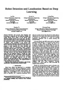
3. Experiments 3.1. Datasets The two publicly available datasets for our studies in this paper are: • Indiana Dataset [16]: Set consists of 7284 CXRs, both frontal and lateral images with disease annotations, such as cardiomegaly, pulmonary edema, opacity or pleural effusion. Indiana Set is collected from various hospitals affiliated with the Indiana University School of Medicine. The set is publicly available through Open-i SM, which is a multimodal (image + text) biomedical literature search engine developed by U.S. National Library of Medicine. A typical example of a normal CXR (left) and a CXR with cardiomegaly abnormality (right) is shown in Fig. 1. Visually, it can be observed that the heart in the cardiomegaly example is quite big compared to that of the normal CXR. • JSRT Dataset [17, 18]: Set compiled by the Japanese Society of Radiological Technology (JSRT). The set contains 247 chest X-rays, among which 154 have lung nodules (100 malignant cases, 54 benign cases), and 93 have no nodules. All X-ray images have a size of 2048 × 2048 pixels and a gray-scale color depth of 12 bit. The pixel spacing in vertical and horizontal directions is 0.175 mm. The JSRT set is publicly avail-

pathological sample, given as TPR = sensitivity =

TP TP + FN

(1)

TPR is also called sensitivity which is called such as this measure shows the degree to which does not miss a pathological sample. False positive rate (FPR) is proportion of normal samples that are incorrectly identified as pathological samples, given as, Figure 1. An example of Normal CXR (left) and an example of a cardiomegaly CXR (right) from Indiana dataset. The pathology in the right CXR can be easily distinguished from the abnormal size and shape of the heart.

able and has gold standard masks [18] for performance evaluation.

FPR = 1 − specificity =

FP FP + TN

(2)

The measure specificity shows the degree to which correctly identifies normal samples as normal. The objective of a classifier to attain high sensitivity as well as specificity so that the classifier attains low diagnosis error.

3.2. Deep Convolution Network Models

3.4. Localization Scheme

As described in section 2.1, deep convolutional networks (DCN) have achieved significantly higher accuracy than previous methods in disease detection in various diagnostic modalities. In many cases, these accuracies have surpassed human detection capabilities. Here, we explore the performance of various DCNs for heart disease detection on chest X-Rays. We use binary classification of Cardiomegaly and Pulmonary Atelectasis against normal chest X-Rays as representative examples. Results for other diseases are given in the supplementary materials. We explored several DCN models, e.g, AlexNet [2], VGG-Net [19] and ResNet [3]. These models vary in the number of convolution layers used and achieve higher classification accuracy as the number of convolution layers is increased. Specifically, ResNet and its variants have achieved superhuman performance on the celebrated ImageNet dataset.

The sensitivity of softmax score to occlusion of a certain region in the chest X-Ray was used to find which region in the image is responsible for the classification decision. We followed the localization using occlusion sensitivity described in [20]. In this experiment, a patch of square size is occluded in the CXRs and is observed whether the classifier can detect pathology in the presence of the occlusion. If the region corresponding pathology is occluded then the classifier should no longer detect the pathology with higher probability and thus this drop in probability indicates that the pathology is located at the location of the occlusion. This occluded region is slid through the whole CXR and thus a probability map of the pathology corresponding to the CXR is obtained. The regions where the probabilities are below a certain threshold indicates that the pathology is likely to be occupying that region. Thus, the pathology in the CXR can be localized.

3.3. Evaluation Metrics The quality of detection was evaluated in terms for four measures: accuracy, area under receiver operating characteristics (ROC) curve (AUC), sensitivity and specificity. The accuracy is the ratio of number of correctly classified samples to total samples. ROC curve is the graphical plot of true positive rate (TPR) vs false positive rate (FPR) of a binary classifier when classifier threshold is varied from 0 to 1. The number of pathological samples that are correctly identified as pathological sample by the classifier is called true positive (TP). The number of pathological samples that are incorrectly classified as normal by the classifier is called false negative (FN). The number of normal samples that are correctly classified as normal is called true negative (TN), and in a similar fashion, the number of normal samples that are incorrectly identified as pathological samples is called false positive (FP). True positive rate (TPR) is the proportion of pathological samples that are correctly identified as

4. Results 4.1. Classification 4.1.1

Classification using single models

Our first experiment use single model with DCNs finetuned from a model trained on ImageNet. Detection of cardiomegaly is done only for the frontal CXR images from the Indiana Dataset. It contains 250 frontal CXRs with cardiomegaly. In order to balance the binary classification, 250 normal frontal CXRs have been selected randomly from the database. Of these images, 200 of each class have been selected for training and 50 of each class for testing. In addition to training the DCNs, we also performed rule based features for cardiomegaly detection. Overall, we ran experiments with the following characteristics: (1) The NNs are fine-tuned on the Indiana dataset, (2) The NNs are finetuned using dropout technique [21], (3) The fusion of NN

Table 1. Experimenting on neural networks of different depths for Cardiomegaly detection.

A LEX N ET VGG-16 VGG-19 R ES N ET-50 R ES N ET-101 R ES N ET-152

ACCURACY (%) 86% 86% 92% 87% 92% 90%

AUC 0.9244 0.8720 0.9408 0.9330 0.9168 0.9056

S ENSITIVITY (%) 86% 96% 92% 94% 88% 92%

S PECIFICITY (%) 86% 76% 92% 80% 96% 88%

Table 2. Experimenting on neural networks of different depths for Cardiomegaly detection using dropout classifier.

A LEX N ET VGG-16 VGG-19 R ES N ET-50 R ES N ET-101 R ES N ET-152

ACCURACY (%) 88% 89% 88% 88% 87% 87%

AUC 0.9428 0.9024 0.8840 0.9045 0.9138 0.8772

feature and rule based features, and (4) The fusion of NN feature and rule based feature trained using dropout technique. The results are summarized in tables 1-2. In table 1, the results obtained by fine-tuning the DCNs are shown. We find that deeper models like VGG-19 and ResNet improve the classification accuracy significantly. For example, the accuracy of Cardiomegaly detection improves by 6 percentage point from that using AlexNet when VGG-16 and ResNet-101 are used. In order to understand the robustness of these results, we further calculate the sensitivity, specificity, sensitivity vs 1-specificity curve and derive the area under curve (AUC) metric for classification using different networks. We find that although ResNet-101 gives the highest specificity and VGG-16 gives the highest sensitivity, VGG-19 gives an overall better performance with the highest AUC of 0.94. The AUC calculated using VGG-19 is at least one percentage point higher than the other networks considered here. Adding dropout improves the classification accuracy of the shallower networks but degrades the performance of deep models. We find that VGG-16 and AlexNet achieve the highest accuracy and AUC respectively when dropout is used as shown in table 2. On the contrary, the accuracy of deeper models like ResNet-101 and VGG-19 drops by about 4 percentage points. For all these experiments, we found that taking features from earlier layers compared to later layers improve accuracy by 2 to 4 percentage points. Shallow DCN features are often useful for detecting small objects in images [22]. Our findings are similar for chest X-Ray abnormality classification as well. As an example, we are showing the performance obtained by taking features from different layers of ResNet-152 model. The candidate layers are chosen from the 4th, 5th and final stage of the network based on what

S ENSITIVITY (%) 88% 90% 86% 88% 82% 92%

S PECIFICITY (%) 88% 88% 90% 88% 92% 82%

Table 3. Candidate layers and their operation types chosen from ResNet-152 to test the features obtained from these layers.

L AYER NAME R E S 4 B 35 B R A N C H 2 C R E S 4 B 35 B R A N C H 2 C X R E S 4 B 35 R E S 4 B 35 X R E S5C B R A N C H2C R E S5C B R A N C H2C X R E S5C R E S5C X P O O L5

S TAGE 4 TH 4 TH 4 TH 4 TH 5 TH 5 TH 5 TH 5 TH F INAL

O PERATION C ONVOLUTION BATCH N ORMALIZATION R ESIDUAL C ONNECTION R E LU C ONVOLUTION BATCH N ORMALIZATION R ESIDUAL C ONNECTION R E LU AVERAGE P OLLING

type of operations they perform. The chosen layers and their corresponding operations are listed in Table 3. The notation of the layers is based on the pre-trained model obtained from MatConvNet Pre-train Library 1 . We trained five models to detect cardiomegaly using features from each of the layers and the average performance of these features in terms of accuracy, AUC, sensitivity, and specificity for Cardiomegaly detection are shown in Fig. 2. It can be observed that the performance of the final pooling layer (pool5) is degraded compared to the other layers in terms of accuracy, sensitivity and specificity. In particular features from residual connections (res4b35, res5c) and ReLU (res4b35x, res5cx) are considerably better with features from res4b35 providing highest accuracy. Similar observations are made for other ResNet variants, VGG nets and AlexNet. In addition to the DCN features, we experimented with DCN and rule based feature fusion for single model classi1 http://www.vlfeat.org/matconvnet/pretrained/

Accuracy AUC Sensitivity Specificity

92 90

Accuracy (%)

Average Metric (%)

94

88 86 84

90 85 80 75 70 65

Figure 2. Performance for features extracted from different layers of ResNet-152 for Cardiomegaly detection. Features from earlier layers provides much better accuracy than the final pooling layer (pool5) with highest from resb35 features.

fication. The rule based features that were used in the study are 2D-cardio-thoracic ratio (CTR) and cardio-thoracic area ratio (CTAR) [5]. The 2D-CTR is the ratio between the perimeter of the heart region to the perimeter of the entire thoracic region and formulated as 2D-CTR =

Perimeter of Heart Perimeter of Thoracic Region

(3)

while CTAR, the ratio between area of the heart region to the sum of the area of the left and right lung region, is formulated as CTAR =

Area of Heart . (4) Area of Left Lung + Area of Right Lung

In the experiments involving rule based features, we concatenated the features with the features extracted from a DCN and trained a fully connected layer to detect cardiomegaly. However, the results degraded and hence are not shown here. Observation from these single model classification results is that different figure of merit is maximized by different DCNs. We wanted to explore if this is expected or due to some limitation of the data or training process itself. Hence, rather than taking a single train-test split of the data, we randomly split the train-test data and trained nine different model for each architecture. Then we calculated the mean and standard deviation for the figure of merits of interest. The results can be seen in table 4. We find that after averaging the nine random train-test sample results, a clear trend emerges where a single model, ResNet-152 in this case, achieves the highest accuracy, AUC and sensitivity. The mean specificity for ResNet-152, in this case is close to the highest number, however, the max specificity is indeed highest for ResNet-152.

Area Under Curve

res

4b 3 res 5_bra 4b nc 35 h2 _b c ran ch2 cx res 4b 3 r 5 res es4b 5c_ 35 bra x nch 2cx res 5c res 5cx po ol5

82

0

50

0

50

100

150

200

250

100

150

200

250

Training Size/Class

0.90 0.85 0.80 0.75 0.70

Training Size/Class

Figure 3. Accuracy (top) and AUC (bottom) of Cardiomegaly detection as number of samples in training set is increased. Both metrics increase as training size is increased.

Having around 600 images for training a network is not sufficient. We wanted to see how does the mean accuracy and the standard deviation vary as we change the number of training examples. Since averaging over multiple train-test splits gave a robust classification accuracy and other figures of merit, we used this classification process to identify the deviation of the result as a function of the number of training images. The results are shown in Fig. 3. As expected, for both accuracy and AUC, the mean is lower and deviation is higher for less than 50 training example per category. As the number of example increases, the mean increases and the deviation decreases coming to a saturation at about 200 images. In order to check if the same model gives the highest accuracy for different abnormalities, we model pulmonary atelectasis using the same averaging process described above. Our dataset for the detection of pulmonary atelectasis contains available 312 frontal CXR images with pulmonary atelectasis and randomly chosen 312 normal frontal CXRs from the Indiana Dataset. We partitioned the dataset in train and test set such that 232 of each class have been selected for training and 80 of each class for testing. We have run our program with 15 different seeds and reported the overall performance metrics in the table 5 as (mean ± s.d.). We find that whereas ResNet-152 gave the highest accuracy

Table 4. Experimenting on neural networks of different depths for Cardiomegaly detection.

A LEX N ET VGG-16 VGG-19 R ES N ET-50 R ES N ET-101 R ES N ET-152

ACCURACY (%) 84.73 ± 3.03% 87.37 ± 1.76% 87.97 ± 2.04% 87.33 ± 1.96% 86.30 ± 2.00% 88.03 ± 2.27%

AUC 0.91 ± 0.03 0.91 ± 0.02 0.91 ± 0.02 0.91 ± 0.02 0.91 ± 0.02 0.92 ± 0.02

S ENSITIVITY (%) 85.53 ± 4.75% 87.20 ± 3.00% 88.60 ± 2.26% 86.87 ± 3.76% 88.60 ± 2.26% 88.87 ± 5.77%

S PECIFICITY (%) 83.93 ± 3.15% 87.53 ± 2.07% 87.33 ± 3.72% 87.80 ± 3.75% 87.33 ± 3.72% 87.20 ± 4.55%

Table 5. Experimenting on neural networks of different depths for Pulmonary Atlectasis detection.

A LEX N ET VGG-16 VGG-19 R ES N ET-50 R ES N ET-101 R ES N ET-152

ACCURACY (%) 76.25 ± 2.66% 79.54 ± 2.75% 80.33 ± 2.10% 82.17 ± 2.25% 81.17 ± 2.62% 80.29 ± 2.03%

AUC 0.81 ± 0.02 0.84 ± 0.03 0.84 ± 0.03 0.86 ± 0.02 0.86 ± 0.02 0.85 ± 0.02

for cardiomegaly detection, for pulmonary atelectasis detection ResNet-50 gives the highest accuracy and other figures of merit. Only ResNet-101 have a slightly higher specificity. This shows that there is no single model appropriate for all abnormalities, rather the suitable network varies for different abnormalities. This observation is consistent with the conclusions drawn in [23]. In this case, ResNet-152 which gave the highest accuracy for cardiomegaly detection achieves almost two percentage point reduced accuracy compared to ResNet-50 which is a significant deviation. 4.1.2

Classification using ensemble of models

We trained four different instances of each of the DCNs, i.e, AlexNet, VGG-16, VGG-19, ResNet-50, ResNet-101 and ResNet-152, to detect cardiomegaly. Thus a total of 24 networks were trained on the same training data. There are a number of ways to perform ensemble on the trained model. The methods include linear averaging, bagging, boosting, stacked regression [24] etc. Since, the number of images in the training dataset is only 460, which is far less than the number of trainable parameters in the classifiers, the individual classifiers always overfit the training set. In this situation, if bagging, boosting and/or stacked regression are employed to build the ensemble model, it will result in a completely biased model. Thus, the ensemble models were obtained by using simple linear averaging of the probabilities given by the individual models. The performance of the ensembles was measured using 50 cardiomegaly and 50 normal images for all the possible combinations of the trained individual models. The performance of these combinations is shown in Fig. 4 using boxplots. The horizontal red bars indicate the 50 percentile values and the spread of the blue boxes indicate the 25 and 75 percentile values.

S ENSITIVITY (%) 76.17 ± 4.42% 77.25 ± 6.43% 79.92 ± 5.76% 81.58 ± 5.33% 79.42 ± 5.76% 78.08 ± 6.99%

S PECIFICITY (%) 76.33 ± 6.49% 81.83 ± 6.84% 80.75 ± 6.10% 82.75 ± 3.64% 82.92 ± 5.32% 82.50 ± 4.15%

The black stars indicate extreme points in the data. It can be observed from the figure that, combinations of 7 to 10 models can achieve higher accuracy, however they have the largest spread. On the other hand, as number of models in the ensemble increases, the accuracy of the ensemble model converges to a certain value which for this experiment was 92%. The ROC curves of one instance AlexNet, VGG-19, ResNet-152 and one ensemble model, that is linear average of 6 different types of DCNs, are shown in Fig. 5. The curves are obtained using 50 cardiomegaly and 50 normal images. The AUC obtained for each model are 0.8624, 0.8888, 0.8896 and 0.9728, respectively. We can understand from the AUC values that, the separation between the pathology class and the normal class increases when an ensemble of multiple DCNs are performed. For the ensemble model to be used as a screening tool with high sensitivity, the operating point on the curve is set to achieve 98% sensitivity. The specificity obtained at this point is 82%. The second operating point is set for high specificity of 98% and the sensitivity at this point is 86%.

4.2. Localization For any diagnostic task, it is desirable to gain intuitive understanding of why a certain classification decision is made rather than being a black box method. In other words, it is desirable to distinguish features that contributed most to certain abnormality in the entire chest X-Ray. There are various ways of achieving this goal [20, 25–27]. The method used in [20] is the simplest, where a patch is occluded in the image to measure its impact on the eventual classification confidence score. We have used this method to find the regions in the image responsible for a certain abnormality detection. As a representative example, we have used car-

0.98 0.96

Accuracy

0.94 0.92 0.90 0.88 0.86 0.84

1 2 3 4 5 6 7 8 9 10 11 12 13 14 15 16 17 18 19 20 21 22 23 24

0.82

Number of Models in Ensemble

Figure 4. Ensemble of all the combinations of the trained models using linear averaging. As the number of models in the ensemble increases the performance become robust.

4.2.1

TPR or Sensitivity

1.0 0.8 0.6 0.4 AlexNet (area = 0.8624) VGG-19 (area = 0.888) ResNet-152 (area = 0.8896) Ensemble (area = 0.9728)

0.2 0.0

0.0

0.2

0.4

0.6

FPR or (1-Specificity)

0.8

1.0

Figure 5. ROC Curve of AlexNet, VGG-19, ResNet-152 and an ensemble model. The ensemble model shows increased area under the curve compared to individual models.

diomegaly and pulmonary edema which occur in heart and lung areas respectively. The localization scheme described in section 3.4 is followed with a patch size of 40 × 40 pixels taking lowest 20% values of probabilities. Instead of gray level occlusion as in [20] we found that black level occlusion works better for CXRs. This is due to the fact that the CXRs themselves are mostly gray level and occlusion of the same level does not hide much information compared to the neighborhood.

Cardiomegaly Localization

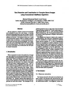
The localization of abnormalities in cardiomegaly examples are shown in Fig. 6. Here, 20% of the image area is shown which has the highest sensitivity. It can be observed from the figures that the network is indeed most sensitive to the region where the heart is larger than a normal heart. We have performed this experiment on 50 cardiomegaly and 50 normal images and found this localization to be consistent for most examples. There is not much functional difference between a normal and cardiomegaly example other than the fact that the heart in cardiomegaly is larger than a normal heart. Given the fact that the normal images could also have various size of heart depending on the age or physical attributes of a patient, we found this level of localization sensitivity to be remarkable. Also interesting is the fact that the standard rule based features like CTR and CTAR take into account the relative size of heart and lung to determine if there is cardiomegaly present or not. In the DCN localization experiment, we see counter-intuitively that most of the signals contributing to the softmax score are coming from the heart only. This means that there are characteristic features in the shape of the heart and its surrounding regions that alone is sufficient to detect cardiomegaly. The lung and its relative size are probably lesser important features when trying to detect cardiomegaly. This observation is counterintuitive and needs to be explored further in future work.

(a)

(b)

Figure 6. The localization observed for Cardiomegaly. The localized area by the probability map is superimposed on the CXRs and localization around the heart is observed. This observation is counter intuitive to the rule based method which involves relative size of heart and lung.

an accuracy of 73.9%. The results have a slight variation due to the random choice of normal and cardiomegaly images. However, it is evident that all DCN based approaches outperform the rule based method. As stated earlier, DCNs were fine tuned on a sample of 560 images and validated on 100 images. Among the independent DCN models, VGG19 model achieves the highest accuracy of 92% and highest AUC of 0.9408 for detecting cardiomegaly. The ensemble model, which is linear average of the six individual DCN models, shows the best accuracy of 93% and AUC of 0.9728. The accuracy is 17% point higher than the rule based system and the AUC is 3% point higher than the nearest VGG-19 model. A brief discussion about the rule based approach is given in the supplementary materials section.

5. Conclusion

(a)

(b)

Figure 7. The localization observed for pulmonary edema. The localized area by the probability map is superimposed on the CXRs and localization around excess fluid in lungs is observed.

4.2.2

Pulmonary Edema Localization

In order to test the effectiveness of the localization procedure in areas other than the heart region, we chose pulmonary edema which occurs in the lung region. Also, pulmonary edema is detected by the net like white structure in the lung area. No anatomical shape change is associated with the abnormality. We have found that the localization is obtained best when the ROIs of lungs are taken to compute the map. Following the scheme in section 3.4, localization experiment on pulmonary edema is performed as shown in Fig. 7. The features tend to localize around the excess fluid in the lungs. We found that this procedure is not able to localize fine features like septal or Kerley B lines. Sometimes it localizes areas outside the lungs region. For Fig. 7(a), this occurs due to the fact that ROI includes these regions.

4.3. Comparison between Rule based and DCN based cardiomegaly detection A comparison between rule based and DCN based cardiomegaly detection is shown in table 6. State-of-the-art method [5] achieves an accuracy of 76.5% while classifying between 250 cardiomegaly and 250 normal images. In verifying that claim, we reproduced those results and achieved

In summary, we have explored various DCNN for chest X-Ray abnormality detection and localization. We have found the existing literature to be insufficient for making comparison of various machine learning techniques either due to studies reported on private datasets or not reporting the test scores in proper detail. In order to overcome these difficulties, we have used a publicly available chest X-Ray dataset and studied the performance of known DCN architectures on different abnormalities. We find that the same DCN architecture doesn’t perform well across all abnormalities. Also, for this dataset, a consistent detection result emerges when multiple random train/test split is performed and their average is used as the accuracy measure. Shallow features or earlier layers consistently provide higher detection accuracy compared to deep features. We have also found ensemble models to improve classification significantly compared to single model. Our experiments of incorporating DCN features with rule based features degraded the accuracy. Combining these insights, we have reported the highest accuracy on chest X-Ray abnormality detection. For the cardiomegaly classification task, where we could make a comparison with rule based methods, the deep learning method improves the accuracy by a staggering 17 percentage point. We have also performed localization of features responsible for classification decision. We found that for spatially spread out abnormalities like cardiomegaly and pulmonary edema, the network can localize the abnormalities successfully most of the time. However, the localization fails for pointed features like lung nodule or bone fracture. One remarkable result of the cardiomegaly localization is that the heart and its surrounding region is most responsible for cardiomegaly detection. This is counterintuitive compared to rule based models where the ratio of heart and lung area is used as a measure for cardiomegaly. We believe that through deep learning based classification and localization, we will discover many more interesting features that are not considered traditionally.

Table 6. Comparison between Rule-based and DCN based approaches for Cardiomegaly detection.

C ANDEMIR RULE BASED FEATURES A LEX N ET VGG-16 VGG-19 R ES N ET-50 R ES N ET-101 R ES N ET-152 E NSEMBLE

ACCURACY (%) 76.5% 73.9% 86% 86% 92% 87% 92% 90% 93%

While finishing this paper, we became aware of a new dataset announcement and paper focused on similar problem [28]. It would be interesting to apply the techniques discussed in this paper on this new dataset in the future.

6. Acknowledgement This research used resources of the National Energy Research Scientific Computing Center, a DOE Office of Science User Facility supported by the Office of Science of the U.S. Department of Energy under Contract No. DE-AC0205CH11231. Thanks Leonid Oliker at NERSC for sharing his allocation on the OLCF Titan supercomputer with us on project CSC103. Thanks to Hoo-Chang Shin for correspondence regarding the Indiana chest X-Ray dataset.

AUC − − 0.9244 0.8720 0.9408 0.9330 0.9168 0.9056 0.9728

S ENSITIVITY (%) 77.1% 79.8% 86% 96% 92% 94% 88% 92% 94%

S PECIFICITY (%) 76.4% 68% 86% 76% 92% 80% 96% 88% 92%

Medical Imaging. International Society for Optics and Photonics, 2016, pp. 978 517–978 517. [6] S. Candemir, S. Jaeger, K. Palaniappan, J. P. Musco, R. K. Singh, Z. Xue, A. Karargyris, S. Antani, G. Thoma, and C. J. McDonald, “Lung segmentation in chest radiographs using anatomical atlases with nonrigid registration,” IEEE transactions on medical imaging, vol. 33, no. 2, pp. 577–590, 2014. [7] S. Jaeger, A. Karargyris, S. Candemir, L. Folio, J. Siegelman, F. Callaghan, Z. Xue, K. Palaniappan, R. K. Singh, S. Antani et al., “Automatic tuberculosis screening using chest radiographs,” IEEE transactions on medical imaging, vol. 33, no. 2, pp. 233–245, 2014.

[1] P. Campadelli and E. Casiraghi, “Lung field segmentation in digital postero-anterior chest radiographs,” in International Conference on Pattern Recognition and Image Analysis. Springer, 2005, pp. 736–745.

[8] A. Kumar, Y.-Y. Wang, K.-C. Liu, I.-C. Tsai, C.C. Huang, and N. Hung, “Distinguishing normal and pulmonary edema chest x-ray using gabor filter and svm,” in Bioelectronics and Bioinformatics (ISBB), 2014 IEEE International Symposium on. IEEE, 2014, pp. 1–4.

[2] A. Krizhevsky, I. Sutskever, and G. E. Hinton, “Imagenet classification with deep convolutional neural networks,” in Advances in Neural Information Processing Systems, 2012, pp. 1097–1105.

[9] M. R. Zare, A. Mueen, M. Awedh, and W. C. Seng, “Automatic classification of medical x-ray images: hybrid generative-discriminative approach,” IET Image Processing, vol. 7, no. 5, pp. 523–532, 2013.

[3] K. He, X. Zhang, S. Ren, and J. Sun, “Deep residual learning for image recognition,” in Proceedings of the IEEE Conference on Computer Vision and Pattern Recognition, 2016, pp. 770–778.

[10] H.-C. Shin, K. Roberts, L. Lu, D. Demner-Fushman, J. Yao, and R. M. Summers, “Learning to read chest x-rays: recurrent neural cascade model for automated image annotation,” in Proceedings of the IEEE Conference on Computer Vision and Pattern Recognition, 2016, pp. 2497–2506.

References

[4] J. M. Carrillo-de Gea, G. Garc´ıa-Mateos, J. L. Fern´andez-Alem´an, and J. L. Hern´andez-Hern´andez, “A computer-aided detection system for digital chest radiographs,” Journal of Healthcare Engineering, vol. 2016, 2016. [5] S. Candemir, S. Jaeger, W. Lin, Z. Xue, S. Antani, and G. Thoma, “Automatic heart localization and radiographic index computation in chest x-rays,” in SPIE

[11] Y. Bar, I. Diamant, L. Wolf, S. Lieberman, E. Konen, and H. Greenspan, “Chest pathology detection using deep learning with non-medical training,” in Biomedical Imaging (ISBI), 2015 IEEE 12th International Symposium on. IEEE, 2015, pp. 294–297. [12] G. Litjens, T. Kooi, B. E. Bejnordi, A. A. A. Setio, F. Ciompi, M. Ghafoorian, J. A. van der Laak,

B. van Ginneken, and C. I. S´anchez, “A survey on deep learning in medical image analysis,” arXiv preprint arXiv:1702.05747, 2017. [13] D. Wang, A. Khosla, R. Gargeya, H. Irshad, and A. H. Beck, “Deep learning for identifying metastatic breast cancer,” arXiv preprint arXiv:1606.05718, 2016. [14] V. Gulshan, L. Peng, M. Coram, M. C. Stumpe, D. Wu, A. Narayanaswamy, S. Venugopalan, K. Widner, T. Madams, J. Cuadros et al., “Development and validation of a deep learning algorithm for detection of diabetic retinopathy in retinal fundus photographs,” JAMA, vol. 316, no. 22, pp. 2402–2410, 2016.

[22] K. Ashraf, B. Wu, F. Iandola, M. Moskewicz, and K. Keutzer, “Shallow networks for high-accuracy road object-detection,” in Proceedings of the 3rd International Conference on Vehicle Technology and Intelligent Transport Systems, 2017, pp. 33–40. [23] H. Azizpour, A. Sharif Razavian, J. Sullivan, A. Maki, and S. Carlsson, “From generic to specific deep representations for visual recognition,” in Proceedings of the IEEE Conference on Computer Vision and Pattern Recognition Workshops, 2015, pp. 36–45. [24] L. Breiman, “Stacked regressions,” Machine learning, vol. 24, no. 1, pp. 49–64, 1996.

[15] A. Esteva, B. Kuprel, R. A. Novoa, J. Ko, S. M. Swetter, H. M. Blau, and S. Thrun, “Dermatologistlevel classification of skin cancer with deep neural networks,” Nature, vol. 542, no. 7639, pp. 115–118, 2017.

[25] S. Bach, A. Binder, G. Montavon, F. Klauschen, K.R. M¨uller, and W. Samek, “On pixel-wise explanations for non-linear classifier decisions by layer-wise relevance propagation,” PloS one, vol. 10, no. 7, p. e0130140, 2015.

[16] D. Demner-Fushman, M. D. Kohli, M. B. Rosenman, S. E. Shooshan, L. Rodriguez, S. Antani, G. R. Thoma, and C. J. McDonald, “Preparing a collection of radiology examinations for distribution and retrieval,” Journal of the American Medical Informatics Association, vol. 23, no. 2, pp. 304–310, 2016.

[26] J. T. Springenberg, A. Dosovitskiy, T. Brox, and M. Riedmiller, “Striving for simplicity: The all convolutional net,” arXiv preprint arXiv:1412.6806, 2014.

[17] J. Shiraishi, S. Katsuragawa, J. Ikezoe, T. Matsumoto, T. Kobayashi, K.-i. Komatsu, M. Matsui, H. Fujita, Y. Kodera, and K. Doi, “Development of a digital image database for chest radiographs with and without a lung nodule: receiver operating characteristic analysis of radiologists’ detection of pulmonary nodules,” American Journal of Roentgenology, vol. 174, no. 1, pp. 71–74, 2000. [18] B. Van Ginneken, M. B. Stegmann, and M. Loog, “Segmentation of anatomical structures in chest radiographs using supervised methods: a comparative study on a public database,” Medical image analysis, vol. 10, no. 1, pp. 19–40, 2006. [19] K. Simonyan and A. Zisserman, “Very deep convolutional networks for large-scale image recognition,” CoRR, vol. abs/1409.1556, 2014. [20] M. D. Zeiler and R. Fergus, “Visualizing and understanding convolutional networks,” in European conference on computer vision. Springer, 2014, pp. 818– 833. [21] N. Srivastava, G. E. Hinton, A. Krizhevsky, I. Sutskever, and R. Salakhutdinov, “Dropout: a simple way to prevent neural networks from overfitting.” Journal of Machine Learning Research, vol. 15, no. 1, pp. 1929–1958, 2014.

[27] B. Zhou, A. Khosla, A. Lapedriza, A. Oliva, and A. Torralba, “Learning deep features for discriminative localization,” in Proceedings of the IEEE Conference on Computer Vision and Pattern Recognition, 2016, pp. 2921–2929. [28] X. Wang, Y. Peng, L. Lu, Z. Lu, M. Bagheri, and R. M. Summers, “Chestx-ray8: Hospital-scale chest x-ray database and benchmarks on weakly-supervised classification and localization of common thorax diseases,” arXiv preprint arXiv:1705.02315v2, 2017.

7. Supplementary Materials 7.1. Rule based Approach in Detecting Cardiomegaly

Radon transform R at 0 degree

7.1.1

Using Radon Transform and Bhattacharyya Distance to find visually similar images

5

×105 Sample Image Most Similar Image Least Similar Image

4

(b)

(c)

(d)

3 2 1 0

−500

0

500

Radial Coordinates for 0 degree

Figure 8. Comparison of Radon Transforms among sample CXR, the most similar and the least similar CXR at 0 Degree

The method uses existing CXRs and their radiologist marked lung/heart boundaries as models, and estimates the lung/heart boundary of a patient X-ray by registering the model X-rays to the patient X-ray. We use a public CXR dataset (JSRT) with reference boundaries. The radon function computes projections of an image matrix along specified directions. To represent an image, the radon function takes multiple, parallel-beam projections of the image from different angles by rotating the source around the center of the image. We transformed the image from 0 to 90 degrees, at 15 degrees interval, and calculated Bhattacharya distance between radon transform of test CXR and sample CXRs to find 5 visually similar samples. The most similar X-rays will register to the patients X-ray in the next stage. The main purpose of measuring the similarity is to increase the correspondence performance and decrease the computational expense during registration. 7.1.2

(a)

Calculating correspondence between test CXR and model CXRs using SIFTFlow

After the model selection, we compute the correspondence map between the model X-ray and patient X-ray. The correspondence map computation is conducted by modeling the patient X-ray with local image features, and matching the most similar locations. For the correspondence map computation, we employ the SIFT-flow algorithm. The computed map is considered to be a transformation from model X-rays to the patient X-ray. The transformation

Figure 9. (a) Test CXR, (b) Sample Similar CXR, (c) Sample CXR’s lung and heart model atlas, (d) Localized heart and lung in test CXR.

matrix is applied to the model masks to transform them into the approximate lung/heart model for the patient X-ray.

7.1.3

Rule based feature extraction

Rule based features were extracted using 3 and 4 and SVM was used to classify between cardiomegaly and normal CXR images.

7.2. Classification Results on the 20 chest X-Ray abnormalities In this section, we report the classification accuracy, sensitivity and specificity using the ResNet-152 model. We hope that these numbers will set a benchmark to compare against other machine learning methods on this dataset.

Table 7. Performance analysis of detecting 20 abnormalities in CXR with ResNet-152. A BNORMALITIES C ALCIFIED G RANULOMA C ALCINOSIS G RANULOMATOUS D ISEASE P LEURAL E FFUSION ATHEROSCLEROSIS A IRSPACE D ISEASE N ODULE P ULMONARY E MPHYSEMA S COLIOSIS F RACTURES B ONE O STEOPHYTE P ULMONARY C ONGESTION B ULLOUS E MPHYSEMA S UBCUTANEOUS E MPHYSEMA S PONDYLOSIS E MPHYSEMA G RANULOMA H ERNIA H IATAL P ULMONARY D ISEASE C HRONIC O BSTRUCTIVE P ULMONARY E DEMA

ACCURACY (%) 64.74% 68.39% 68.37% 85.56% 79.49% 79.41% 67.19% 91.94% 77.59% 79.63% 73.81% 95.24% 82.50% 87.50% 67.50% 86.84% 68.75% 89.29% 85.71% 89.29%

AUC 0.65 0.79 0.71 0.89 0.84 0.78 0.69 0.96 0.83 0.78 0.76 0.97 0.87 0.91 0.65 0.94 0.66 0.90 0.87 0.91

S ENSITIVITY (%) 61.05% 45.98% 61.22% 86.67% 82.05% 94.12% 46.88% 93.55% 68.97% 88.89% 85.71% 100.00% 75.00% 85.00% 80.00% 84.21% 93.75% 92.86% 92.86% 92.86%

S PECIFICITY (%) 68.42% 90.80% 75.51% 84.44% 76.92% 64.71% 87.50% 90.32% 86.21% 70.37% 61.90% 90.48% 90.00% 90.00% 55.00% 89.47% 43.75% 85.71% 78.57% 85.71%