Accelerated Model Checking of Parametric Markov Chains - Computer ...

Accelerated Model Checking of Parametric Markov Chains Paul Gainer, Ernst Moritz Hahn, and Sven Schewe University of Liverpool, UK {p.gainer,e.m.hahn,sven.schewe}@liverpool.ac.uk

Abstract. Parametric Markov chains occur quite naturally in various applications: they can be used for a conservative analysis of probabilistic systems (no matter how the parameter is chosen, the system works to specification); they can be used to find optimal settings for a parameter; they can be used to visualise the influence of system parameters; and they can be used to make it easy to adjust the analysis for the case that parameters change. Unfortunately, these advancements come at a cost: parametric model checking is—or rather was—painstakingly slow. To make the analysis of parametric Markov models scale, we need three ingredients: clever algorithms, the right data structure, and good engineering. Clever algorithms are often the main (or sole) selling point; and we face the trouble that this paper focuses on the latter ingredients to efficient model checking. Consequently, our easiest claim to fame is in the speed-up we have realised: around 1.5 to 2 orders of magnitude.

1

Introduction

The analysis of parametric Markov models is a young and growing field of research. As not only the research direction but also the term ‘parametric Markov models’ is attractive, it has been used for various generalisations of traditional Markov models. We use Markov chains, where the parameter is used to determine the probabilities and rewards, such that we can reason about the likelihood of obtaining simple temporal properties like safety and reachability as well as standard reward functions, such as long-run average. What we do not intend to do in this paper is to use parameters to change the size of the system or the shape of the Markov chain. (The latter can, of course, be encoded by using parameters to assign a probability of 0 to an edge, effectively removing it. This would, however, come at the cost of efficiency and is not what we want to use the parameters for.) Using parameters to describe the probabilities of transitions is not quite as easy as it sounds: even when parameters appear in a simple way, like ‘p’ or ‘1 − p’, the terms that represent the likelihood of obtaining a temporal property or an expected reward can quickly become quite intricate. One ends up with rational functions. We make a virtue of necessity by using this as a motivation to allow for using rational functions of the occurring parameters to represent the probabilities and payoffs.

To allow for an efficient analysis of such complex parametrised systems, we have taken a look at different strategies for the evaluations of—parametric and non-parametric—Markov chains, and considered their suitability for our purposed. We found the stepwise elimination of vertices from a model to be the most attractive approach to port. Broadly speaking, this approach works like the transformation from finite automata to regular expressions: a vertex is removed, and the new structure has all successors of this state as—potentially new—successors of the predecessors of this vertex. In the transformation from finite automata to regular expressions, one changes the expressions on the edges, while we adjust the probabilities and, if applicable, the rewards on the edges. When using this approach with explicit probabilities and rewards, one ends up with a DAG structure in the evaluation. This DAG structure has been exploited to reduce the cost of re-calculating the probabilities for simple temporal properties or expected rewards, and it proves that it also integrates nicely into our framework, where the probabilities and rewards are provided as rational functions. In fact it integrates so naturally that it seems surprising in hindsight that it has not been discovered earlier. The natural connection occurs when choosing a similar data structure to represent the rational functions that represent the probabilities and rewards. To make full use of the DAG structure that comes with the elimination, we represent these functions in the form of arithmetic circuits—which are essentially DAGs. We have integrated the resulting representation organically in a small extension of ePMC, and tested it on a range of case studies. We have obtaine a speed-up of a hefty factor of 20 to 120 when compared to storing functions in terms of coprime numerator and denominator polynomials. Related work. For (discrete-time) Markov chains (MCs), Daws [6] has devised a language-theoretic approach to solve this problem. In this approach, the transition probabilities are considered as letters of an alphabet. Thus, the model can be viewed as a finite automaton. Then, based on the state elimination method [22], a regular expression that describes the language of such an automaton is calculated. In a post-processing step, this regular expression is recursively evaluated, resulting in a rational function over the parameters of the model. One of the authors has been involved in extending and tuning this method [16] so as to operate with rational functions, which are stored as coprime numerator and denominator polynomials rather than with regular expressions. The process of computing a function that describes properties (like reachability probabilities or long-run average rewards) that depend on model parameters is often costly. However, once the function has been obtained, it can very efficiently be evaluated for given parameter instantiations. Because of this, parametric model checking of Markov models has also attracted attention in the area of runtime verification, where the acceptable time to obtain values is limited [3,11]. Other works in the area are centred around deciding the validity of boolean formulas depending on the parameter range using SMT solvers or extending these techniques to models that involve nondeterminism [7,14,5,27]. 2

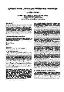
1−x As an example for a parax 3 metric model, consider Figure 1. Knuth and Yao [24] x x have shown how a six-sided 1 dice can be simulated by rex 1−x 4 peatedly tossing a coin. The 1−x idea is to build a Markov 0 chain with transition probx x 1−x 5 abilities of only 0.5 or 1. 2 Borrowing a model from the 1−x 1−x PRISM website, we have extended this example to a bi6 1−x ased dice, simulated by tossx ing a biased coin. With probability x we see heads, while with probability 1 − x we see Fig. 1: Simulating a biased dice by a biased coin. tails. This way, we move around in the Markov chain until we obtain a result. Organisation of the paper. After formalising our setting in Section 2, we describe how we exploit DAGs in the representation of rational functions, and exploit them using synergies with the DAG-style state elimination technique, in Section 3. We then describe how to expand this technique to determine long-run average rewards in Section 4. In Section 5, we evaluate our approach on a range of benchmarks, and discuss the results briefly in Section 6.

2 2.1

Preliminaries Parametric Markov chains with state rewards

Let V = {v1 , . . . , vn } denote a set of variables over R. A polynomial g over V is a sum of monomials X g(v1 , . . . , vn ) = ai1 , . . . ,in v1i1 . . . vnin , i1 ,...,in

where each ij ∈ N and each ai1 , . . . ,in ∈ R. A rational function f over a set of 1 ,...,vn ) variables V is a fraction f (v1 , . . . , vn ) = ff21 (v (v1 ,...,vn ) of two polynomials f1 , f2 over V . We denote the set of rational functions from V to R by FV . Definition 1. A parametric Markov chain (PMC) is a tuple D = (S, s, P, V ), where S is a finite set of states, s is the initial state, V = {v1 , . . . , vn } is a finite set of parameters, and P is the probability matrix P : S × S → FV . A path ω of a PMC D = (S, s, P, V ) is a non-empty finite, or infinite, sequence s0 , s1 , s2 , . . . where si ∈ S and P(si , si+1 ) > 0 for i > 0. We let Ω denote the set of infinite paths. With Prs , we denote the parametric probability measure over Ω assuming that we start in state s, with Pr = Prs . We use Exps , Exp to 3

Algorithm 1 Parametric Reachability Probability for PMCs 1: procedure StateElimination(D, B) 2: requires: A PMC D = (S, s, P, V ) and set of target states B ⊆ S, where reachD (s, s) holds for all s ∈ S. 3: E←S 4: while E 6= ∅ do 5: se ← choose(E) 6: E ← E \ {se } 7: for all s ∈ postD (se ) do 8: P(se , s) ← P(se , s)/(1 − P(se , se )) 9: end for 10: P(se , se ) ← 0 11: for all (s1 , s2 ) ∈ preD (se ) × postD (se ) do 12: P(s1 , s2 ) ← P(s1 , s2 ) + P(s1 , se )P(se , s2 ) 13: end for 14: if se 6= s ∧ se ∈ / B ∧ postD (se ) 6= ∅ then 15: Eliminate(D, se ) // remove se and incident transitions from D 16: end if 17: end while P 18: return s∈B P(s, s) 19: end procedure

denote according expectations. With X(D)s,i : Ω → S, X(D)s,i (s0 , s1 , . . .) = si we denote the random variable expressing the state occupied at step i ≥ 0, and let X(D)i = X(D)s,i . Definition 2. Given a PMC D = (S, s, P, V ), the underlying graph of D is given by GD = (S, E) where E = {(s, s0 ) | P(s, s0 ) > 0}. A bottom strongly connected component (BSCC) is a set A ⊆ S such that in the underlying graph each state s1 ∈ A can reach each state s2 ∈ A and there is no s3 ∈ S \A reachable from s1 . Given a state s, we denote the set of all immediate predecessors and successors of s in the underlying graph of D by preD (s) and postD (s), respectively, excluding s itself. We write reachD (s, s0 ) if s0 is reachable from s in the underlying graph of D. Given a PMC D = (S, s, P, V ) we are interested in computing the function that represents the probability of reaching some set of target states B ⊂ S. Reach(D, B) = Pr [∃i ≥ 0.X(D)s,i ∈ B] Our base algorithm to obtain this value is described in Algorithm 1. A state se ∈ S is selected, and then eliminated by considering each pair (s1 , s2 ) ∈ preD (se ) × postD (se ) and updating the existing probability P(s1 , s2 ) by the probability of reaching s2 from s1 via se . Heuristics to determine the order in which states are chosen for elimination by the choose function are discussed in Section 5.5. 4

Definition 3. A parametric reward function for a PMC D = (S, s, P, V ) is a function r : S → FV . The reward function labels states in D with a rational function over V that corresponds to the reward that is gained if that state is visited. Given a PMC D = (S, s, P, V ) and a reward function r : S → FV , we are interested in the parametric expected accumulated reward defined as "∞ # X Acc(D, r) = Exp r(X(D))s,i i=0

or a variation [25], the parametric expected accumulated reachability reward given B ⊆ S defined as   {j|X(D)s,j ∈B} X r(X(D))s,i  . Acc(D, r, B) = Exp  i=0

This can, however, be transformed to the former. Algorithm 1 can be extended to compute the parametric expected accumulated reward. In addition to updating the probability matrix for each predecessor and successor pair, we also update the reward function as follows: r(s1 ) ← r(s1 ) + P(s1 , se )

P(se , se ) r(se ). 1 − P(se , se )

The updated value for r(s1 ) reflects the reward that would be accumulated if a transition would be taken from s1 to se , where the expected number of self-loops P(se ,se ) would be 1−P(s . Upon termination, the algorithm returns the value r(s). e ,se )

3

Representing Formulas using Directed Acyclic Graphs

In existing tools for parametric model checking of Markov models, rational func1 ,...,vn ) tions have traditionally been represented in the form f (v1 , . . . , vn ) = ff12 (v (v1 ,...,vn ) , where f1 (v1 , . . . , vn ) and f2 (v1 , . . . , vn ) [15,8,26] are coprime. As a result, for some cases the representations of such functions are very short. Often, during the state elimination phase, large common factors can be cancelled out, such that one can operate with relatively small functions throughout the whole algorithm. There are, however, many cases without—or with very few—large common factors. The nominator-denominator representations then become larger and larger during the analysis. In this case, the analysis is slowed down severely, mostly by the time taken for the cancellation of common factors. Cancelling out such factors is non-trivial, and indeed a research area in itself. In addition, if formulas become large, this can also lead to out-of-memory problems. To overcome this issue, we propose the representation of rational functions by arithmetic circuits. These arithmetic circuits are directed acyclic graphs (DAG). 5

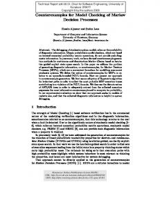
Terminal nodes are labelled with either a variable of the set of parameters V , or with a rational number. Non-final nodes are labelled with a function to be applied on the nodes it has edges to. In our setting, we require two unary functions, additive inverse and multiplicative inverse, and two binary functions, addition and multiplication. All functions used are represented using a single DAG, and a function is represented by a reference to a node of this common DAG. This representation has two advantages. Firstly, all operations are practically constant time: to apply an operator on two functions, one simply introduces a new node labelled with the according operator, with edges pointing to the two nodes to connect. In particular, we do not have to use expensive methods to cancel out common factors. Secondly, because we are using a DAG and not a tree, common sub-expressions can be shared between different formulas, which is not possible when representing rational functions in terms of two polynomials represented as a list of monomials. For illustration, let us consider the example from Figure 1. We analyse the probability · that the final result is . This probability can be described by the function ·

−x2 + 2x − 1 . x−2

/ In our DAG-based representation, we would represent the function as in Figure 2; + When operating with arithmetic circuits, there are a number of ways to reduce their memory footprint, which will, however, lead − to a higher running time. The simplest one is that, while creating a new node to represent a · · function, it might turn out that there already exists a node with exactly the same operator, and exactly the same operand. In this case, it + is better to drop the newly created node and use a reference to the existing node to counter − the growth of the DAG. In case we use hash maps for the lookup, we can also still keep x the overhead close to constant time. Another 1 optimisation is to use simple algebraic equivalences. This includes computing the values of constant functions. E.g. instead of creating a Fig. 2: Probability of rolling . node representing 2 + 3 we introduce a new terminal node labelled 5, and if we are about the create a new node for y + x but we already have a node for x + y we reuse this node instead. We also take the additive and multiplicate neutral elements into account (rather than creating a new node for 0 + x, we return the one for x, and the like). Another optimisation method is to evaluate functions of the DAG at random points and then to 6

identify functions if the result of this evaluation is the same. Using the SchwartzZippel Lemma [29,30,9], we can then bound the probability that we mistakenly identify two nodes although they do not represent the same function. We can again minimise the overheads incurred by this method by using hash maps. Arithmetic circuits sometimes become very large, consisting of millions of nodes. This way, they cannot serve as a concise, human-readable description of the analysis result. Compared to performing a non-parametric analysis, it is however often still beneficial to obtain a function representation in this form. Even for large dags, obtaining evaluating parameter instantiations is very fast, and linear in the number of DAG nodes. This is useful in particular if a large number of points is required, for instance for plotting a graph. In this case, results can be obtained much faster than using non-parametric model checking, as demonstrated in Section 5. In particular, for any instantiation, values can be obtained in the same, predictable, time. This is quite in contrast to value iteration, where the number of iterations required to obtain a certain precision varies with the concrete values of parameters. For this reason, parametric model checking is particularly useful for online model checking or runtime verification [3]. Here, one can precompute the DAG before running the actual system, while concrete values can be instantiated at runtime, with a running time that can be precisely calculated offline. Using arithmetic circuits expands the range of systems for which this method is applicable. Evaluation of parameter instantiations can be performed using exact arithmetic or floating-point arithmetic. From our experience, the quality of the floating-point results using DAGs is often better than the one using the representation of rational functions as coprime numerator and denominator, which has been used so far in known implementations. The reason is that, in the latter approach, one often runs into numerical problems such as cancellation, which often forces the use of expensive exact arithmetic to be used for evaluation. The DAG-based method seems to be more robust against such problems. It has recently come noted by the verification community that the usual way in which value iteration is implemented is not safe, and solutions have already been proposed [1]. While this solves the problem, it requires more complex algorithms and leads to increased model checking time. In case arithmetic circuits are used, it is easy to obtain conservative upper and lower bounds for parameter instantiations. One only has to use interval arithmetic and provide implementations for the basic operations used (addition, multiplication, additive and multiplicative inverse). The increase in the time to evaluate functions is small. In our experiments, the largest diameter of the intervals we have obtained is around 10−13 .

4

Computation of Fractional Long-Run Average Values

Consider a PMC D = (S, s, P, V ) together with two reward functions ru : S → FV and rl : S → FV . The problem we are interested in is computing the value 7

fractional long-run average reward [2,10] Pn   ru (X(D)s,i ) LRA(D, ru , rl , s) = Exp lim Pi=0 , n n→∞ i=0 rl (X(D)s,i ) LRA(D, ru , rl ) = LRA(D, ru , rl , s). In a simple case, rl (·) = 1, which means that we compute the long-run average reward " # n 1 X ru (X(D)s,i ) , Exp lim n→∞ n + 1 i=0 where each step is assumed to take the same amount of time. The fractional long-run average reward is more general and allows to express values like the average energy usage per task performed more easily. Given a reward structure r : S → FV , we define the recurrence reward as   min{j|X(D)s,j =s∧j>0} X Return(D, r, s) = Exp  r(X(D)s,i ) , i=0

Return(D, r) = Return(D, r, s). It is known [4] that this value is the same for all states of a BSCC. Furthermore, for rl (·) = 1 we have Return(D, ru , s) = LRA(D, ru , rl , s), Return(D, rl , s) which immediately extends to the general case. In Section 2, we have discussed how state elimination can be used to obtain values for the expected accumulated reward values. For this, we have repeatedly eliminated states so as to bring the PMC of interest into a form in which reward values can be obtained in a trivial way. It is easy to see that the transformations for the expected accumulated rewards also maintains the recurrence rewards. After having handled each state of our model, we have two possible outcomes. In the simpler case, the reP = 1, ru = us , rl = ls maining model consists of the initial state s with a self-loop P = 1, ru = u1 , rl = l1 with probability one and ru = P = p1 us , rl = ls . In this case, we have LRA(D, ru , rl ) = ulss . In ··· the other case, the remaining P = pn model consists of the initial P = 1, ru = un , rl = ln state s which has a probability of pi to move to one of the other n remaining states si , Fig. 3: Computation of long-run average values. i = 1, . . . , n, which all have a self-loop with probability one and ru (si ) = ui , P rl (si ) = li . In this case, we have LRA(D, ru , rl ) = i=1,...,n pi ulii . 8

5

Experiments

We now consider four case studies that illustrate the efficiency and scalability of our approach. Three models [21,23,28] are taken from the PRISM benchmark suite1 , and the last is taken from the authors’ work on synchronisation protocols [12,13]. All experiments were conducted on a PC with an Intel Core i7-2600 (tm) processor at 3.4GHz, equipped with 16GB of RAM, and running Ubuntu 16.04. For each case study we compare the performance times obtained for model analysis when using the parametric engine of the model checker ePMC [17], using either polynomial fractions or DAGs to represent the functions corresponding to transition probabilities and state rewards. We also compare our results to those obtained using the sparse and parametric engines of PRISM [26]. Given a parametric model, and a set of valuations for its parameters, we are interested in the total time taken to check some property of interest for every valuation for the parameters. Since our primary concern is the efficiency of multiple evaluations of an existing model, we omit model construction times and restrict our analysis to the total time taken for the evaluation of all parameter valuations. For the parametric engines of ePMC and PRISM, we record the total time taken for both state elimination and the evaluation of the resulting function for all parameter valuations. For the sparse engine of PRISM, we record the total time taken for value iteration, using default settings to determine convergence.

5.1

Crowds Protocol

The Crowds protocol [28] provides anonymity for a crowd consisting of N Internet users, of whom M are dishonest, by hiding their communication via random routing, where there are R different path reformulates. The model is a PMC parametrised by B = MM +N , the probability that a member of the crowd is untrustworthy, and P , the probability that a member sends a package to a randomly selected receiver. With probability 1−P the packet is directly delivered to the receiver. The property of interest is the probability that the untrustworthy members observe the sender more than they observe others. Table 1 shows the performance statistics for different values of N and R, where each entry shows the total time taken to check all pairwise combinations of values for B, P taken from 0.05, 0.1, . . . , 0.95. There is a substantial increase in the performance of ePMC when using non-simplified DAGs (ePMC(D)), and and using DAGs (ePMC(DS)) simplified by evaluating random points (cf. Section 3), instead of polynomial fractions (ePMC) to represent functions. In addition, ePMC clearly outperforms both the parametric and sparse engines of PRISM. Processes that exceeded the time limit of one hour are indicated by –T–, and processes that ran out of memory are indicated by –M–. In Fig. 4 (left) we plot the results for N = 5 and R = 7. 1

http://www.prismmodelchecker.org/benchmarks/

9

N

R

States

Trans. PRISM(S) PRISM(P) ePMC ePMC(D) ePMC(DS)

5 5 5 10 10 10 15 15 15 20 20

3 1198 2038 5 8653 14953 7 37291 65011 3 6563 15143 5 111294 261444 7 990601 2351961 3 19228 55948 5 592060 1754860 7 8968096 26875216 3 42318 148578 5 2061951 7374951

4 20 64 11 143 1025 22 529

3 9 48 5 357

65 70 101 67 160

14

79

–T–

–M–

3 3 4 4 5 29 4 16

–T–

–T–

3 3 4 4 5 32 4 19

–T–

–M–

–M–

–M–

–M–

38 1312

61

97

–M–

–M–

4 73

4 98

Table 1: Performance statistics for crowds protocol.

1 0.5 0.5 0 0.2

0.5 0.4

0.6

0.8

0.2

0.5 0.4

B

0.6

0.8

pL

pK

P

Fig. 4: Upper crowds protocol (L). Bounded retransmission protocol (R).

5.2

Bounded Retransmission Protocol

The bounded retransmission protocol [21] divides a file, which is to be transmitted, into N chunks. For each chunk, there are at most MAX retransmissions over two lossy channels K and L that send data and acknowledgements, respectively. The model is a PMC parametrised by pK and pL, the reliability of the channels. We are interested in the probability that the sender reports an unsuccessful transmission after more than 8 chunks have been sent successfully. The performance statistics for different values of N and MAX are shown in Table 2, where each entry shows the total time taken to check all pairwise combinations of values for pK, pL taken from 0.05, 0.1, . . . , 0.95. For smaller models, ePMC with DAGs again has the best performance: the running time remains constant when using this data structure, even for much larger problem instances. In contrast, the running time for PRISM scales linearly for value iteration. Both, 10

N

MAX

64 64 256 256 512 512

4 5 4 5 4 5

States Trans. PRISM(S) PRISM(P) ePMC ePMC(D) ePMC(DS) 4359 5192 17415 20744 34823 41480

5763 6915 23043 27651 46083 55299

47 51 230 260 488 571

9 17

6 8

–M–

–M–

–M–

–M–

–M–

–M–

–M–

–M–

3 3 4 4 3 3

Table 2: Performance statistics for bounded retransmission protocol.

the parametric engine of PRISM and ePMC with polynomial fraction representation, run out of memory for all larger problem instances. Figure 4 (right) plots the results obtained for N = 256 and M AX = 4. As we see, with increasing channel reliability, the probability of interest first increases but then decreases again. The reason is that, on the one hand, if the channel reliability is low, then we do not even send many chunks successfully. On the other hand, if the channel reliability is quite high, then it is unlikely that the transmission will fail in the end. 5.3

Cyclic Polling Server

This cyclic server polling model [23] is a model of a network, described as a continuous-time Markov chain. There are two parameters, µ and γ. The model consists of one server and N clients. When a client is idle, then a new job arrives at this client with a rate of µ/N . The server ‘polls’ the clients in a cyclic manner. At each point of time, it observes a single client. If there is a job waiting for a given client, the server servers its job (provided there is one) with a rate of µ. When the client it observes is idle, then the server moves on to observe the next client with a rate of γ. (Even though our method aims at discrete-time models, we can handle this model by computing the embedded DTMC.) In this case study, we consider the probability that, in the long run, Station 1 is idle. (I.e. the expected limit average of the time that Station 1—or, due to symmetry, any other station—is idle.) We compute this long-run average value using the method described in Section 4. We probabilities are displayed as a function of the parameters in Figure 5, and Table 3 shows how the various tools perform on this benchmark. With increasing γ the likelihood that Station 1 is idle increases: if we increase γ, then the server will find stations to be served more quickly. As the long-run average idle time only depends on the rate between µ and γ, the likelihood that Station 1 is idle falls with increasing µ. For the current configuration, classic parametric model checking does not seem to be advantageous. Using our DAG-based implementation, however, is ways more efficient than classic parametric model checking, but it is space consuming. With the low number of parameter instantiations chosen, our method 11

3 3 4 4 4 4

N

States

Trans.

PRISM(S)

PRISM(P)

ePMC

ePMC(D)

ePMC(DS)

4 5 6 7 8 9

96 240 576 1344 3072 6912

272 800 2208 5824 14848 36864

0 1 1 2 4 10

421

136

–T–

–T–

–T–

3 3 3 8 34

3 3 3 7 43

–T–

–M–

–M–

–T–

–T–

2126 1542 2487

–T–

Table 3: Performance statistics for cyclic polling server.

0.4

0.3 0.8 0.2 0.6 0.1 0.4 0 10

1 µ

2

γ

0

0.2

0.4

0.6

0.8

1

ML

Fig. 5: Cyclic polling server, N = 8 (L). Synchronisation model (R).

does not quite compete with non-parametric model checking; the break-even point would be reached if we double or triple the number of values sampled. 5.4

Oscillator Synchronisation

The models of [12,13] encode the behaviour of a population of N coupled nodes in a network. Each node has a clock that progresses, cyclically, through a range of discrete values 1, . . . , T . At the end of each clock cycle a node transmits a message to other nodes in the network. Nodes that receive this message adjust their clocks to more closely match those of the firing node. The model is a PMC, parametrised by the likelihood ML that a firing message is lost in the communication medium. The property of interest is the expected power consumption of the network (in Watt-hours) to reach a state, where the clocks of all nodes are synchronised. Table 4 shows the results for different values of N and T , where each entry shows the total time taken to check all values of ML taken from 0.01, 0.02, . . . , 0.99. Figure 5 (right) plots the results obtained for N = 6 and T = 8. For extremal values of ML, the network is expected to use much more energy to synchronise, because the expected time required for this to occur increases. Very high values of ML result in nearly all firing messages being lost, and hence nodes cannot 12

N

T

States

Trans.

PRISM(S)

PRISM(P)

ePMC

ePMC(D)

ePMC(DS)

4 4 4 5 5 5 6 6 6

6 7 8 6 7 8 6 7 8

218 351 535 449 799 1333 841 1639 2971

508 822 1257 1179 2094 3533 2491 4820 8871

0 1 1 1 1 1 2 1 3

3 13 235 35 1310

68 153 1515 195

4 3 4 4 4 6 5 7 10

3 3 5 4 4 6 4 7 9

–T–

–T–

–T–

809

–T–

–T–

–T–

–T–

–T–

Table 4: Performance statistics for synchronisation model.

communicate well enough to coordinate, while very low values of ML lead to perpetually asynchronous states for the network, an artefact of the discreteness of the clock values [12]. We would like to point out that, for each experiment, we evaluated less than 400 instantiations of parameters. If we would have evaluated more instantiations, the advantage of our approach would have been even more pronounced, due to the relatively high time required for value iteration. We have performed value iteration with the default precision of 10−6 . This does, however, not guarantee that this precision is indeed achieved [1]. Obtaining guaranteed results using value iteration is relatively expensive while, as discussed in Section 3, extending our approach to obtain conservative guarantees is relatively simple—and inexpensive—to achieve by using basic interval arithmetic. 5.5

Heuristics

An important consideration when performing state elimination is the order, in which different states are eliminated from the graph. Using different elimination orders to evaluate the same model can result in functions, whose representations (nominator-denominator or DAGs) vary greatly in size, and hence also in the corresponding memory footprint and analysis time. Heuristics for efficient state elimination have been studied in automata theory, to obtain shorter regular expressions from finite-state automata [19,18], and in graph theory, for efficient peeling of a probabilistic network [20]. We employ the following heuristics, consisting of both existing schemes taken from the literature, and novel schemes that prove to be effective for some models. – NumNew: each state is weighted by the number of new transitions that are introduced to the model when that state is eliminated. That is, we consider each predecessor-successor pair for that state, and add one to the weight if the transition from the predecessor to the successor was not already defined in the underlying graph before state elimination. States with the lowest 13

Model

Elimination Heuristic NumNew MinProd TargetBFS Random BFS ReverseBFS

Crowds (N =10,R=5) BRP (N =512,MAX=5) Cyclic (N =7) Synch (N =6, T =8)

19 4 7 18

103 11 9 18

5 4 8 17

14 –M–

8 19

22 5 8 18

6 4 8 17

Table 5: Performance statistics for different heuristics.

–

– – – –

weight are eliminated first. The aim here is to minimise the total number of transitions as elimination progresses. MinProd: similarly to NumNew, we consider each predecessor-successor pair. However, one is added to the weight irrespective of whether that transition already existed in the underlying graph. Again states with the lowest weight are considered first. TargetBFS: states are eliminated in the order in which they are discovered when conducting a breadth-first search backwards from the target states. Random: a state is selected uniformly at random for elimination from the set of remaining states. BFS: states are eliminated in the order in which they are discovered when conducting a breadth-first search from the initial state(s) of the model. ReverseBFS: similar to BFS, except states are eliminated in reverse order.

In Table 5, we compare the different heuristics described. We have applied each of them for each considered model, and provide the time in seconds required for medium-sized instances. As seen, it turns out that TargetBFS is in general a good choice. In one case, however, NumNew turns out to be faster.

6

Conclusion and Future Work

We have implemented an approach for the evaluation of parametric Markov chains that exploits the synergies of using DAGs in a state-elimination based analysis and using DAGs in an encoding of rational functions as arithmetic circuits. Our experimental evaluation suggests that these two approaches integrated so seamlessly that they provide a speed-up of approximately 1.5 to 2 orders of magnitude. The nicest observation is that this seems so natural in hindsight that it is almost more surprising that this has not been attempted before than that it works so well. We therefore hope to have discovered one of these simple and natural approaches that will stand the test of time. The next step in exploiting our approach could be an integration into applications. One of the applications we have in mind is to use it in the context of parameter extraction, which we expect to work similar to Model extraction, for online Model checking. The growing knowledge of the model can be used to 14

refine or adjust the parameters in this application. Our application can help to provide the speed required to make the approach scale, and to keep the analysis and, if required, the visualisation2 of the effect of the learnt parameters (and the confidence area around them) efficient. We also note that interval arithmetic could be used to evaluate boxes— hyperrectangles [a1 , b1 ]×· · · [an , bn ] of parameter ranges—so as to obtain bounds on the lower and upper values taken by any occurring function value in the box. This approach could be used instead of using SMT solvers (as in [7,14]) to decide PCTL properties. A similar approach to avoid using SMT solvers has been proposed [27], which is however not based on computing a function depending on the parameters but on value iteration. We assume that the DAG-based approach will perform better when a high coverage of the parameter space is required.

References 1. Baier, C., Klein, J., Leuschner, L., Parker, D., Wunderlich, S.: Ensuring the reliability of your model checker: Interval iteration for markov decision processes. In: Proc. 28th International Conference on Computer Aided Verification (CAV’17). LNCS, vol. 10426, pp. 160–180. Springer (2017) 2. Bloem, R., Chatterjee, K., Greimel, K., Henzinger, T.A., Hofferek, G., Jobstmann, B., K¨ onighofer, B., K¨ onighofer, R.: Synthesizing robust systems. Acta Inf. 51(3-4), 193–220 (2014) 3. Calinescu, R., Ghezzi, C., Kwiatkowska, M., Mirandola, R.: Self-adaptive software needs quantitative verification at runtime. Communications of the ACM 55(9), 69–77 (2012) 4. Cox, D.R.: Renewal Theory. Methuen & Co. Ltd., London (67) 5. Cubuktepe, M., Jansen, N., Junges, S., Katoen, J., Papusha, I., Poonawala, H.A., Topcu, U.: Sequential convex programming for the efficient verification of parametric mdps. In: Tools and Algorithms for the Construction and Analysis of Systems - 23rd International Conference, TACAS 2017, Held as Part of the European Joint Conferences on Theory and Practice of Software, ETAPS 2017, Uppsala, Sweden, April 22-29, 2017, Proceedings, Part II. pp. 133–150 (2017) 6. Daws, C.: Symbolic and parametric model checking of discrete-time markov chains. In: International Colloquium on Theoretical Aspects of Computing. pp. 280–294. Springer (2004) 7. Dehnert, C., Junges, S., Jansen, N., Corzilius, F., Volk, M., Katoen, J., ´ Abrah´ am, E., Bruintjes, H.: Parameter synthesis for probabilistic systems. In: 19th GI/ITG/GMM Workshop Methoden und Beschreibungssprachen zur Modellierung und Verifikation von Schaltungen und Systemen, MBMV 2016, Freiburg im Breisgau, Germany, March 1-2, 2016. pp. 72–74 (2016) 8. Dehnert, C., Junges, S., Katoen, J.P., Volk, M.: A storm is coming: A modern probabilistic model checker. In: CAV. pp. 592–600. Springer (2017) 9. DeMillo, R.A., Lipton, R.J.: A probabilistic remark on algebraic program testing. Inf. Process. Lett. 7, 193–195 (1978) 10. von Essen, C., Jobstmann, B.: Synthesizing systems with optimal average-case behavior for ratio objectives. In: Proceedings International Workshop on Interactions, 2

We obtain the probablities and expected rewards as functions of the parameters. This can be visualised, just as we have visualised this in Section 5.

15

11.

12.

13.

14.

15. 16. 17. 18. 19. 20. 21.

22. 23. 24.

25.

26. 27. 28. 29. 30.

Games and Protocols, iWIGP 2011, Saarbr¨ ucken, Germany, 27th March 2011. pp. 17–32 (2011) Filieri, A., Ghezzi, C., Tamburrelli, G.: Run-time efficient probabilistic model checking. In: Proceedings of the 33rd international conference on software engineering. pp. 341–350. ACM (2011) Gainer, P., Linker, S., Dixon, C., Hustadt, U., Fisher, M.: Investigating parametric influence on discrete synchronisation protocols using quantitative model checking. In: QEST. pp. 224–239. Springer (2017) Gainer, P., Linker, S., Dixon, C., Hustadt, U., Fisher, M.: The power of synchronisation: Formal analysis of power consumption in networks of pulse-coupled oscillators. arXiv preprint arXiv:1709.04385 (2017) Hahn, E.M., Han, T., Zhang, L.: Synthesis for PCTL in parametric markov decision processes. In: NASA Formal Methods - Third International Symposium, NFM 2011, Pasadena, CA, USA, April 18-20, 2011. Proceedings. pp. 146–161 (2011) Hahn, E.M., Hermanns, H., Wachter, B., Zhang, L.: Param: A model checker for parametric markov models. In: CAV. pp. 660–664. Springer (2010) Hahn, E.M., Hermanns, H., Zhang, L.: Probabilistic reachability for parametric markov models. STTT 13(1), 3–19 (2011) Hahn, E.M., Li, Y., Schewe, S., Turrini, A., Zhang, L.: iscasmc: a web-based probabilistic model checker. In: FM. pp. 312–317. Springer (2014) Han, Y.S.: State elimination heuristics for short regular expressions. Fundamenta Informaticae 128(4), 445–462 (2013) Han, Y.S., Wood, D.: Obtaining shorter regular expressions from finite-state automata. Theoretical Computer Science 370(1-3), 110–120 (2007) Harbron, C.: Heuristic algorithms for finding inexpensive elimination schemes. Statistics and Computing 5(4), 275–287 (1995) Helmink, L., Sellink, M.P.A., Vaandrager, F.W.: Proof-checking a data link protocol. In: International Workshop on Types for Proofs and Programs. pp. 127–165. Springer (1993) Hopcroft, J.E.: Introduction to automata theory, languages, and computation. Pearson Education India (2008) Ibe, O.C., Trivedi, K.S.: Stochastic petri net models of polling systems. IEEE Journal on Selected areas in Communications 8(9), 1649–1657 (1990) Knuth, D., Yao, A.: Algorithms and Complexity: New Directions and Recent Results, chap. The complexity of nonuniform random number generation. Academic Press (1976) Kwiatkowska, M., Norman, G., Parker, D.: Stochastic model checking. In: International School on Formal Methods for the Design of Computer, Communication and Software Systems. pp. 220–270. Springer (2007) Kwiatkowska, M., Norman, G., Parker, D.: PRISM 4.0: Verification of probabilistic real-time systems. In: CAV. pp. 585–591. Springer (2011) Quatmann, T., Dehnert, C., Jansen, N., Junges, S., Katoen, J.: Parameter synthesis for markov models: Faster than ever. In: ATVA. pp. 50–67 (2016) Reiter, M.K., Rubin, A.D.: Crowds: Anonymity for web transactions. ACM transactions on information and system security (TISSEC) 1(1), 66–92 (1998) Schwartz, J.T.: Fast probabilistic algorithms for verification of polynomial identities. J. ACM 27(4), 701–717 (Oct 1980) Zippel, R.: Probabilistic algorithms for sparse polynomials. In: Proceedings of the International Symposiumon on Symbolic and Algebraic Computation. pp. 216–226. EUROSAM ’79, Springer-Verlag, London, UK, UK (1979)

16