Supports 2D (triangles, quads) and 3D (tets, hexes) unstructured curvilin- ear meshes. ⢠High order field representations. ⢠Exact discrete energy conservation by ...
Acceleration of the BLAST hydro code on GPU T INGXING D ONG 13 WITH T ZANIO K OLEV1 AND R OBERT R IEBEN2 AND V ESELIN D OBREV1 1
Center for Applied Scientific Computing, Lawrence Livermore National Laboratory 2 Weapons and Complex Integration, Lawrence Livermore National Laboratory 3 Innovative Computing Laboratory, University of Tenneesee, Knoxville
Abstract: The BLAST code implements a high-order numerical algorithm that solves the equations of compressible hydrodynamics using the Finite Element Method in a moving Lagrangian frame. BLAST is coded in C++ and parallelized by MPI. We accelerate the most computational intensive parts (80%– 95%) of BLAST on NVIDIA GPU with the CUDA programming model. Several 2D and 3D problems were tested and a maximum speedup of 4.3 was delivered. Our results demostarte the validity and capability of GPU computing. BLAST The main features of the BLAST hydro code are: • Supports 2D (triangles, quads) and 3D (tets, hexes) unstructured curvilinear meshes. • High order field representations. • Exact discrete energy conservation by construction. • Multiple options for basis functions and quadrature orders. • Reduces to classical staggered-grid hydro algorithms under simplifying assumptions.
Corner Force Matrix F
Optimizations
The computational kernel of our method is the evaluation of the Generalized Corner Force matrix, which is constructed by two loops: − Loop over zones in the domain − Loop over quadrature points in this zone Each quadrature point computes hydro forces asscociated with it absoutely independently. F varies with basis functions, dimension, etc, and can be arbitrarily expensive. ! " ˆw (Fz )ij = (σ : ∇w ⃗ i ) φj ≈ αk σ ˆ (⃗qˆk ) : J−1 qˆk )∇ ⃗ˆi (⃗qˆk ) φˆj (⃗qˆk )|Jz (⃗qˆk )| z (⃗ Ωz (t)
k
Note that: ˆw • The quantities αk , ∇ ⃗ˆi , φˆj (⃗qˆk ) do not change in time and can be put into constant memory. • The evaluation of the stress values σ ˆ (⃗qˆk ) requires significant amount of computations (SVD, eigenvectors, EOS, etc.).
• Use the CUDA profiler to identify the performance bottlenecks. • Use constant memory in kernels 1-4, to store static, read-only coefficients, like basis functions, weight parameters, etc. • Use shared (store A) and constant (store B) memory to accelerate ABT in kernel 2 (memory refer O(n3 )). Hinted by the profiler. • Implement preconditioned CG Solver which uses MAGMA, CUBLAS, CUSPARSE routines for basic linear algebra operations. • Hand code Eigenvalue/vector, SVD (by Veselin) in kernel 1, since we can not call LAPACK in device code.
High ratio of kernel time to memory transfer
Six CUDA kernels to accelerate the right-hand side Lagrangian Hydrodynamics On semi-discrete level our method can be written as Momentum Conservation:
dv = −M−1 v F·1 dt
Energy Conservation:
de T = M−1 e F ·v dt
Equation of Motion:
dx =v dt
where v, e, and x are the unknown velocity, specific internal energy, and grid position, respectively; Mv and Me are independent of time velocity and energy mass matrices; and F is the generalized corner force matrix depending on (v, e, x) that needs to be evaluated at every time step. The right side of the first two equations take more than 80% of the total time and therefore are the computational hot spots of the algorithm. Our motivation is to port these hot spots on the GPU.
1. Loop over qudrature points. Compute part of F based on v, e, x (transferred from CPU) and allocated work space (on GPU).
Performance on GPUs
2. Loop over zones. Each zone does a matrix-matrix transpose multiplication and assemble the matrix F (which stays on the GPU). 3. Compute F · 1 and either return result to the CPU or keep on the GPU depending on our CUDA-CG solver setting. 4. Compute FT · v based on v (results stay on GPU). 5. A custom Conjugate Gradient (CG) solver for M−1 v (F · 1) based on CUBLAS/CUSPARSE/MAGMA, with a diagonal preconditioner. T 6. Sparse (CSR) matrix multiplication to compute M−1 e (F · v) by calling a CUSPARSE routine.
Threading Strategies
Test Results
• Kernel 1: Each thread block computes one or more zones. Each thread computes one quadrature point. • Kernel 2: Each thread block does a matrix-matrix transpose multiplication. (C = ABT ). Each thread computes one row of matrix C. • Kernel 3 and 4: Each thread does a small matrix-vector multiplication. Each block is composed of a multiple of 32 threads.
Types of Zones: (left to right) bilinear (Q1-Q0), biquadratic (Q2-Q1), and bicubic (Q3-Q2) zones and corresponding degrees of freedom.
• Kernel 5 and 6: Call CUBLAS/CUSPARSE/MAGMA library routines to perform the basic linear algebra operations needed in our solver.
This work performed under the auspices of the U.S. Department of Energy by Lawrence Livermore National Laboratory under Contract DE-AC52-07NA27344.
LLNL-POST-492320