ISBN: 978-81-931-2500-7 Proceedings of National Conference on Open Source GIS: Opportunities and Challenges Department of Civil Engineering, IIT (BHU), Varanasi October 9-10, 2015
Accuracy Assessment of the Segmentation Algorithm used in the Open Source Image Processing Software Saloni Jain1*, Rohit Nandan1, Poonam S. Tiwari2 and M. Shashi1 1
National Institute of Technology, Warangal Indian Institute of Remote Sensing, Dehradun * E-mail:
[email protected]
2
Abstract Image Segmentation is a conventional subject in field of image processing and it refers to the process of partitioning a digital image into significant segments or regions with respect to particular parameters.Efficiency of Digital Image Segmentation is mainly based on the accuracy of the segmentation algorithm. The main aim of this study is to assess the accuracy of different segmentation algorithms available in the open source image processing software and to compare the algorithms. Two images from Landsat ETM+ and Resourcesat LISS 3 covering the same area (Warangal, India) have been segmented by using different algorithms. Ground truth data were collected from the available maps, personal knowledge and communication with the local peoples. The study area has various land use and soil types (e.g., agriculture, built-ups, forest and water) which leads to compare the segmentation algorithm in wide variety of land covers. Key words:Image segmentation, Accuracy assessment, Open source, Segmentation algorithms.
1. Introduction Image Segmentation is a process of dividing an image into different parts. It simplify their presentation of an image into such data which is more meaningful and easier for a system to analyse. In segmentation, value is assigned to every pixel of an image in such a way that the pixels which share certain characteristics, such as colour, intensity or texture in a particular region are grouped together (Kandwal et.al 2014). Image segmentation is typically used to locate objects and boundaries in images. Perfect image segmentation is also often not reached because of the occurrence of over segmentation or under segmentation. In under segmentation, a single object may be represented by two or more segments while in over segmentation, a single segment may contain several objects (Clinton et.al 2008). Montaghiet.al (2013), executes the segmentation algorithm on the high resolution imagery and did the accuracy assessment with the help of the reference polygons. He also demonstrated various parameters for the accuracy assessment. Potochik et.al (2007), introduced an image processing assessment tool (IPA tool) for assessment of accuracy with the help of reference annotations. In previous study, segmentation has done with the help of commercial software. As many open source image processing software are available for performing the segmentation. The main aim of this study is to (1) Perform the segmentation algorithm on the satellite imagery in the open source interface (2) accuracy assessment for the each algorithm (3) Compare the segmentation result of each satellite imagery.
40
Jain et al., OSGIS-2015, 40-47
2. Methodology 2.1 Study Area and data The satellite imagery of the Warangal has taken from the two different satellite RESOURCESAT II and LANDSAT 7 respectively. The geographical extent of the area is stretched between 79º50’E – 79º75 E and 18º25’N - 18°50’N. For the ground truth, SOI Toposheet (No. 56 ) and Google Earth have been used. The Resourcesat II LISS III satellite provides 4 band data while Landsat ETM + provides 8 band data. There are two image processing software have been used: Spring and GIS SAGA for the segmentation and QGIS has been used for the accuracy assessment. The built-up area and water body have been taken as test area. Several band has used in the study: Satellite/ Sensor
Band 2
Band 3
Band 4
Band 5
Band 6
RESOURCESAT II /LISS III LANDSAT ETM +
0.52 to 0.59 µm 0.42 to 0.52 µm
0.62 to 0.68 µm 0.52-0.60 µm
0.77 to 0.86 µm 0.63-0.69 µm
1.55 to 1.70 µm 0.77-0.90 1.55-1.75 µm µm
Band 8(PAN)
0.52 to 0.90 µm
2.2Image pre-processing Registration of the Toposheet (No. 56 ) has been done in QGIS, then RESOURCESAT II LISS III image has registered with the help of registered Toposheet by map to image registration. Then in order to take advantage of the synergistic effectiveness of the high resolution Pan band with the MS bands, pan-sharpened landsat7 were created by fusing the Pan band with MS imagery of LANDSAT. 2.3Segmentation Algorithm Satellite imagery has segmented by executing different segmentation algorithm. There are some algorithm which used in the study: 2.3.1 Region growing algorithm: It is a technique for grouping data where only spatially adjacent regions can be grouped. Initially this process of segmentation labels each pixel as a distinct region. A similarity criterion is calculated for each spatially adjacent region. This similarity criterion is based on the statistical hypothesis test that tests the average between regions. Then the image is divided into a set of sub-images, and then the union between them is performed, according to a defined aggregation threshold. 2.3.2 Watershed segmentation algorithm: The algorithm calculates a threshold for border detection. Whenever it finds a pixel with a value that is higher than the established threshold the process of border detection is started. The neighbourhood is verified to identify the next pixel with a higher digital number and that direction is followed until another border or the image limit is found. From this process a binary image is generated where border pixels are set to 1whereas non-border pixels are set to 0. 2.3.3 Object based image analysis: Object Based Image Analysis (OBIA) is an approach where the objects are distinct segments of the image with characteristics of spatial, statistical and temporal scales. There are two main aspects to OBIA: Segmentation and Classification. Homogeneous groups of pixels are identified and form objects or segments which can have different sizes and shapes (polygons).
41
Jain et al., OSGIS-2015, 40-47
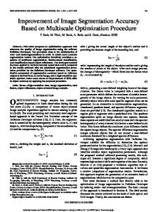
2.4 Accuracy Assessment For training objects, we digitized features like urban area and water bodies. For computing the accuracy of the segmentation in the terms of different parameters such as 1) the relative area of an overlapped region to a reference object (RAor), (2) the relative area of an overlapped region to a segmented object (RAos), (3) the quality rate (qr), (4) the SimSize, and (5) the Area Fit Index (AFI) (6) Position discrepancy of a segmented object to a reference object (Dsr) , different analysis has done on the both referenced and segmented layers. Satellite Imagery (RESOURSESAT II and LANDSAT8)
Pre-processing of Data
Segmentation
Accuracy Assessment
Result Figure 1:Flow Chart of Methodology
3. Results and Discussion Different algorithm gave different results for different satellite imagery. The result for the each segmentation algorithm has shown below. There are various algorithm such as region growing algorithm, watershed algorithm and object based image analysis used in the study. Segmentation result for the water body has been shown in figure 2 and figure 3 for the LISS III image and ETM+ image respectively. Among all algorithms executed in the study, region growing algorithm gave better result for both LISS III images and ETM+ images.
(a)(b) (c)(d) Figure 2: (a) Actual image (b) Result from the region growing algorithm (c) Result from the watershed algorithm (d) Result from the Object based image analysis.
42
Jain et al., OSGIS-2015, 40-47
(a) (b) (c) (d) Figure 3: (a) Actual image (b) Result from the region growing algorithm (c) Result from the watershed algorithm (d) Result from the Object based image analysis.
Segmentation result for the residential area has been shown in figure 4 and figure 5 for the LISS III image and ETM+ image respectively. Among all algorithms executed in the study, object based image analysis gave better result for both LISS III images and ETM+ images.
(a) (b) (c) (d) Figure 4: (a) Actual image (b) Result from the region growing algorithm (c) Result from the watershed algorithm (d) Result from the Object based image analysis.
(a) (b) (c) (d) Figure 5: (a) Actual image (b) Result from the region growing algorithm (c) Result from the watershed algorithm (d) Result from the Object based image analysis.
Comparison between different algorithm for the different feature and different satellite imagery has given below in the tabular form in table 1. The result has shown in terms of different parameters. The table included (1) the relative area of an overlapped region to a reference object (RAor), (2) the relative area of an overlapped region to a segmented object (RAos), (3) the quality rate (qr), (4) the SimSize, and (5) the Area Fit Index (AFI) (6) Position discrepancy of a segmented object to a reference object (Dsr).
43
Jain et al., OSGIS-2015, 40-47
Table 1: The Comparative analysis for different algorithm
Feature and Algorithms
Centroid for Referenced area (x,y)
Centroid for segmented area (x,y)
Ar (Referenced Area) in meter2 )
As (Segmented Area) ( in meter2 )
Region Growing
344310.108, 2035023.608
Watershed algorithm Object based image analysis
Au (Union Area) (in meter2 )
Ao ( Overlay area) (in meter2)
344,244.708 2,035,030.757
4416027.1
4148646.6 4659505.9
3905167.8
344310.108, 2035023.608
344,579.993 2,035,813.709
4416027.1
3429205.7 4549272.7
3295960.1
344310.108, 2035023.608
344220.758,20 35082.815
4416027.1
3674880.0 4564352.5
3526554.6
Region Growing
344310.108, 2035023.608
344,289.304 2,035,166.884
4416027.1
3890632.6 4766851.0
3837355.8
Watershed algorithm
344310.108, 2035023.608
344,640.400 2,035,012.021
4416027.1
5071025.0 5139173.1
4347879.0
Object based image analysis
344310.108, 2035023.608
344251.946, 2035063.546
4416027.1
3592288.8 4542451.7
3465864.3
Residential_ LISS3 Region Growing
344416.284, 2044829.877
344,397.801 2,044,639.567
899141.6
494905.8 1032493.2
409966.0
Watershed algorithm
344416.284, 2044829.877
344,431.842 2,044,410.534
899141.6
634855.4 1123857.3
410139.8
Object based image analysis
344416.284, 2044829.877
344550.290, 2044627.066
899141.6
1021248.0 1272875.5
647514.1
Residential_ ETM+ Region Growing
344416.284, 2044829.877
344,562.235 2,044,740.604
899141.6
705208.3
1057299.7
547050.2
Watershed algorithm
344416.284, 2044829.877
344,982.464 2,045,387.231
899141.6
1146736.9
1158817.5
887061.0
Object based image analysis
344416.284, 2044829.877
344455.722, 2044848.770
899141.6
651712.5
974846.8
576007.2
River_LISS3
River_ETM+
∑
∑ 44
Jain et al., OSGIS-2015, 40-47
∑
∑ (
)
∑√ Where n represents the number of segmented objects, Aris the area of the reference object, As(i) is the area of the ith segmented object, Ao(i) is the area of the ith overlapped region associated with the reference object, and Au(i) is the area of the union between the references object and the ith segmented object. When reference objects are well-segmented, both values of RAor and RAosare close to 100. The qr parameter (Weidner 2008) ranges between 0 and 1. The values close to zero indicate a perfect match while values close to one indicate an over or under segmentation. The Sim Size (Zhan et al. 2005) measures the similarity in terms of the size of the ith segmented object and ranges between 0 and 1, with one being ideal. AFI compares the area of the reference object with the largest area of the segmented objects. AFI is ideally zero, while AFI 0 denotes over-segmentation. Dsris the average of the Euclidian distance (m) in the xy plane between the centroid coordinates of the ith segmented object (Xs(i) and Ys(i)) and the centroid coordinates of the reference object (Xr and Yr). Dsrtends towards 0 when the centres of objects are in the same location, while under- and over-segmentation produced increase of Dsr (Montaghi et.al, 2013). Result has been shown in the table given below: Table 2: Segmentation resultsfor the RESOURCESAT LISS III satellite imagery
Residential Watershed algorithm Region Growing Object based image analysis River Watershed algorithm Region Growing Object based image analysis
RAor%
RAos%
qr
SimSize
AFI
Dsr(In Meters)
45.6
64.60
0.6351
0.71
0.294
419.6
45.59 72.01
82.84 63.4
0.603 0.4913
0.55 0.88
0.45 -0.136
191.20 243.08
74.6
96.114
0.2755
0.776
0.2235
834.92
88.43 79.86
94.13 95.96
0.1619 0.2274
0.94 0.83
0.9060 0.1678
65.789 107.186
45
Jain et al., OSGIS-2015, 40-47
Table 3: Segmentation results for the LANDSAT ETM+ satellite imagery
RAor%
RAos%
qr
SimSize
AFI
Dsr(In Meters)
Watershed algorithm Region Growing
98.66
77.35
0.234
0.784
-0.275
794.48
60.84
77.57
0.482
0.784
0.216
171.1
Object based image analysis River
64.06
88.38
0.409
0.725
0.275
43.73
Watershed algorithm Region Growing
98.46
85.74
0.154
0.878
-.148
330.49
86.89
98.63
0.195
0.881
0.118
144.78
Object based image analysis
78.48
96.48
0.237
0.813
0.186
70.55
Residential
4. Conclusion The accuracy of algorithms varies from feature to feature and image to image. A single algorithm cannot give the optimum result for each feature. There are various parameters which help in measuring the accuracy of segmentation algorithms such as (1) the relative area of an overlapped region to a reference object (RAor), (2) the relative area of an overlapped region to a segmented object (RAos), (3) the quality rate (qr), (4) the SimSize, and (5) the Area Fit Index (AFI) (6) Position discrepancy of a segmented object to a reference object (Dsr).Comparing the results of the both satellite imagery on the basis of the above mentioned parameters in open source interface, it is concluded that LANDSAT ETM+ image gave better performance than LISS III image.
5. Acknowledgements Special thanks to Indian Institute of Remote Sensing, ISRO and also wish to express appreciation and gratitute towards Dr. Poonam S. Tiwari (SE, IIRS) and Dr. Hina Pandey (SE, IIRS) for their continued support and their valuable comments and suggestions. I also want to thank Mr. Lohit Jain and Mr.Gaurav Jyoti Doley for helping mein improving the quality of the paper. I also want to show my gratitute towards bhuvan.nrsc.gov.in for providing us the data.
References Alessandro Montaghi, René Larsen and Mogens H. Greve.(2013). Accuracy assessment measures for image segmentation goodness of the Land Parcel Identification System (LPIS) in Denmark. Remote Sensing Letters, Vol. 4, No. 10, 946–955. Balázs Dezső, István Fekete, Dávid Gera, Roberto Giachetta and IstvánLászló (2012). Object-based image analysis in remote sensing applications using various segmentation technique. Annales University of Science Budapest, Sect. Comp. 37 103–120. Dusan Heric, Bozidar Potocnik, (2007). Objective assessment of image segmentation algorithms. Elektrotechniskivestnik 74 (1-2):13-18. Nicholas Clinton, Ashley Holt, Li Yanb, Peng Gongac. (2008). An accuracy assessment measure for object based image segmentation. The International Archives of the Photogrammetry, Remote Sensing and Spatial Information Sciences, Vol. XXXVII. Part B4. Beijing. 46
Jain et al., OSGIS-2015, 40-47
Rohan Kandwal, Ashok Kumar, Sanjay Bhargava. (2014). Review: Existing Image Segmentation Techniques”, International Journal of Advanced Research in Computer Science and Software Engineering”,Volume 4, Issue 4. Wang, z., Jensen, j.r. and im, j. (2010).An automatic region-based image segmentation algorithm for remote sensing applications”.Environmental Modelling & Software, 25, pp.1149–1165. Weidner, U. (2008). Contribution to the assessment of segmentation quality for remote sensing applications.Proceedings of the 21st Congress for the International Society for Photogrammetry and Remote Sensing, 3–11 July. Beijing, China, pp. 479–484. Zhan, q., Molenaar, m., Tempfli, k. and Shi, w. (2005). Quality assessment for geo-spatial objects derived from remotely sensed data. International Journal of Remote Sensing, 26, pp. 2953– 2974.
47