element methods, evaluation of integrals over arbitrary-shaped domain Ω .... Integration over the normalized (standard) triangle can be calculated as a sum of ...
IOSR Journal of Mechanical and Civil Engineering (IOSRJMCE) ISSN : 2278-1684 Volume 2, Issue 6 (Sep-Oct 2012), PP 38-51 www.iosrjournals.org
Accurate Evaluation Schemes for Triangular Domain Integrals Farzana Hussain1, M. S. Karim2 1,2
(Department of Mathematics, Shahjalal University of Science and Technology, Sylhet -3114, Bangladesh.)
ABSTRACT : This paper mainly presents higher order Gaussian quadrature formulae for numerical integration over the triangular surfaces. In order to show the exactness and efficiency of such derived quadrature formulae, it shows the effective use of available Gaussian quadrature for square domain integrals to evaluate the triangular 𝑛(𝑛 +1) domain integrals. Then it presents n × n points and − 1 points (for n >1) Gaussian quadrature formulae for 2 triangle utilizing n-point one-dimensional Gaussian quadrature. By use of simple but straight-forward algorithms, Gaussian points and corresponding weights are calculated and presented for clarity and reference. The proposed 𝑛(𝑛+1) − 1 point formula completely avoids the crowding of Gaussian points. Finally, it presents an error formula 2 which can evaluate the error in monomial/polynomial integration using m×n point method successfully. The error calculated by the new formula and the error in calculation of integrals by the proposed methods are found to be in good agreement. Thus, it overcomes all the drawbacks in view of accuracy and efficiency for the numerical evaluation of the triangular domain integrals of any arbitrary functions encountered in the realm of science and engineering. Keywords: Extended Gaussian quadrature, Triangular domain, Numerical accuracy, Convergence, Error formula.
I.
Introduction
The integration theory extends from real line to the plane and three dimensional spaces by the introduction of multiple integrals. Integration procedures on finite domains underlie physically acceptable averaging process in engineering. In probabilistic estimations and in spatially discreatized approximations, e.g., finite and boundaryelement methods, evaluation of integrals over arbitrary-shaped domain Ω become the pivotal task. In practice, most of the integrals (encountered frequently) either cannot be evaluated analytically or the evaluations are very lengthy and tedious. Thus, for simplicity numerical integration methods are preferred and the methods extensively employ the Gaussian quadrature technique that was originally designed for one dimensional cases and the procedure naturally extends to two and three-dimensional rectangular/cubic domains according to the notion of the Cartesian product. Gaussian quadratures are considered as the best method of integrating polynomials because they guarantee that they are exact for polynomials less than a specified degree. In order to obtain the result with the desired accuracy, Gaussian integration points and weights necessarily increase and there is no computational difficulty except time in evaluating any domain integral when the two and three-dimensional regions are bounded respectively, by systems of parallel lines and parallel planes. Analysts cannot ignore at all the randomness in material properties and uncertainty in geometry that are frequently encountered in complex engineering systems. Specifically, the vital components are rated during quality control inspections according to reliability indices calculated from the average probability density functions that model failure. This entails the evaluation of an integral of the function (say joint probability frequency function) over the volume Ω of the component. In general, the Ω-shape-class is very irregular in two and three-dimensional geometry. For non parallelogram quadrilateral, very frequent in finite-element modeling, there is no consistent procedure to select the sampling point to implement a Gaussian quadrature on the entire element. Special integration schemes, e.g., reduced integration over quadrilaterals have been successfully developed in [1] and are widely used in commercial programs. There is no methodical way to design such approximate integration schemes for polygons with more than four sides. An attempt to distribute the sampling points according to the governing perspective transformation fails to assure the error order germane to the quadrature formula. The reason can be traced to the crowding of quadrature points and this numerical computational difficulty persists in all non parallelogram polygonal finite elements [2]. A considerable amount of research has been performed to attain perfect results of domain integration for plane quadrilateral elements where numerical quadrature techniques are employed [3]. The accuracy of a selected quadrature strategy is indicated by compliance with the patch-test proposed in [4]. The overall error in a finite element calculation can be reduced by not relying so heavily on artificial tessellation, which requires the deployment of elements with large number of sides. An elegant systematic procedure to yield shape functions for convex polygons of arbitrary number of sides developed in [5] by which the energy density can be obtained in closed algebraic form in terms of rational polynomials. However, a direct Gaussian www.iosrjournals.org
38 | Page
Accurate Evaluation Schemes for Triangular Domain Integrals quadrature scheme to numerically evaluate the domain integral on n-sided polygons cannot be constructed to yield the exact results, even on convex quadrilaterals. In two-dimension, n-sided polygons can be suitably discretized with linear triangles rather than quadrilaterals (Fig. 1) and hence triangular elements are widely used in finite element analysis. Another advantage is to be mentioned that there is no difficulty with triangular elements as the exact shape functions are available and the quadrature formulas are also exact for the polynomial integrands [6]. Integration schemes based on weighted residuals are prone to instability since the accuracy goal cannot be controlled. In deterministic cases the underlying averaging process may be inconsistent, which was stated as a variational crime [7]. In stochastic differential equation literature [8-9], such averaging processes are termed dishonest [10]. Thus, the high accuracy integration method is demanded and it is meaningful when the shape functions are the very best. Therefore, there has been considerable interest in the area of numerical integration schemes over triangles [11-24]. It is explicitly shown in [21, 24] that the most accurate rules are not sufficient to evaluate the triangular domain integrals and for some element geometry these rules are not reliable also. To address all these short comings, to make a proper balance between accuracy and efficiency, to avoid the
nn 1 1 points higher order Gaussian 2 nn 1 quadrature formulae to evaluate the triangular domain integrals. It is thoroughly investigated that the 1 2 crowding of quadrature points this article proposed n × n points and
point formulae are totally free of crowding of Gauss points and also appropriate in view of accuracy and efficiency. Finally, it presents an error formula which can evaluate the error in monomial/polynomial integration using m × n point method successfully. The error calculated by the new formula and the error in calculation of integrals by the proposed methods are found to be in good agreement. Hence we believe that the formulae will find better place in numerical solution procedure of continuum mechanics problems.
II.
Problem Statement
In finite and boundary element methods for two-dimensional problems, a pivotal task is to evaluate the integral of a function f:
f d ;
I1
: element domain
2.1
Observe that I1 can be calculated as a sum of integrals evaluated over simplex divisions‟ ∆ i:
i ; i completely covers
2.2
i
∆i = triangle for two dimensional domain (see Fig. 1).
Now (2.1) can be written as
I1
fd i f di
2.3
i
To evaluate the integral I1 in (2.3), it is now required to evaluate the triangular domain integral:
I2
f ( x, y) dx dy ;
: triangle (arbitrary)
2.4
Integration over triangular domains is usually carried out in normalized co-ordinates. To perform the integration, first map one vertex (vertex 1) to the (-1,-1), the second vertex (vertex 2) to point (1,-1) and the third vertex (vertex 3) to point (-1, 1). This geometrical transformation to standard triangle is most easily accomplished by use of shape functions as:
www.iosrjournals.org
39 | Page
Accurate Evaluation Schemes for Triangular Domain Integrals 𝑥 𝑥1 𝑦 = 𝑦1 Where N1
𝑥2 𝑦2
𝑁1 𝑁2 𝑁3
𝑥3 𝑦3
1 s t , 2
2.5
N2
1 s 1, 2
N3
1 t 1, 2
2.6
The original and the transformed triangles are shown in Fig. 2. t
3 3(-1, 1)
y
s
2
1
1(-1, -1)
x
2(1, -1)
(b) Normalized triangle triangle in (s, t) space.
(a) Triangle in (x, y) space.
Fig. 2: Original and Transformed triangle.
Form (2.5) using (2.6), we obtain
1 1 1 x( s, t ) ( x2 x3 ) ( x2 x1 ) s ( x3 x1 ) t 2 2 2 1 1 1 y ( s, t ) ( y 2 y3 ) ( y 2 y1 ) s ( y3 y1 ) t 2 2 2
2.7
and hence
( x, y) 1 Area ( x2 x1 ) ( y3 y1 ) ( x3 x1 ) ( y 2 y1 ) ( s, t ) 4 4
2.8
Finally (2.4) reduces to
I2
Area 4
s
1
f ( x(s, t ), y(s, t )) dt ds
2.9
s 1 t 1
One can simply verify that
Area I2 4
1
t
f ( x(s, t ), y(s, t ))
dt ds
2.10
t 1 s 1
Here, we wish to mention that the evaluation of integrals I2 in (2.9) and (2.10) by the existing Gaussian quadrature (i.e. 7-point and 13-point) will yield the same results. Thus, any one of these two can be evaluated numerically. Influences of these integrals will be investigated later to present new quadrature formulae for triangles.
III.
Numerical Evaluation Procedures
In this section, we wish to describe different procedures to evaluate the integral I2 numerically and new Gaussian quadrature formulae for triangles. 3.1 Procedure-1 (use of Gaussian quadrature for triangle, GQT): Gaussian quadrature for triangle in [11-24] can be employed as 𝐴𝑟𝑒𝑎 𝐼2 = 4
𝑁𝐺𝑃 𝑁𝐺𝑃
𝑊𝑖 𝑊𝑗 𝑓 𝑥 𝑠𝑖 , 𝑡𝑗 , 𝑦 𝑠𝑖 , 𝑡𝑗
3.1
𝑖=1 𝑗 =1
where (si , tj) are the ij-th sampling points Wi ,Wj are corresponding weights and NGP denotes the number of gauss points in the formula. It is thoroughly investigated that in some cases available Gaussian quadrature for triangle cannot evaluate the integral I2 exactly [11, 21, 24]. 3.2 Procedure-2 (use of Gaussian quadrature for square domain integral, IOST): Integration over the normalized (standard) triangle can be calculated as a sum of integrals evaluated over www.iosrjournals.org
40 | Page
Accurate Evaluation Schemes for Triangular Domain Integrals three quadrilaterals (Fig – 3). Then I2 can be written as:
Area I2 4
Area 4 area 96
s
1
f ( x(s, t ), y(s, t )) dt ds
s 1 t 1 3
f ( x(s, t ), y(s, t )) dt ds
3.2
j 1 e j 1
1
f ( X 1 , Y1 )(4 ) f ( X 2 , Y2 )(4 ) f ( X 3 , Y3 )(4 )d d
1 1
(3.2) is obtained after transforming each quadrilaterals in to a square in ( δ, ε ) space where 1 1 𝑋1 = 𝑎11 + 𝑎12 𝜉 + 𝑎13 𝜂 + 𝑎14 𝜉𝜂 𝑌1 = 𝑏 + 𝑏12 𝜉 + 𝑏13 𝜂 + 𝑏14 𝜉𝜂 24 24 11 𝑋2 = 𝑋3 =
1 𝑎 + 𝑎22 𝜉 + 𝑎23 𝜂 + 𝑎24 𝜉𝜂 24 21
1 𝑎 + 𝑎32 𝜉 + 𝑎33 𝜂 + 𝑎34 𝜉𝜂 24 31
𝑌3 =
𝑌2 =
1 𝑏 + 𝑏22 𝜉 + 𝑏23 𝜂 + 𝑏24 𝜉𝜂 24 21
1 𝑏 + 𝑏32 𝜉 + 𝑏33 𝜂 + 𝑏34 𝜉𝜂 24 31
3.3
t 3(-1, 1)
s
e3
e1
e2 2(1, -1)
1(-1, -1)
Fig 3: Standared triangle splitted into three quadrilaterals.
and 𝑎11 = 5𝑥1 + 5𝑥2 + 14𝑥3
𝑏11 = 5𝑦1 + 5𝑦2 + 14𝑦3
𝑎12 = − 𝑥1 + 5𝑥2 − 4𝑥3
𝑏12 = −𝑦1 + 5𝑦2 − 4𝑦3
𝑎13 = −5𝑥1 + 𝑥2 + 4𝑥3
𝑏13 = −5𝑦1 + 𝑦2 + 4𝑦3
𝑎14 =
𝑥1 + 𝑥2 − 2𝑥3
𝑏14 =
𝑦1 + 𝑦2 − 2𝑦3
𝑎21 = 14𝑥1 + 5𝑥2 + 5𝑥3
𝑏21 = 14𝑦1 + 5𝑦2 + 5𝑦3
𝑎22 = −4𝑥1 + 5𝑥2 − 𝑥3
𝑏22 = −4𝑦1 + 5𝑦2 − 𝑦3
𝑎23 = −4 𝑥1 − 𝑥2 + 5𝑥3
𝑏23 = − 4𝑦1 − 𝑦2 + 5𝑦3
𝑎24 = 2𝑥1 − 𝑥2 − 𝑥3
𝑏24 = 2𝑦1 − 𝑦2 − 𝑦3
𝑎31 = 5𝑥1 + 14𝑥2 + 5𝑥3
𝑏31 = 5𝑦1 + 14𝑦2 + 5𝑦3
𝑎32 = −5𝑥1 + 4𝑥2 + 𝑥3
𝑏32 = −5𝑦1 + 4𝑦2 + 𝑦3
𝑎33 = − 𝑥1 − 4𝑥2 + 5𝑥3
𝑏33 = − 𝑦1 − 4𝑦2 + 5𝑦3
𝑎34 = 𝑥1 − 2𝑥2 + 𝑥3
𝑏34 = 𝑦1 − 2𝑦2 + 𝑦3
www.iosrjournals.org
41 | Page
Accurate Evaluation Schemes for Triangular Domain Integrals Now right hand side of (3.2) with (3.3) can be evaluated by use of available higher order Gaussian quadrature for square. For clarity, we mention that each quadrilaterals in Fig. 3 is transformed into 2- square in (ξ, ε) {(-1,-1), (1,-1), (1,1), (-1,1)} space through isoperimetric transformation and that resulted the equivalent integral I2 in (3.2). 3.3 Procedure-3: In this section, we wish to present two new techniques to evaluate the integrals over the triangular surface and to calculate Gaussian points and corresponding weights for triangle. Using mathematical transformation equations: 1 − 𝜉 (1 + 𝜂) −1 3.4 2 Then, the integral I2 of (2.9) is transformed into an integral over the surface of the standard square {(𝜉, 𝜂) −1 ≤ 𝜉, 𝜂 ≤ 1} and the (2.7) reduces to 𝑠 = 𝜉,
𝑡=
1 1 1 ( x2 x3 ) ( x2 x1 ) ( x3 x1 ) ( 1) 2 2 4 1 1 1 y ( y 2 y3 ) ( y 2 y1 ) ( y3 y1 ) ( 1) 2 2 4
x
3.5
Now the determinant of the Jacobean and the differential area are:
( s, t ) s t s t 1 (1 ) ( , ) 2 ( s, t ) 1 d d (1 )d d and ds dt dt ds ( , ) 2
3.6 3.7
Now using (3.4) and (3.7) into (2.9), we get 1 1
I 2 Area
1 1 1 1
Area
1 1
(1 )(1 ) (1 )(1 ) 1 f x , 1, y , 1 d d 2 2 8
(1 )(1 ) 1 f , 1 d d 2 8
3.8
In order to evaluate the integral I2 in (3.8) efficient Gaussian quadrature co-efficient (points and weights) are readily available so that any desired accuracy can be readily obtained [21, 24]. 3.3.1 New quadrature formula, GQSTS: In this section we are straightly computing Gaussian quadrature formula for standard triangles (GQSTS). The Gauss points are calculated simply for i = 1, m and j = 1, n. Thus the m × n point Gaussian quadrature formula for (3.8) gives 𝑚 𝑛 𝑚 ×𝑛 1 − 𝜉𝑖 1 + 𝜂𝑗 1 − 𝜉𝑖 𝐼2 = 𝐴𝑟𝑒𝑎 𝑊𝑖 𝑊𝑗 𝑓 𝜉𝑖 , − 1 = 𝐴𝑟𝑒𝑎 𝐺𝑟 𝑓(𝑢𝑟 , 𝑣𝑟 ) 3.9 8 2 𝑖=1 𝑗 =1
𝑟=1
where (ur , vr) are the new Gaussian points, Gr is the corresponding weights for triangles. Again, if we consider the integral I2 of (2.10) and substitute 1 + 𝜉 (1 − 𝜂) − 1, 𝑡=𝜂 2 Then one can obtain (on the same line of (3.9)) 𝑠=
1
1
𝐼2 = 𝐴𝑟𝑒𝑎 −1 −1 / 𝐺𝑟 and
𝑓
1+𝜉 1−𝜂 1−𝜂 − 1, 𝜂 𝑑𝜉𝑑𝜂 = 𝐴𝑟𝑒𝑎 2 8 /
𝑚×𝑛 /
/
/
𝐺𝑟 𝑓(𝑢𝑟 , 𝑣𝑟 )
3.10
𝑟=1
/
where ( 𝑢𝑟 , 𝑣𝑟 ) are respectively weights and Gaussian points for triangle. All the Gaussian points and corresponding weights can be calculated simply using the following algorithm:
www.iosrjournals.org
42 | Page
Accurate Evaluation Schemes for Triangular Domain Integrals step1. r 1 step 2. i 1, m step 3. j 1, n 1 ξi Gr Wi W j , 8 1 ηj Wi W j , G r/ 8 r r 1 step 4. compute step 3
u r ξi , u r/
vr
(1 ξ i )(1 η j ) 2
- 1,
(1 ξ i )(1 η j ) 2
1
v r/ η j
step 5. computestep 2
For clarity and reference, computed Gauss points and weights (for n = 3, 7) based on above algorithm listed in Table-1 and Fig. 4a shows the distribution of Gaussian points for n = 10. In figure- 4a, it is seen that there is a crowding of points at least at one point within the triangle and that is one of the major causes of error germen in the calculation. To avoid this crowding further modification is needed. This modification is obtained in the next section. 1
v
0.5 0
-0.5 -1 -1
-0.5
0 u
0.5
1
Fig 4a. Distribution of 10 X 10 Gauss Points.
3.3.2 New quadrature formula, GQSTM: It is clearly noticed in the (3.9) that for each i (i = 1, 2, … m) j varies from 1 to n and hence at the terminal value i = m there are n crowding points as shown in Table-1 and Fig.- 4a. To overcome this situation, we can use the advantage of (3.9) by making j dependent on i for the calculation of new gauss points and corresponding weights. To do so, we wish to calculate gauss points and weights for i = 1, m-1 and j = 1, m + 1 – i that is
mm 1 1 points Gaussian quadrature formulae from (3.9) as: 2 𝑚 −1 𝑚−𝑖+1
1 − 𝜉𝑖 1 + 𝜂𝑗 1 − 𝜉𝑖 𝑊𝑖 𝑊𝑗 𝑓 𝜉𝑖 , − 1 = 𝐴𝑟𝑒𝑎 8 2
𝐼2 = 𝐴𝑟𝑒𝑎 𝑖=1
𝑗 =1
𝑚 (𝑚 +1) −1 2
𝐿𝑟 𝑓 𝑝𝑟 , 𝑞𝑟
3.11
𝑟=1
where 𝑝𝑟 , 𝑞𝑟 are the new Gaussian points, Lr is the corresponding weights for triangles. Similarly, (3.10) can be written as 1
I 2 Area
1
1 1
(1 i )(1 j ) 1 f 1, j d d Area 2 8 /
/
m( m1) 1 2
L/r f ( pr/ , qr/ )
3.12
r 1
/
Where 𝑝𝑟 , 𝑞𝑟 are the new Gaussian points, 𝐿𝑟 are respectively weights of Gaussian points for triangle. All the Gaussian points and corresponding weights can be calculated simply using the following algorithm:
www.iosrjournals.org
43 | Page
Accurate Evaluation Schemes for Triangular Domain Integrals st ep1.
r 1
st ep 2.
i 1, m 1
st ep 3.
j 1, m 1 i
st ep 4.
1 i Lr WiW j , 8 j 1, m 1
pr i ,
qr
(1 i )(1 j ) 2
1
i 1, m 1 j
st ep 5.
1 j L/r 8 r r 1
WiW j ,
st ep 6.
comput e st ep 3 st ep 2
st ep 7.
comput est ep 5 st ep 4
Thus, the new
p r/
(1 i )(1 j ) 2
q r/ j
1,
mm 1 1 points Gaussian quadrature formulae is now obtained which is crowding free. 2
For clarity and reference, computed Gauss points and weights (for n = 5, 9) based on above algorithm listed in table2 and Fig. 4b shows the distribution of Gaussian points for n = 10 i.e. 54-points formula.
IV.
Application Examples
To show the accuracy and efficiency of the derived formulae, following examples with known results are considered: 1 1−𝑦
1 1−𝑦
𝐼1 =
𝑥+𝑦
1 2 𝑑𝑥
𝑑𝑦 = 0.4
𝐼2 =
𝑦=0 𝑥=0 𝑦 1
−
1 2 𝑑𝑥
𝑑𝑦 = 0.6666667
𝑦=0 𝑥=0 𝑦 1
𝑥2 + 𝑦 2
𝐼3 =
𝑥+𝑦
−
1 2 𝑑𝑥
𝑑𝑦 = 0.881373587
𝑒𝑥𝑝 𝑥+𝑦−1 𝑑𝑥 𝑑𝑦 = 0.71828183
𝐼4 =
𝑦=0 𝑥=0
𝑦=0 𝑥=0
Computed values (by use of three procedures) are summarized in Table-3. Some important remarks from the Table – 3 are: Usual Gauss quadrature (GQT) for triangles e.g. 7-point and 13-point rules cannot evaluate the integral of non-polynomial functions accurately. Splitting standard triangle into quadrilaterals (IOST) provides the way of using Gaussian quadrature for square and the convergence rate is slow but satisfactory in view of accuracy. New Gaussian quadrature formulae for triangle (GQSTS & GQSTM) are exact in view of accuracy and efficiency and GQSTM is faster in calculation of non-polynomial function. 1
q
0.5 0
-0.5 -1 -1
-0.5
0 p
0.5
1
Fig 4b. Distribution of 54 Gauss points (m = 10).
Again, we consider the following integrals of rational functions due to [24] to test the influences of formulae in (3.9), (3.10), (3.11) and (3.12) described in procedure-3. Consider 1 1 y
II
p ,q
y 0 x 0
x p yq dx dy x y 1 1 y
Example-1: II
r ,0
y 0 x 0 1 1 y
0, r Example-2: II
y 0 x 0
xr dx dy, 0 0.375 0.375x yr dx dy, 0 0.375 0.375y www.iosrjournals.org
44 | Page
Accurate Evaluation Schemes for Triangular Domain Integrals 1 1 y
0, 0 Example-3: II
1
12 21.53679831x 8.821067231y dx dy,
0, 0
y 0 x 0
1 1 y
Example-4: II
0, 0
1
12 9.941125498( x y) dx dy,
0
y 0 x 0
Results are summarized in Tables-(4, 5, 6). In Tables (4 - 6) for method GQSTS, Formula 1 is for (3.9) and Formula 2 is for (3.10) are written, for method GQSTM, Formula 1 is for (3.11) and Formula 2 is for (3.12) are written. These tables substantiated the influences of numerical evaluation of the integrals as described in section-3. Some important comments may be drawn from the Tables (4 - 6). For the integrand
xr with 0 the formulae in (3.9) and (3.11) described in procedure-3 is x y
more accurate and rate of convergence is higher. But the new formula in (3.11) requires very less computational effort. Similarly for the integrand
yr with 0 the second formula in (3.10) and (3.12) as described x y
in procedure-3 is more accurate and convergence is higher. Here also the new formula in (3.12) requires very less computational effort. Similar influences of these formulae in procedure-3 may be observed for different conditions on β, γ. General Gaussian quadrature e.g. 7-point and 13-point rules cannot evaluate the integral of rational functions accurately. It is evident that the new formulae e.g. (3.11) and (3.12) are very fast and accurate in view of accuracy and equally applicable for any geometry that is for different values of , and . We recommend this is appropriate quadrature scheme for triangular domain integrals encountered in science and engineering.
V. Consider the integral
1 1 𝑥=−1 𝑦=−1
𝑁 𝑖 𝑖=0 𝑥
Error Analysis: 𝑦 𝑁−𝑖 𝑑𝑦 𝑑𝑥
We are using m points along x direction and n points along y direction, the error in this method is found to be of the form
22𝑚 +2 𝑚! 4 22𝑛 +2 𝑛! 4 2𝑚 𝑓 𝑥 , 𝑦 + 𝑓 2𝑛 𝑥2 , 𝑦2 1 1 2𝑚 + 1 2𝑚 ! 3 𝑥 2𝑛 + 1 2𝑛 ! 3 𝑦
5.1
Where 𝑓𝑥2𝑚 𝑥1 , 𝑦1 is the (2m) th partial derivative of the function with respect to x, 𝑓𝑦2𝑛 𝑥2 , 𝑦2 is the (2n) th partial derivative of the function with respect to y and 𝑥1 , 𝑦1 and 𝑥2 , 𝑦2 are points somewhere in the domain [1, 1] ×[-1, 1]. The computed results for the errors are given in Table 7. We know, the n-point Gaussian Quadrature rule gives exact results for polynomials of degree at most 2n-1. Thus with n = 2, we have a rule with 4 nodes which is exact for any polynomial of degrees at most 3 in x and y separately, so the total degree of this monomial is at most 6. But this rule is not exact for all monomials of degree at most 6, which includes x6, x5 y, x4 y2, x3 y3, x2 y4, x y5, y6. Thus p × q -point rule cannot give exact result for all monomial of order 2(p + q)-2. Let N be the maximum value of p + q for each term in the polynomial. Then N-point rule can calculate all the polynomials of order up to 2p-1 or 2q-1 in x and y separately. Hence N×N- point rule can evaluate all the monomials of degree at most 2(p+q)-2 ie 2N-2. The method GQSTS is tested on the integral of all monomials xi yj where i , j are non-negative integers such that i j N . In Table-8, we present the absolute error over corresponding polynomial integral of order up to 30. Table 8 is in good agreement with the above statement. The results are compared with the results of [26] and it is observed that the new method GQSTS is always accurate for monomial/polynomial functions in view of both accuracy and efficiency and hence a proper balance is observed.
VI.
Conclusions:
In continuum mechanics and in spatially discreatized approximations, e.g., finite- and boundary-element methods, evaluation of integrals over arbitrary-shaped domain Ω is the important and pivotal task. Most of the integrals defy our analytical skills and we are resort to numerical integration schemes. Among all the numerical integration schemes Gaussian quadrature formulae are widely used for its simplicity and easy incorporation in computer. www.iosrjournals.org
45 | Page
Accurate Evaluation Schemes for Triangular Domain Integrals In general, the Ω –shape-class is very irregular in two and three-dimensional geometry. If the domain Ω is subdivided into quadrilaterals or into hexahedron respectively in two and three-dimensions, higher order Gaussian quadrature formulae are readily available. Furthermore, reduced integrations techniques compliance with the patchtest is also available [1, 4]. It is notable that there is no methodical way to design such approximate integration schemes for polygons with more than four sides. Generally simplexes e.g., triangle and tetrahedron are popular finite elements to discretized the arbitrary domain Ω. Though these are the widely used elements in FEM and BEM, Gaussian quadrature formulae for the triangular/tetrahedral domain integrals are not developed as compared to the square domain integrals. To achieve the desired accuracy of the integral it is necessary to increase the number of points and corresponding weights. Therefore, it is an important task to make a proper balance between accuracy and efficiency of the calculations. For the necessity of the exact evaluation of the integrals, this article shows first the integral over the triangular domain can be computed as the sum of three integrals over the square domain. In this case the readily available quadrature formulae for the square can be used for the desired accuracy. The results obtained are found accurate in view of accuracy and efficiency. Secondly, it presented new techniques to derive quadrature formulae utilizing the one dimensional Gaussian quadrature formulae and that overcomes all the difficulties pertinent to the higher order formulae. The first technique (GQSTS) derives two-types of m × m point quadrature formula utilizing the one dimensional m-point Gaussian quadrature formula. Finally, in the second technique (GQSTM) two-types of 𝑚 (𝑚 +1) − 1 points quadrature formulae are derived utilizing the m-point one dimensional Gaussian quadrature 2 𝑚 (𝑚+1)
formula. It is observed that the − 1 points scheme is appropriate for the triangular domain integrals as it 2 requires less computational effort for desired accuracy. Through practical application examples, it is demonstrated that the new appropriate Gaussian quadrature formula for triangles are accurate in view of accuracy and efficiency and hence a proper balance is observed. Finally, an error formula for numerical double integral using Gaussian quadrature is described. The error calculated by the new formula (5.1) and the error in calculation of integrals by the proposed methods are found to be in good agreement. Thus, we believe that the newly derived appropriate quadrature formulae for triangles and error formula will ensure the exact evaluation of the integrals in an efficient manner and enhance the further utilization of triangular elements for numerical solution of field problems in science and engineering.
References [1]. [2]. [3]. [4]. [5]. [6]. [7]. [8]. [9]. [10]. [11]. [12]. [13]. [14]. [15]. [16]. [17]. [18]. [19]. [20]. [21]. [22]. [23].
T.J.R. Hughes, The Finite Element Method, (Englewood Cliffs, N.J: Prentice-Hall, 1966). D.F. Rogers and J.A. Adams, Mathematical Elements of Computer Graphics, (McGraw-Hill, New York, 1990). K.J. Bathe, (1996), Finite Element Procedures, (Englewood Cliffs, N.J: Prentice-Hall, 1966). Irons, B.M. and Razzaque, A. (1972), Experience with the patch-test for convergence of finite element method, Academic press, New York. E.L. Wachspress, A rational finite element basis, (Academic press, San Diego, 1975). O.C. Zienkiewicz and R.L. Taylor, The finite element method, Vol. 1, 5th Ed., (Butterworth- Heinemann. Elsevier Science, Burlington, Mass, 2000). G. Strang and G.J. Fix, (1973), An analysis of the finite element method, (Englewood Cliffs, N.J: Prentice-Hall, 1973). J.B. Keller, Stochastic Equations and Wave propagation in Random Media, Proc., Symposium on Applied Mathematics, Vol. 16, American Mathematical Society, Providence, R.I, 1964. J.B. Keller and H.P. McKean,”SIAM-AMS Proceedings.” Stochastic differential equations, Vol.VI, American Mathematical Society, Providence, R.I., 1973. J.E. Molyneux, “Analysis of „dishonest‟ methods in the theory of wave propagation in a random medium”. J. Opt. Soc. Am., 58, 1968, 951-957. P. C. Hammer, O. J. Marlowe and A. H. Stroud, Numerical integration over simplex and cones, Math Tables Other Aids Computation, 10, 1956, 130 – 136. P. C. Hammer and A. H. Stroud, Numerical integration over simplexes, Math Tables Other Aids Computation, 10, 1956, 137 – 139. P. C. Hammer and A. H. Stroud, Numerical evaluation of multiple integrals, Math Tables Other Aids Computation, 12, 1958, 272 – 280. G. R. Cowper, Gaussian quadrature formulas for triangles, International journal on numerical methods and engineering, 7, 1973, 405 – 408. J. N. Lyness and D. Jespersen, Moderate degree symmetric quadrature rules for triangle, J. Inst. Math. Applications, 15, 1975, 19 – 32. F. G. Lannoy, Triangular finite element and numerical integration, Computers Struct, 7, 1977, 613. D. P. Laurie, Automatic numerical integration over a triangle, CSIR Spec. Rep. WISK 273, National Institute for Mathematical Science, Pretoria, 1977. M. E. Laursen and M. Gellert, Some criteria for numerically integrated matrices and quadrature formulas for triangles, International journal for numerical methods in engineering, 12, 1978, 67 – 76. F. G. Lether, Computation of double integrals over a triangle, Journal comp. applic. Math., 2, 1976, 219 – 224. P. Hillion, Numerical integration on a triangle, International journal on numerical methods and engineering, 11, 1977, 797 – 815. G. Lague and R. Baldur, Extended numerical integration method for triangular surfaces, International journal on numerical methods and engineering, 11, 1977, 388 – 392. C. T. Reddy, Improved three point integration schemes for triangular finite elements, International journal on numerical methods and engineering, 12, 1978, 1890 – 1896. C. T. Reddy and D. J. Shippy, Alternative integration formulae for triangular finite elements, International journal for numerical methods in engineering, 17, 1981, 133 – 139.
www.iosrjournals.org
46 | Page
Accurate Evaluation Schemes for Triangular Domain Integrals [24].
H. T. Rathod and M. S. Karim, An explicit integration scheme based on recursion for curved triangular finite elements, Computer structure, 80, 2002, 43 – 76. M. Abramowitz and I. A. Stegun, Handbook of mathematical functions, (Dover, 1974). S. Wandzura and H. Xiao, Symmetric quadrature rules on a triangle, Computers and mathematics with applications, 45, 2003, 1829 – 1840.
[25]. [26].
n
3
7
Table-1: Computed Gauss points (u, v) and weights G for n×n-point formula (GQSTS): u v G -0.7745966692414834E+00 -0.8000000000000000E+00 0.2738575106854138E+00 -0.7745966692414834E+00 -0.1127016653792583E+00 0.4381720170966623E+00 -0.7745966692414834E+00 0.5745966692414834E+00 0.2738575106854138E+00 0.0000000000000000E+00 -0.8872983346207417E+00 0.2469135802469134E+00 0.0000000000000000E+00 -0.5000000000000000E+00 0.3950617283950617E+00 0.0000000000000000E+00 -0.1127016653792583E+00 0.2469135802469134E+00 0.7745966692414834E+00 -0.9745966692414834E+00 0.3478446462322783E-01 0.7745966692414834E+00 -0.8872983346207417E+00 0.5565514339716456E-01 0.7745966692414834E+00 -0.8000000000000000E+00 0.3478446462322783E-01 -0.9491079123427585E+00 -0.9504029146358146E+00 0.1633971902233038E-01 -0.9491079123427585E+00 -0.7481081943789639E+00 0.3529604741916732E-01 -0.9491079123427585E+00 -0.4209640416964355E+00 0.4818316692765079E-01 -0.9491079123427585E+00 -0.2544604382862081E-01 0.5274230535088134E-01 -0.9491079123427585E+00 0.3700719540391937E+00 0.4818316692765079E-01 -0.9491079123427585E+00 0.6972161067217224E+00 0.3529604741916732E-01 -0.9491079123427585E+00 0.8995108269785730E+00 0.1633971902233038E-01 -0.7415311855993945E+00 -0.9556849211223279E+00 0.3153707751100920E-01 -0.7415311855993945E+00 -0.7749342496082218E+00 0.6812443847836622E-01 -0.7415311855993945E+00 -0.4826304010243249E+00 0.9299769892288504E-01 -0.7415311855993945E+00 -0.1292344072003028E+00 0.1017972322343420E+00 -0.7415311855993945E+00 0.2241615866237192E+00 0.9299769892288504E-01 -0.7415311855993945E+00 0.5164654352076163E+00 0.6812443847836622E-01 -0.7415311855993945E+00 0.6972161067217224E+00 0.3153707751100920E-01 -0.4058451513773972E+00 -0.9642268026617967E+00 0.3475337161903307E-01 -0.4058451513773972E+00 -0.8183164352463221E+00 0.7507207749196586E-01 -0.4058451513773972E+00 -0.5823551434482712E+00 0.1024820257759689E+00 -0.4058451513773972E+00 -0.2970774243113015E+00 0.1121789753788726E+00 -0.4058451513773972E+00 -0.1179970517433171E-01 0.1024820257759689E+00 -0.4058451513773972E+00 0.2241615866237192E+00 0.7507207749196586E-01 -0.4058451513773972E+00 0.3700719540391937E+00 0.3475337161903307E-01 0.0000000000000000E+00 -0.9745539561713792E+00 0.2705971537896379E-01 0.0000000000000000E+00 -0.8707655927996972E+00 0.5845271854796313E-01 0.0000000000000000E+00 -0.7029225756886985E+00 0.7979468810555958E-01 0.0000000000000000E+00 -0.5000000000000000E+00 0.8734493960849647E-01 0.0000000000000000E+00 -0.2970774243113015E+00 0.7979468810555958E-01 0.0000000000000000E+00 -0.1292344072003028E+00 0.5845271854796313E-01 0.0000000000000000E+00 -0.2544604382862081E-01 0.2705971537896379E-01 0.4058451513773972E+00 -0.9848811096809618E+00 0.1468787955288007E-01 0.4058451513773972E+00 -0.9232147503530723E+00 0.3172784626693875E-01 0.4058451513773972E+00 -0.8234900079291260E+00 0.4331216169277282E-01 0.4058451513773972E+00 -0.7029225756886985E+00 0.4741040083224655E-01 0.4058451513773972E+00 -0.5823551434482712E+00 0.4331216169277282E-01 0.4058451513773972E+00 -0.4826304010243249E+00 0.3172784626693875E-01 0.4058451513773972E+00 -0.4209640416964355E+00 0.1468787955288007E-01 0.7415311855993945E+00 -0.9934229912204305E+00 0.4680565643230238E-02 0.7415311855993945E+00 -0.9665969359911727E+00 0.1011066754980332E-01 0.7415311855993945E+00 -0.9232147503530723E+00 0.1380222483601957E-01 0.7415311855993945E+00 -0.8707655927996972E+00 0.1510820486158432E-01 0.7415311855993945E+00 -0.8183164352463221E+00 0.1380222483601957E-01 0.7415311855993945E+00 -0.7749342496082218E+00 0.1011066754980332E-01 0.7415311855993945E+00 -0.7481081943789639E+00 0.4680565643230238E-02 0.9491079123427585E+00 -0.9987049977069439E+00 0.4266374414229460E-03 0.9491079123427585E+00 -0.9934229912204305E+00 0.9215957350721234E-03 www.iosrjournals.org
47 | Page
Accurate Evaluation Schemes for Triangular Domain Integrals 0.9491079123427585E+00 0.9491079123427585E+00 0.9491079123427585E+00 0.9491079123427585E+00 0.9491079123427585E+00
-0.9848811096809618E+00 -0.9745539561713792E+00 -0.9642268026617967E+00 -0.9556849211223279E+00 -0.9504029146358146E+00
0.1258084244262349E-02 0.1377125407046231E-02 0.1258084244262349E-02 0.9215957350721234E-03 0.4266374414229460E-03
mm 1 1 point formula (GQSTM): 2 q L -0.9126939522585497E+00 0.7669385858827389E-01 -0.5705142370613163E+00 0.1549333650457879E+00 -0.6943184420297377E-01 0.1841508361811174E+00 0.4316505486553688E+00 0.1549333650457879E+00 0.7738302638526020E+00 0.7669385858827389E-01 -0.9069626449468782E+00 0.1519885905918008E+00 -0.5577935549985240E+00 0.2849424819989606E+00 -0.1022254014166197E+00 0.2849424819989606E+00 0.2469436885317342E+00 0.1519885905918008E+00 -0.9256147644301332E+00 0.1195633790398805E+00 -0.6699905217924281E+00 0.1913014064638090E+00 -0.4143662791547230E+00 0.1195633790398805E+00 -0.9706546497379454E+00 0.2415220341283323E-01 -0.8904816618561072E+00 0.2415220341283323E-01 -0.9687924202367442E+00 0.8063933990653976E-02 -0.8392867214556355E+00 0.1792366417936781E-01 -0.6210479706453962E+00 0.2585743793853289E-01 -0.3376704201677756E+00 0.3099065107963482E-01 -0.1985507175123180E-01 0.3276589850173939E-01 0.2979602766653120E+00 0.3099065107963482E-01 0.5813378271429326E+00 0.2585743793853289E-01 0.7995765779531718E+00 0.1792366417936781E-01 0.9290822767342806E+00 0.8063933990653976E-02 -0.9643270581779194E+00 0.2022265498028209E-01 -0.8173387381173184E+00 0.4442556514902738E-01 -0.5737699931387190E+00 0.6266989030061808E-01 -0.2664521977773301E+00 0.7245416447754392E-01 0.6311867519095693E-01 0.7245416447754392E-01 0.3704364705523460E+00 0.6266989030061808E-01 0.6140052155309454E+00 0.4442556514902738E-01 0.7609935355915465E+00 0.2022265498028209E-01 -0.9611812354352877E+00 0.3098378782547042E-01 -0.8028487233396140E+00 0.6692925642225962E-01 -0.5467987609586445E+00 0.9136613786352844E-01 -0.2372337950418355E+00 0.1000112912703450E+00 0.7233117087497343E-01 0.9136613786352844E-01 0.3283811332559430E+00 0.6692925642225962E-01 0.4867136453516165E+00 0.3098378782547042E-01 -0.9600410418417249E+00 0.3676731142740568E-01 -0.7995317256959110E+00 0.7742169799018377E-01 -0.5494777843396608E+00 0.1004172673430814E+00 -0.2670875731646896E+00 0.1004172673430814E+00 -0.1703363180843920E-01 0.7742169799018377E-01 0.1434756843373746E+00 0.3676731142740568E-01 -0.9616948561788959E+00 0.3508354238981680E-01 -0.8115650136036089E+00 0.7087414012328669E-01 -0.5917173212478248E+00 0.8423964820917546E-01 -0.3718696288920410E+00 0.7087414012328669E-01 -0.2217397863167538E+00 0.3508354238981680E-01 -0.9670568402059502E+00 0.2588799002096551E-01 -0.8434211981700837E+00 0.4853382811049090E-01
Table-2: Computed Gauss points (p, q) and weights L for points
(m =5) 14 point
(m = 9) 44 point
p -0.8611363115940526E+00 -0.8611363115940526E+00 -0.8611363115940526E+00 -0.8611363115940526E+00 -0.8611363115940526E+00 -0.3399810435848563E+00 -0.3399810435848563E+00 -0.3399810435848563E+00 -0.3399810435848563E+00 0.3399810435848563E+00 0.3399810435848563E+00 0.3399810435848563E+00 0.8611363115940526E+00 0.8611363115940526E+00 -0.9602898564975363E+00 -0.9602898564975363E+00 -0.9602898564975363E+00 -0.9602898564975363E+00 -0.9602898564975363E+00 -0.9602898564975363E+00 -0.9602898564975363E+00 -0.9602898564975363E+00 -0.9602898564975363E+00 -0.7966664774136268E+00 -0.7966664774136268E+00 -0.7966664774136268E+00 -0.7966664774136268E+00 -0.7966664774136268E+00 -0.7966664774136268E+00 -0.7966664774136268E+00 -0.7966664774136268E+00 -0.5255324099163290E+00 -0.5255324099163290E+00 -0.5255324099163290E+00 -0.5255324099163290E+00 -0.5255324099163290E+00 -0.5255324099163290E+00 -0.5255324099163290E+00 -0.1834346424956498E+00 -0.1834346424956498E+00 -0.1834346424956498E+00 -0.1834346424956498E+00 -0.1834346424956498E+00 -0.1834346424956498E+00 0.1834346424956498E+00 0.1834346424956498E+00 0.1834346424956498E+00 0.1834346424956498E+00 0.1834346424956498E+00 0.5255324099163290E+00 0.5255324099163290E+00
www.iosrjournals.org
48 | Page
Accurate Evaluation Schemes for Triangular Domain Integrals 0.5255324099163290E+00 0.5255324099163290E+00 0.7966664774136268E+00 0.7966664774136268E+00 0.7966664774136268E+00 0.9602898564975363E+00 0.9602898564975363E+00
-0.6821112117462453E+00 -0.5584755697103789E+00 -0.9770839733770847E+00 -0.8983332387068135E+00 -0.8195825040365421E+00 -0.9916082592691212E+00 -0.9686815972284151E+00
0.4853382811049090E-01 0.2588799002096551E-01 0.1256042196994617E-01 0.2009667515191388E-01 0.1256042196994617E-01 0.2009899851317608E-02 0.2009899851317608E-02
Table-3: Calculated values of the integrals 𝐼1 , 𝐼2 𝐼2 and 𝐼4 Gauss Point 7×7 GQT 13×13 7×7 IOST 10×10 7×7 GQSTS 10×10 54 GQSTM 90 Exact value
IOST GQT Method
GQSTM
GQSTS
IOST
GQT Method
Method
TP
7×7 13×13 5×5 6×6 7×7 8×8 9×9 10×10 5×5 6×6 7×7 8×8 9×8 10×10 14 44 77 90
Table 4: Computed results of Example -1 Value of I I r, 0 r=2 r=4 0.7288889289 0.7883351445 0.8536515995 0.8636423911 0.8699174628 0.8741142348 0.8770583374 0.8792029273 Formula 1 Formula 2 0.8888889003 0.8189709 0.8888888979 0.8386859 0.8888889008 0.8511113 0.8888888889 0.8594404 0.8888888960 0.8652928 0.8888888916 0.8695606 0.8888888885 0.7979759 0.8888888823 0.8620172 0.8888888823 0.8738937 0.8888888888 0.8761310 0.8888888
0.3733333349 0.4327795803 0.4980960513 0.5080868305 0.5143619067 0.5185586841 0.5215027742 0.5236473748 Formula 1 Formula 2 0.5333333421 0.4634153 0.5333333394 0.4831303 0.5333333320 0.4955557 0.5333333473 0.5038848 0.5333333366 0.5097372 0.5333333260 0.5140051 0.5333333288 0.4424203 0.5333333369 0.5064616 0.5333333366 0.5183381 0.5333333301 0.5205754 0.5333333
I4 0.6938790083 0.7238717079 0.7178753433 0.7180745324 0.7184323939 0.7182531970 0.7175459725 0.7180958214 0.71828183
r=6 0.2209523767 0.2803986370 0.3457150911 0.3557058624 0.3619809556 0.3661777177 0.3691218199 0.3712664246 Formula 1 Formula 2 0.3809523939 0.3110344 0.3809523751 0.3307493 0.3809523895 0.3431748 0.3809523887 0.3515039 0.3809523945 0.3573563 0.3809523860 0.3616241 0.3809523780 0.2900394 0.3809523803 0.3540807 0.3809523815 0.3659572 0.380952300 0.3699649 0.3809523
Table 5: Computed results of Example - 2. Value of I I 0, r
TP
7×7 13×13 5×5 6×6 7×7
Test example I2 I3 0.6606860757 0.8315681219 0.6637058258 0.8501738309 0.6664256210 0.8755247309 0.6665789279 0.8783900003 0.6659893974 0.8696444431 0.6664193645 0.8753981854 0.6663718426 0.8742865042 0.6665339400 0.8772635782 0.6666667 0.881373587
I1 0.4001498818 0.4000451564 0.4000006725 0.4000001234 0.4000037499 0.4000006929 0.4000009417 0.4000002469 0.4
r=2
r=4
r=6
0.7288889289 0.7883350849 0.8536515995 0.8636423911 0.8699174628
0.3733333349 0.4327795803 0.4980960513 0.5080868305 0.5143619067
0.2209523767 0.2803986370 0.3457150911 0.3557058624 0.3619809556
www.iosrjournals.org
49 | Page
Accurate Evaluation Schemes for Triangular Domain Integrals 8×8 9×9 10×10
GQSTS
GQST SEC 1
GQSTM
GQST SEC 2
5×5 6×6 7×7 8×8 9×9 10×10 14 44 77 90 Exact Value
0.8741142348 0.8770583374 0.8792029273 Formula 1 Formula 2 0.8189709 0.8888889003 0.8386859 0.8888888979 0.8511113 0.8888889008 0.8594405 0.8888888889 0.8652927 0.8888888960 0.8695606 0.8888888916 0.7979759 0.8888888885 0.8620172 0.8888888823 0.8738937 0.8888888823 0.8779014 0.8888888888 0.8888888
0.5185586841 0.5215027742 0.5236473748 Formula 1 Formula 2 0.4634153 0.5333333421 0.4831303 0.5333333394 0.4955558 0.5333333320 0.5038849 0.5333333473 0.5097372 0.5333333366 0.5140051 0.5333333260 0.4424203 0.5333333288 0.5064616 0.5333333369 0.5183381 0.5333333366 0.5223459 0.5333333301 0.5333333
0.3661777177 0.3691218199 0.3712664246 Formula 1 Formula 2 0.3110344 0.3809523939 0.3307493 0.3809523751 0.3431748 0.3809523895 0.3515039 0.3809523887 0.3573562 0.3809523945 0.3616241 0.3809523860 0.2900394 0.3809523780 0.3540807 0.3809523803 0.3659572 0.3809523815 0.3699649 0.3809523797 0.3809523
Table 6: Computed results of Example -3, 4 Method
TP
Example -3
Example -4
GQT
77 1313 55 66 77 88 99 1010
0.03669412062 0.03688941523 0.03694724351 0.03694789990 0.03694799397 0.03694800816 0.03694800990 0.03694801028 Formula 1 Formula 1 0.0369262 0.0369568 0.0369429 0.0369500 0.0369467 0.0369485 0.0369477 0.0369481 0.0369479 0.0369480 0.0369479 0.0369480 0.0368514 0.0369856 0.0369477 0.0369481 0.0369480 0.0369480 0.0369480 0.0369480 0.03694801040
0.02731705643 0.02731722965 0.02731723353 0.02731723339 0.02731723359 0.02731723343 0.02731723344 0.02731723331 Formula 2 Formula 2 0.0273172 0.0273172 0.0273172 0.0273172 0.0273172 0.0273172 0.0273172 0.0273172 0.0273172 0.0273172 0.0273172 0.0273172 0.0273172 0.0273172 0.0273172 0.0273172 0.0273172 0.0273172 0.0273172 0.0273172 0.02731723349
IOST
55 66 GQSTS 77 88 99 1010 14 GQSTM 44 77 90 Exact value
i j N
x1 y1 1
Table 7: Error calculated in
1
x i y j dydx using the new error formula.
Points
N
Error calculated using Eq (5.1)
2×2 3×3 4×4 5×5
4 6 8 10
0.71111111 0.18285711 0.04643999 0.01172724
www.iosrjournals.org
Error using the proposed method 0.71111111 0.18285714 0.04643993 0.01172679
50 | Page
Accurate Evaluation Schemes for Triangular Domain Integrals able 8: Absolute error in
1 x
i j N
x0 y0 1
x i y j dydx; N 30 for formula 1 and 2.
n
N
Formula 1
Formula 2
2
1 2 3 4 5 6 9 10 17 18 29 30
0.27755575615628913511E-15 0.13877787807814456755E-15 0.83266726846886740532E-15 0.61062266354383609723E-15 0.87617413324636572725E-13 0.56996074526693973894E-13 0.80144224590128487762E-15 0.70429773124658368033E-15 0.76934986159571394637E-14 0.65156213757688874466E-14 0.12595827159067596313E-13 0.11583616010835129373E-13
0.27755575615628913511E-15 0.13877787807814456755E-15 0.80491169285323849181E-15 0.61062266354383609723E-15 0.87610474430732665496E-13 0.56996074526693973894E-13 0.80144224590128487762E-15 0.70429773124658368033E-15 0.76934986159571394637E-14 0.65164887375068758502E-14 0.12595827159067596313E-13 0.11583616010835129373E-13
3 4 6 10 16
www.iosrjournals.org
51 | Page