other and the other remains silent (cooperates), the betrayer goes free and the silent accomplice receives ... (white) or selfish players (black). In gray colour, the ...
Complex Systems: Activity-Based Modeling and Simulation. Cargese Interdisciplinary Seminar, Corsica, A. Muzy, D. Hill and B.P. Zeigler editors, April 20-24, 2009.
Activatability for simulation tractability of NP problems: Application to Ecology Patrick Coquillarda, Alexandre Muzyb, Eric Wajnberga a: Ecologie moléculaire et comportementale, UMR CNRS-INRA-Université de Nice, 400 route de Chappes, P.O. box 167, 06903, Sophia-Antipolis, France. b: UMR CNRS LISA Università di Corsica - Pasquale Paoli UFR Drittu, Scenzi suciali, ecunòmichi è di gestioni 22, av. Jean Nicoli, BP 52 20250 Corti, France.
Summary Dynamics of biological-ecological systems is strongly depending on spatial dimensions. Most of powerful simulators in ecology take into account for system spatiality thus embedding stochastic processes. Due to the difficulty of researching particular trajectories, biologists and computer scientists aim at predicting the most probable trajectories of systems under study. Doing that, they considerably reduce computation times. However, because of the largeness of space, the execution time remains usually polynomial in time. In order to reduce execution times we propose an activatability-based search cycle through the process space. This cycle eliminates the redundant processes on a statistical basis (Generalized Linear Model), and converges to the minimal number of processes required to match simulation objectives.
Activatability for Simulation Tractability of NP Problems in Ecology
2
Introduction Most of –if not all–biological and ecological systems are strongly influenced by spatial dimensions. Indeed, it is well established that, whatever the particular space scale the systems are considered, the analysis of interactions between organisms, or between organisms and physico-chemical components, is crucial to understand system behaviour and structure. Furthermore, such interactions may occur both in various ways (e.g., secretion of chemical compounds, contacts between individuals, competition for resource, gain or loss of matter and energy, etc.) and at various distances (i.e., from immediate neighbouring to long distances). Finally, such interactions may occur in continuous or discrete modes in both space and time. Powerful simulators in ecology actually take into account the spatial dimension of interactions (Wu J. and David J. L., 2002; Ratzé et al., 2007). Several techniques are used, some of them allowing to involve both space and time, at a low level of details (e.g., Kendall process, stepping stone models, compartment models, etc.). Among these modelling techniques, the most powerful simulators in ecology belong to the class of “individual based models” (IBM hereafter; also denoted individually oriented models (IOM), Fishwick et al. 1998) which allow integrating spatial interactions at a high level of details. The IBM approach completes the set of usual formal mathematical methods (Grimm 1994, Sultangazin 2004). For instance, differential equations or partial differential equations are very efficient to give a coarse estimation of the evolution of large areas. However, (partial) differential equations are limited for simulating actual biological processes (Grimm and Uchmanski, 1994), particularly when the questions to be address require many details. Ecological modelling often has to account simultaneously for: (1) the diversity of individuals, (2) the spatial heterogeneity of the environment, (3) the changing interaction network (and changes of biotic structures), (4) the discrete and distant interactions between individuals, (5) the random processes and behaviours (i.e., random spatial interactions or movements), etc. IBMs are often implemented by object-oriented models (Coquillard and Hill, 1997) or by multi-agent models when there is a need to represent an autonomous social behaviour of individuals heading a common goal (Ferber, 1999). In this case, IBMs are usually called agents. In addition, such modelling approach has the main following advantages (Hill & Coquillard, 2007): (1) it allows theoretically the simulation of ecosystems with large sets of species harbouring different behaviours. Moreover, object classes can account for a part of mathematical modelling in order to obtain combined simulations if needed (mixing the discrete and continuous approach). (2) However, a lot of fieldwork always remains necessary as well as a deep knowledge of the modelled species. (3) It takes into account the spatial features of ecosystems that is difficult with partial differential equations (e.g., compartment models), or with the classical Markovian analysis. (4) It provides the possibility to manage, for each individual, the set of parameters the biologist decides to integrate in the model. The management of individuals, and correlatively of their physiological variations, enables model refinement to approach reality according to the detailed level wished by the user. In a first part, we will show, through a simple example, that (1) introducing spatial relationships between individuals is a prerequisite to maintain a sufficient level of diversity and (2) that such operation requires a probabilistic approach. In a second part
Activatability for Simulation Tractability of NP Problems in Ecology
3
we will propose a statistically driven method for reducing the state of space for a model. I. Reducing activity Example of spatialization necessity Let us have a look to the prisoner’s dilemma which is the most emblematic problem in the game theory. The problem was initially formalized by W. Tucker. In its classical form, the dilemma is expressed as follows: Two suspects are arrested by the police. The police having separated both prisoners visit each of them to offer the same deal. If one testifies for the prosecution against the other and the other remains silent (cooperates), the betrayer goes free and the silent accomplice receives a full 10-years sentence. If both remain silent, both prisoners are sentenced to only six months in jail. If each betrays the other, each receives a five-year sentence. Each prisoner must choose to betray the other or to remain silent. Each one is assured that the other would not know about the betrayal before the end of the investigation. How optimally should the prisoners act? In this game, the only concern of each prisoner is to maximize his payoff. Consequently, all rational players should play “testify” (fig. 1) and cooperating is strictly dominated by defecting. As a consequence of such strategy, the game leads to the disappearance of cooperators. But many examples of coexistence of cooperation and selfish behaviours can be found in animal societies and economical situations. How is it possible? M. Nowak and R. May demonstrated in 1992-1995 that introducing spatial dimension in the dilemma, even in an elementary - and somewhat opened to criticism - form, makes such situation possible. They first reformulated the dilemma by introducing a sentence variable b (b>1). Then, they distributed players on a grid in which each player has a probability to become a cooperator. This probability is function of states and gains of its immediate neighbours (see fig. 2 for details). As a result of such a transformation, they obtained for some couples (m, b) the coexistence of both strategies (see fig. 3). By doing that, however, they brought into the model some probabilistic compounds. Actually, this example illustrates clearly the usual way simulators reproduce spatial interactions. If the other prisoner testifies: If I remain silent, I will receive the full 10-years sentence; But if I testify, I will only receive a 5-years sentence If he does not: If I remain silent, I will receive a 6-monthes sentence; But if I testify, I will be free. «Whatever his choice, I have interest to testify»
Silent Testify
Silent (-0.5, -0.5) (0, -10)
Testify (-10,0) (-5, -5)
Silent Testify
Silent (1 , 1) (0 , b)
Testify (b , 0) (0 , 0)
Activatability for Simulation Tractability of NP Problems in Ecology
4
Figure 1. The original prisoner’s dilemma (upper table) is reformulated by introducing b>1 as a sentence variable (lower table).
P( j )
A
iN j
m i i
s
A
iN j
m i
=
probability that j switches to a cooperator state
si = 0 (selfish ■) With si = 1 (cooperator ■)
j
Nj = Set of neighbours of j Ai = Gains of cell i at time t m = 1, original stochastic game m , the more the cell j will get a chance to adopt the more profitable strategy of its neighbours (deterministic game) m = 0, the gains are worthless, neutral derivate between both strategies Figure 2. The spatialized dilemma (after M. Nowak and R. May). P(j) is the probability the prisoner j has to become a cooperator.
Figure 3. The spatialized prisoner’s dilemma in the (m,b) plane. Each cell of the grid represents a game of 100 × 100 players. Large areas present the coexistence of cooperators (white) or selfish players (black). In gray colour, the players which have just changed of state. After M. Nowak and R. May (modified).
Obviously, integration of space into simulators leads to a better representation of reality. However, the level of details increases the number of parameters, computations and interactions between parameters. This results in an explosion of the state space and to the intractability of simulations. Therefore, solutions have to be found to reduce the state space and thus enhance tractability.
Activatability for Simulation Tractability of NP Problems in Ecology
5
Space and NP problems According to the previous example, we can conclude that embedding spatial interactions into simulators (designed to model ecological systems) requires, in most cases, a stochastic approach. In most cases, several processes are acting simultaneously in the course of runs to simulate spatial interactions (e.g., various types of competition, seed dispersal, migration, gene flows, chromosome shuffling, chromosomal crossovers, etc.) Considering that each of these processes act on several levels (that can be large), the number of possible trajectories of the system is an exponential function of the number n of processes varying on p levels, and the time required to find a particular trajectory of the system is O(np). In other words, this problem belongs to the NP complexity class problem (see fig. 4). This is the reason why ecologists have early decided to reformulate the statement: “finding a particular trajectory” into “finding the most probable trajectory”. Let us define activity of a system as its number of transitions and activatability as the probability of transition activation. If we consider p processes varying on [1,...,n] levels and that each level can be activated with a probability following a law π, the activatability of the process i is (fig. 4): ∆i[πi(s i1 ,…, sin)], The activity can be estimated as proportional to the number of replicates (R), the confidence interval (%) and the number of processes (p): A ( R,%, p) 1
The number of replicates R depends on σ (the standard error of the response). Reformulating the original question in “finding the most probable trajectory”, we considerably reduced the computation time and escape from the NP-problem trap along with its heuristic solutions (the problem is now solvable in a polynomial time O(klog(p)) with p processes). However, the problem of activating many stochastic processes is still relevant and some algorithms can be time consuming (for instance, the algorithm AKS which tests the primarity of a number is O(log(n)10.5)). These considerations lead to the following question: “How to reduce the number of processes?” Kleijnen and Groenendaal (1992) proposed that building of 2(n-1) experimental designs in which each process is either active or inactive, give the same information than a 2n protocol (i.e., involving a half of process combinations). Thus, it is possible to test the effects of each process on the results eliminating redundant ones. The use of 2(n-k) protocols is also possible but results in introducing confusion between some interactions and a confusion of the main effects with their interactions.
1
The confidence interval of a mean is calculated as:
x T / 2; d
student law with α 0.05 and d is the degree of freedom (df).
s s x T / 2; d R R
, where
T / 2 is given by the
Activatability for Simulation Tractability of NP Problems in Ecology
A Final state (V1,…,Vn)
# of possible trajectories nP
P4
84 8P
P3
83
The time needed to compute all possible trajectories is O(np)
Exploring all states of a base model is intractable : Heuristics need to be experimented Definitions:
P2
8²
Activity:
Number of transitions
Activatability: Probability of transition activation
P1
81 Initial state (V10,…,Vn0)
B
Final states
We assume a computational sequential machine: < ∆ ,S>, With : ∆ = x∆i, S = xSi
S P1 … SPN
∆P
∆ 1(s 11 ,…, s1N) … ∆P(s P1 ,…, sPN)
…
Activatability: π(.)
∆2
S 21 … S2N ∆ 1[π1(s 11 ,…, s1N)] …
∆1
S 11 … S1N
∆P[πN(s P1 ,…, sPN)]
Figure 4. Activity, activatability and processes. Initial states
Figure 4. Activity, activatability and processes.
6
Activatability for Simulation Tractability of NP Problems in Ecology
7
Proposal of an activatability cycle ACTIVATABILITY CYCLE SEARCH SPACE Select activatable potentially pertinent processes
Activate selected processes Using ∆i [πN(s i1 ,…, siN)] Run simulator
Test the effects (using GLM) and reject inefficient processes yi ~ ∆i +..+ ∆j + …+∆i ∆j +… +…+
Run simulator
Figure 5.The activatability cycle. Every loop, processes with no significant effects are eliminated.
In this section we will propose a method to build the most parsimonious model from a list of processes. Based on statistical evidences, the method is automatable and allows to embed into the simulator all the process which have a significant effect on the results of simulation, even those on which we have no a priori ideas about their pertinence in the model. However, the method cannot be seen as a validation process. In addition, the proposal must not be confused with the works of Hoffman (2005), who proposed an extended genetic algorithm based method “to accomplish simultaneously parameter fitting and parsimonious model selection” among a list of candidate models. The proposed cycle of activatability (fig. 5) is based on a complete design protocol (2n protocol). At every cycle, main effects and their interactions on the response y, can be tested through a Generalized Linear Model (Nelder and Wedderburn, 1972). E(yi) = 0 +1∆1 +…+i∆i + …+k∆i.∆j +…+
(1)
where yi is the dependant variable2, ∆i (i [1..n] ) the principal effects (or independent variables), ∆i.∆j the interaction between the effects (sometimes called “product terms”) and is a random error. Equation (1) is thus a linear regression. Quadratic effects can also be included in the regression (i.e (∆i)2)). In a GLM, it is assumed that obeys to one function of the exponential family (Normal, Poisson, Binomial, etc.). The k parameters represent the variation of E(yi) when the kth variable move of one unit, the remaining variables being unchanged. Formally:
2
In addition, the dependant variable y can be transformed by means of a link function. This is usually the case when the yi responses do not follow the Normal distribution. Note that GLM assumes that the yi observations are independent.
Activatability for Simulation Tractability of NP Problems in Ecology
8
E ( yi ) i Equation (1) is solved by the usual matrix method for multiple regressions. In the general case, the resulting model is then tested against the yi responses by means of an ( yˆ y ) 2 analysis of variance (ANOVA) which leads to: R 2 i , called the ( yi y )2 correlation ratio, where yˆi is the predicted response, y the average response and yi the observed response. R² gives the amount of variation of the yi which is explained by the model. R2 / k In addition, it can be demonstrated that F follows a Fisher (1 R 2 ) /(n k 1) distribution with k and k-n-1 degrees of freedom. In such conditions, we can reject the null hypothesis H0: 1 = 2 =…= k = 0, if P(F Fcalculated) < α, with α = 0.05. However, even if we reject the null hypothesis, this does not imply that all variables of the model have a significant contribution to the response y. To decide if a particular j2 variable j has a significant contribution to the response we calculate F 2 and s ( j )
i
reject the hypothesis H0: j = 0, if F > Fα;1,n-k-1. To test successively each variable of the model, a stepwise3 procedure eliminates and introduces the variables in the model of the response y (usually the p-value F 263.81