Adaptive and Variational Continuous Time Recurrent Neural Networks

2018 Joint IEEE International Conference on Development and Learning and Epigenetic Robotics (ICDL-EpiRob) Tokyo, Japan, September 16-20, 2018

Adaptive and Variational Continuous Time Recurrent Neural Networks Stefan Heinrich, Tayfun Alpay, Stefan Wermter Knowledge Technology, Department of Informatics, Universit¨at Hamburg Vogt-Koelln-Str. 30, 22527 Hamburg, Germany {heinrich,alpay,wermter}@informatik.uni-hamburg.de http://www.knowledge-technology.info

include neural oscillations, multiple timescales in hierarchical processing streams, and a highly complex interplay of neural populations and local integrations by mode coupling [5]–[7].

Abstract—In developmental robotics, we model cognitive processes, such as body motion or language processing, and study them in natural real-world conditions. Naturally, these sequential processes inherently occur on different continuous timescales. Similar as our brain can cope with them by hierarchical abstraction and coupling of different processing modes, computational recurrent neural models need to be capable of adapting to temporally different characteristics of sensorimotor information. In this paper, we propose adaptive and variational mechanisms that can tune the timescales in Continuous Time Recurrent Neural Networks (CTRNNs) to the characteristics of the data. We study these mechanisms in both synthetic and natural sequential tasks to contribute to a deeper understanding of how the networks develop multiple timescales and represent inherent periodicities and fluctuations. Our findings include that our Adaptive CTRNN (ACTRNN) model self-organises timescales towards both representing short-term dependencies and modulating representations based on long-term dependencies during end-to-end learning. Index Terms—timescales, recurrent neural networks, cognitive modelling, neuro modulation

In developmental robotics, we are interested in building realistic cognitive models and testing them in natural conditions on robotics platforms [8], [9]. Here, the most important focus is to capture the mechanisms in the brain in the most plausible and at the same time the simplest feasible form, in order to establish an insightful but also epistemic real-word experiment. A specific current development in this field concerns capturing temporal fluctuation patterns in sequences which are both observed in the brain and possible to measure for complex sequential tasks such as language modelling and multi-modal integration. Architectures from cognitive modelling such as the Stochastic Continuous Time RNN (S-CTRNN) and the Variational Bayes Predictive RNN (VBP-RNN) propose to integrate variations in internal activation states in order to capture variances in the processed sequential patterns [10], [11]. These are interesting candidates for studying the interplay of large-scale and small-scale dynamics as well as coupling modes in a simulation. In machine learning, models such as the Phased LSTM, Dilated RNNs, or Hierarchical Multiscale RNN suggest to include rhythmic periodicity or boundaries in order to learn latent frequencies that may underlie sequential patterns [12]–[14]. There, the concept of external neural oscillations is adopted in the broadest sense for governing the internal rhythms in the network, which leads to interesting transformation and structuring mechanisms that in turn are valuable for difficult tasks.

I. I NTRODUCTION Recurrent Neural Networks (RNNs) are of high interest because of both the appeal for neuro-cognitive modelling and the emerging opportunities in machine learning. Since the success of deep learning, considerable computing power, large datasets, and efficient training algorithms have provided key breakthroughs and solutions for processing sequences such as in speech recognition and language understanding [1], [2]. In cognitive modelling, recurrent architectures are a building block for theoretical models that are biologically plausible regarding mechanisms in the brain, which enable humans for doing the same tasks. Although both disciplines differ notably in their goals and made assumptions, they offer great chances for one and another. For example, neural networks that include gating or clocking mechanisms, such as the Gated Recurrent Unit (GRU) and the Clockwork RNN, can learn difficult latent regularities in sequences that may be caused by excitatory and inhibitory neurotransmitters in the brain [3], [4]. Furthermore, specific characteristics of the arguably most powerful RNN – the brain – may motivate further development for machine learning applications. Important recent theories

In this paper, we aim at bringing both research efforts closer together and propose adaptive and variational timescale mechanisms that can learn to predict or recognise temporal patterns, which include latent regularities. Specifically, we suggest both to adapt timescales in CTRNNs automatically and to allow them to fluctuate. Our architecture is directly inspired by the brain’s adoption of oscillating patterns, the inherent interplay of coupled timescale modes, and the dynamic tuning to the sensorimotor information during learning sequential tasks. We study our mechanism on various small- and largerscale tasks with a strong focus on investigating the dynamics during development and the links to cognitive systems.

The authors gratefully acknowledge partial support from the German Research Foundation DFG under project CML (TRR 169) and from the NVIDIA Corporation.

© 2018 IEEE

13

II. M ODEL D ESCRIPTION We model our computational architecture as a variant of the CTRNN because of its universality in modelling. The activation y of CTRNN units is defined as follows: yt = f (zt )  zt =

∆t 1− τ

 zt−∆t +

,

τ=1

,

τ>>

...

...

σ=0

...

V

...

σ=[0...(τk -1)/2]

σ=[0...(τm -1)/2]

W

...

inputs x

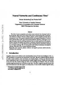
Fig. 1: Characteristics of hidden activations in adaptive and variational CTRNN layers: Since the timescale τ determines how activation is derived as an integration of previous activation yt−∆t and input x (see Eqn. 2), a larger variance σ leads to a different ratio between these, based on time step level sampling (dark grey: kept previous activation; white: input activation: light grey: uncertain ratio of both). The example shows m modules with increasing initial timescales. called AVCTRNN, we also introduce learnable weights s that steer the strength of the variance directly: t+τ0 τt = τAV +τσ t = 1+e

,

τσ ∼ N (0, s + σ0 )

. (5)

Fig. 1 illustrates how the adaptive and variational timescale characterise the hidden activations of a CTRNN layer. Larger t lead to stronger influence by previous activation and larger s to stronger variance on time step level. For comparison with the CTRNN, we can define the τ0 values in a way that parts of the layer group into modules because they share the same timescale. For example, such a layer with dense connectivity could have m = 3 modules with n = 100 neurons each, set to initial timescales 1, 2, and 4. Note, in this paper, such a module structure is considered horizontally only. Stacking layers vertically, as done in the aforementioned MTRNNs in order to impose hierarchical composition/decomposition, is possible and opens up further future studies. Since the new network parameters t and s are fully differentiable1 , we can train them together with the weights and biases in any end-to-end training fashion2 , but need to make sure to clip the values of τ in [1, ∞]. From the formal description (Eqn. 3–5), we can see that there is no actual need for specifying τ0 and σ0 and thus the notion of modules in the case of ACTRNNs and AVCTRNNs. However, this might be sensible for practical reasons, such as cutting training time because of a priori knowledge about the task or keeping the networks more comparable to the baseline, e.g. when comparing pre-determined initial timescales.

(3)

,

f(z,m)

...

... sampling

where the exponential function ensures timescales in [1, ∞], and the vector τ0 can be defined as sensible initial values for the timescales in case of the weights t getting initialised around zero. We call a model, using this adaptive timescale, an ACTRNN. Second, the timescales are sampled from a Gaussian normal distribution N based on given mean τ0 and a vector of variance values σ0 = [0 . . . τ02−1 ]: τt = τV t ∼ N (τ0 , σ0 )

...

f(z,k) τ>1

internal states z

, (2)

for inputs x, previous internal states zt−∆t , weights W and V, bias b, and an activation function f . The timescale can be a pre-determined common parameter τ for all units or a vector τ of individual constants. In tasks with discrete numbers of time steps, the CTRNN can get employed as a discrete model, e.g. by setting ∆t = 1. Although we can derive the CTRNN from the leaky integrate-and-fire model and thus from a simplification of the Hodgkin-Huxley model from 1952, the network architecture was suggested independently by Hopfield and Tank in 1986 as a nonlinear graded-response neural network and by Doya and Yoshizawa in 1989 as an adaptive neural oscillator [15], [16]. Overall, the CTRNN can be understood as a generalisation of the Hopfield Network [17] with continuous firing rates and arbitrary leakage in terms of time constants. More specifically, compared to the Simple Recurrent Network (SRN, or Elman Network), the timescale τ (or τ) is an additional hyperparameter of asymptotically not leaking, thus a neuron might maintain part of its information for a longer time. This parameter provides an interesting mechanism to capture sequential aspects on different timescales or periodicities and is particularly crucial for the hierarchical abstraction capability of the Multiple Timescale Recurrent Neural Network (MTRNNs [18]). In the MTRNN, however, the hyperparameter needs to be chosen carefully, based on a priori known temporal characteristics of the data, which is usually done in coarse approximation on layer or module level. In contrast, time constants in the brain are subjects to change during development and are hypothesised to be directly related to temporal structures [19]. In our model, we propose two novel mechanisms to obtain an adaptive and variational timescale for each neuron. First, the timescales are governed by learnable weights t that work like a bias on the timescale instead on the activation: t+τ0 τt = τA t =1+e

f(z,1)

activation

(1)

∆t (Wx + Vyt−∆t + b) τ

...

outputs y

(4)

1 Note,

s defines the range of the sampling but not the sampling itself. we can use any deterministic method, such as gradient descent (or arbitrary accelerated, adaptive, and regularising methods), based on suitable representations for the task as well as transfer and respective error functions.

where τ0 is a hyperparameter, set before training. Models using this variational mechanism are called VCTRNN henceforth. In order to finally combine both mechanisms in a model

2 Here,

14

III. E VALUATION AND R ESULTS In order to study our adaptive and variational timescale mechanisms, we ran tests on small baseline and more complex real-world tasks for both classification and prediction. The most interesting insight beyond the effect of the dynamic timescales in terms of performance is the adaptation and variation itself. In all tasks, we compared the ACTRNN, VCTRNN, and AVCTRNN variants against the CTRNN baseline as well as the SRN and the Long-Short Term Memory (LSTM [20]). For all setups, the hyperparameters have been optimised independently along learning parameters and methods, numbers and sizes of modules, and initial or fixed timescales (CTRNN case), but deliberately training in unregularised fashions3 . Our initial hypothesis was that the novel CTRNN variants will perform at least equal to a perfectly optimised CTRNN, without the need of optimising the timescales in hyperparameter space, significantly better than the SRN, and on par with the LSTM.

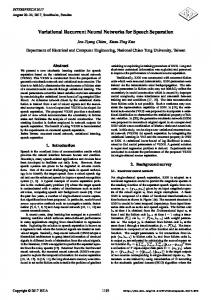
Fig. 2: Predicted sine waves versus targets of different periods. Vertical bar indicates first time step of closed loop prediction.

A. Experiment 1: Sequential MNIST Classification In the first task, we compared all networks on the sequential MNIST test for classification. We found accuracy results as presented in TABLE I, showing that the task can get easily solved by all networks and that the novel CTRNN variants perform equally: neither significantly better nor worse than the baseline. The best networks comprised a hidden layer partitioned into four modules with timescales (1, 3, 9, 27). TABLE I: Test accuracy for seq. MNIST classification (in %). SRN

CTRNN

ACTRNN

VCTRNN

AVCTRNN

LSTM

96.34

97.17

97.77

97.48

97.96

98.83

(a) ACTRNN: τ during training.

(b) Final τ CDF.

(c) AVCTRNN: σ during training.

(d) Final σ CDF.

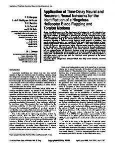
Fig. 3: Timescale τ development (top) and variance σ development (bottom) in the sine wave prediction task: adaptation during training (left) and distribution after training (right).

B. Experiment 2: Synthetic Sine Wave Prediction Function (CDF) form for comparing the adaptive CTRNN variants in Fig. 3a–b. This shows that in the ACTRNN, timescales are mostly kept around values that work best for the baseline CTRNN, but also small deviations around these attractors are developed. The variance σ in the AVCTRNN (Fig. 3c–d) surprisingly develops on a rather small scale, as for neurons with a small timescale, a tiny variance emerges in the first epoch, but nearly vanishes during training, while the variance for neurons with larger timescales also changes only slightly. This indicates that for such a simple task, the network does not learn, whether noisy activations facilitate or disturb the prediction.

In this second task, we were interested in how the CTRNN variants can capture the periodicities of some simple sine waves, instead of just remembering a whole set of sequences. Thus, we defined five training and three complementary test sines as a summation of sines with four different periods π/0.25, π/0.5, π/1.0, and π/4.0 over a course of 200 time steps. For the test sequences, the networks only see the first 50 time steps as an input and receive for the remainder their output prediction in a closed loop instead. The resulting predictions are presented in Fig. 2 for all networks. All networks can easily learn the regularities of sines with different periods and show only consistent minor shortcomings in fitting short periods perfectly. Thus, overall the CTRNN variants can solve this task equally well for the optimised cases with module sizes of (32, 16, 8, 4) and timescales4 around (1, 3, 9, 27). The development of the adaptive timescales is presented epoch-wise for the ACTRNN and in Cumulative Distribution

C. Experiment 3: Human Motion Patterns Prediction With the third task, we aimed at investigating how the CTRNN variants learn to capture the probabilistic periodic fluctuations in human-generated hand motion sequences. These motion sequences have been recorded as concatenations of three prototypical patterns (each standing for a symbol A, B, or C) during the study on VBP-RNN by Ahmadi and Tani [11]. Over 400 time steps, these symbols repeat with differing period lengths and form reoccurring word-like patterns.

3 All particularly interesting hyperparameters are included in the following sections, while the reference implementations are available on GitHub: https://github.com/heinrichst/ACTRNN . 4 Note: The timescales relate to the periods, with respect to timesteps in the sequence, and are only fixed for the CTRNN and VCTRNN.

15

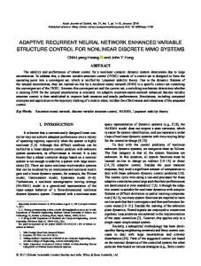
Since the test data contains complementary combinations of the symbols, the networks must be able to learn patterns on both short and long timescales. All predictions and the target patterns for the first sequence of the test data (closed loop from time step 200 onwards) are presented in Fig. 5a. Predicting the correct pattern fluctuations for time steps 230 onwards is rather difficult because no information of this pattern combination is given in the training data or via the initial state of the network. Thus, we observe how the SRN (and to some degree also the LSTM) seems to repeat oscillations with periods that it has often seen during training, while the CTRNN variants try to predict the most plausible symbol-fluctuation pattern (in this sequence inaccurate, but in itself correct). The Network with the adaptive timescale (ACTRNN) is additionally more precise in predicting the short periods, which indicates that it is better tuned to these fluctuations as well. However, the network with the fixed variations (VCTRNN) predicts with more extreme deviations in the case of a perturbing pattern around step 250, indicating that it might have forgotten some longer-term dependencies between the patterns that represent our symbols. From the hidden activations in Fig. 5b, we can obtain that neurons with smaller timescales, but at the same time nearly zero variance, show highly dynamic activations during these time steps, while neurons with larger timescales change from continuous activation to shorter bursts. From the development of the adaptive timescales as presented in Fig. 4, we can confirm our previous observations. For this more difficult task, which nevertheless shows rhythmic patterns, we can find timescales in the ACTRNN that are similar to the values of the best tuned CTRNN (in this case with (1, 5, 25, 125)), with notable deviations of larger timescales. The variance σ, however, has seemingly dropped for smaller timescales and only stayed high for larger ones. Overall, this indicates that it might be beneficial to adapt individual neurons in leaking less or stronger, but that variances in timescales seem to be difficult to handle by the network.

(a) ACTRNN: τ during training.

(b) Final τ CDF.

(c) AVCTRNN: σ during training.

(d) Final σ CDF.

(a) Plots of predicted patterns (targets in black and grey).

(b) Hidden activation (top: ACTRNN, bottom: AVCTRNN).

Fig. 5: Representative plot of predicted motion patterns sequence versus the target and corresponding hidden activation in relation to timescales τ or variance σ over 60 hidden units.

Fig. 4: Timescale τ development (top) and variance σ development (bottom) in the motion patterns prediction task.

16

timescales, however, remain active for longer times but also change activation rapidly when the meaning of the sentence gets drastically ambiguous, for example, if a subordinate clause starts or ends (for instances in step 13 and 26). It seems that the slow units of the network learn to contribute longer time dependency and by this modulate the faster units. When comparing ACTRNN and AVCTRNN, we cannot identify remarkable differences between activations sorted by timescale or sorted by variance σ. On the contrary, similar to our observations in the previous task, high timescales seem to correlate strongly with higher variance values, which appear to contribute little to changes in the modulation of faster units. In tracing the hidden activation correlated to timescale values (see Fig. 6) we can confirm that faster units activate chaotically while slower units show continuous activation patterns for shorter and longer parts of the sequence. Although these traces are already visible in the CTRNN, activations in the ACTRNN self-organise during development to quite different patterns. Units on timescale τ = 1 fluctuate constantly, are activated sporadically on timescale 2–3, and remain active on timescale 6–10 for specific parts of the sequence. In the test data, sentences usually have on average 20 words, but since many sentences contain embedded clauses, the semantically dependent phrases are on average 8 words long. Thus, comparing our observations with the data, it seems plausible that slower units learn the semantics of these clauses, while the units on timescales 2–3 perhaps capture shorter N -grams.

TABLE II: Test perplexity (PPL) on Penn TreeBank. SRN 118.30

CTRNN ACTRNN VCTRNN AVCTRNN LSTM 113.61

113.02

113.60

113.26

116.61

D. Experiment 4: Penn TreeBank Language Modelling For the fourth task, we evaluated how the networks perform on a small but well-known real-world task: language modelling on the Penn TreeBank corpus. Here, we were interested in how the CTRNN variants are reflecting the short-term dependencies (next words) or long-term dependencies (clause semantics) of the data. We focused on the most common setup, having 82K tokens of test data, a vocabulary size of 10k, using hidden layers of small size (in our case around 1400 neurons, leading to < 2M parameters), and training unregularised [21]. The word-level test perplexity is presented in TABLE II, indicating comparable results between the CTRNN variants (timescales: (1, 2, 4, 8)) and significant improvements over the basic LSTM (fair hyperparameter search, no peepholes) and the SRN. From inspecting the hidden activation during a test run on a word sequence (see Fig. 7) we can learn that units with small timescales activate with strong dynamics and small sparsity, supposedly to activate word vectors. Units with higher

Fig. 6: Hidden activation in relation to timescales τ or variances σ for the PTB task on the first 35 test data words over 1,300 hidden units: ACTRNN (top) and AVCTRNN (bottom).

Fig. 7: Traces of hidden activation with respect to the developed timescales τ on the first 35 words of the Penn TreeBank task: CTRNN (top) and ACTRNN (bottom).

17

IV. D ISCUSSION Timescales in recurrent networks can be modelled to be adaptive and variational. Based on fully differentiable dynamic modifications, an adaptive and variational CTRNN can tune the timescales automatically during development towards the long-term and short-term characteristics underlying the data. In our tests, this was particularly visible for more difficult tasks that nevertheless show rhythmic patterns on certain timescales, where we need to tune a baseline CTRNN to timescales using expert knowledge and intensive hyperparameter optimisation. In sequence prediction tasks such as for motion, the ACTRNN and AVCTRNN networks converged to similar timescale settings but were able to cope with subtle differences in fluctuations better by developing functional nodes that contribute with slightly different leakage of information and thus different periodicity. Classification tasks like language modelling revealed that our CTRNN variants, in fact, can self-organise their temporal sensitivity so that a developed network activates a broad range of differently slow temporal dynamic nodes in conjunction with many fast-forgetting nodes. This indicates that a tight coupling of nodes which mainly modulate activity and nodes which encode perceptual characteristics might be a natural result of mechanisms such as our proposed adaptation. To our surprise, however, positive effects of variations – or noise – on timescale level were evident rather for classification tasks only, while positive effects of adaptive but deterministic timescales were mostly visible in prediction tasks. A limitation of our approach could be the focus on deterministic error functions, instead of including a true variational inference by means of maximising the evidence lower bound of temporal fluctuations as it is done in VAEs or VBP-RNNs [11], [22]. Further studies, therefore, could explore our mechanisms in setups that include modelling a variational component, which adopts chaotic perturbations, as well. Overall, nevertheless, compared to other successful recent mechanisms from machine learning [12]–[14], automatically tuning the timescales is achieved in our approach by a comparably simple modification of the generally bio-plausible CTRNN. In our view, this allows for a range of interesting studies within the developmental robotics community, particularly towards investigating embodied language processing [8], [9]. As a first example, this includes hierarchical abstraction from temporally dynamic natural observations such as motion patterns or audio information, where the differing timescales carry structuring information. A second example concerns multi-modal integration and representation formation in human-robot interaction scenarios, where streams on different timescales contain complementary sensorimotor information about common aspects or events. By these means, we can further elaborate representation formation and functional aspects of timescale dynamics as well as activity coupling in both simulation and robotic real-word experiments.

R EFERENCES [1] D. Amodei, S. Ananthanarayanan, R. Anubhai, J. Bai, E. Battenberg, C. Case, J. Casper, B. Catanzaro, Q. Cheng, G. Chen et al., “Deep speech 2: End-to-end speech recognition in English and Mandarin,” in Proc. International Conference on Machine Learning (ICML), 2016, pp. 173–182. [2] A. Bordes, Y.-L. Boureau, and J. Weston, “Learning end-to-end goaloriented dialog,” in Proc. International Conference on Learning Representations (ICLR), 2017. [3] J. Koutnik, K. Greff, F. Gomez, and J. Schmidhuber, “A clockwork RNN,” in Proc. International Conference on Machine Learning (ICML), 2014, pp. 1863–1871. [4] K. Cho, B. Van Merri¨enboer, C. Gulcehre, D. Bahdanau, F. Bougares, H. Schwenk, and Y. Bengio, “Learning phrase representations using rnn encoder-decoder for statistical machine translation,” in Proc. Conference on Empirical Methods in Natural Language Processing (EMNLP), 2014, pp. 1724–1734. [5] G. Buzs´aki and A. Draguhn, “Neuronal oscillations in cortical networks,” Science, vol. 304, no. 5679, pp. 1926–1929, 2004. [6] D. Badre, A. S. Kayser, and M. D’Esposito, “Frontal cortex and the discovery of abstract action rules,” Neuron, vol. 66, no. 2, pp. 315–326, 2010. [7] A. K. Engel, C. Gerloff, C. C. Hilgetag, and G. Nolte, “Intrinsic coupling modes: multiscale interactions in ongoing brain activity,” Neuron, vol. 80, no. 4, pp. 867–886, 2013. [8] A. Cangelosi and T. Ogata, “Speech and language in humanoid robots,” Humanoid Robotics: A Reference, pp. 1–32, 2016. [9] S. Heinrich and S. Wermter, “Interactive natural language acquisition in a multi-modal recurrent neural architecture,” Connection Science, vol. 30, no. 1, pp. 99–133, 2018. [10] S. Murata, J. Namikawa, H. Arie, S. Sugano, and J. Tani, “Learning to reproduce fluctuating time series by inferring their time-dependent stochastic properties: Application in robot learning via tutoring,” IEEE Transactions on Autonomous Mental Development, vol. 5, no. 4, pp. 298–310, 2013. [11] A. Ahmadi and J. Tani, “Bridging the gap between probabilistic and deterministic models: a simulation study on a variational bayes predictive coding recurrent neural network model,” in Proc. Int. Conference on Neural Information Processing (ICONIP), 2017, pp. 760–769. [12] D. Neil, M. Pfeiffer, and S.-C. Liu, “Phased LSTM: Accelerating recurrent network training for long or event-based sequences,” in Proc. Advances in Neural Information Processing Systems (NIPS), 2016, pp. 3882–3890. [13] S. Chang, Y. Zhang, W. Han, M. Yu, X. Guo, W. Tan, X. Cui, M. Witbrock, M. A. Hasegawa-Johnson, and T. S. Huang, “Dilated recurrent neural networks,” in Proc. Advances in Neural Information Processing Systems (NIPS), 2017, pp. 76–86. [14] Y. B. Junyoung Chung, Sungjin Ahn, “Hierarchical multiscale recurrent neural networks,” in Proc. International Conference on Learning Representations (ICLR), 2017. [15] J. J. Hopfield and D. W. Tank, “Computing with neural circuits: A model,” Science, vol. 233, no. 4764, pp. 625–633, 1986. [16] K. Doya and S. Yoshizawa, “Adaptive neural oscillator using continuoustime back-propagation learning,” Neural Networks, vol. 2, no. 5, pp. 375–385, 1989. [17] J. J. Hopfield, “Neural networks and physical systems with emergent collective computational abilities,” Proceedings of the National Academy of Sciences of the United States of America, vol. 79, no. 8, pp. 2554– 2558, 1982. [18] Y. Yamashita and J. Tani, “Emergence of functional hierarchy in a multiple timescale neural network model: A humanoid robot experiment,” PLOS Computational Biology, vol. 4, no. 11, pp. 1–18, 2008. [19] B. J. He, “Scale-free brain activity: Past, present, and future,” Trends in Cognitive Sciences, vol. 18, no. 9, pp. 480–487, 2014. [20] K. Greff, R. K. Srivastava, J. Koutn´ık, B. R. Steunebrink, and J. Schmidhuber, “LSTM: A search space odyssey,” IEEE Transactions on Neural Networks and Learning Systems, vol. 28, no. 10, pp. 2222–2232, 2017. [21] T. Mikolov, “Statistical language models based on neural networks,” Ph.D. dissertation, Department of Computer Graphics and Multimedia, Brno University of Technology, Brno, CR, 2012. [22] D. P. Kingma and M. Welling, “Auto-encoding variational Bayes,” in Proc. International Conference on Learning Representation (ICLR), 2014.

ACKNOWLEDGMENT The authors thank Ahmadreza Ahmadi and Jun Tani for their effort in providing the human motion sequences data.

18