neural networks and adaptive computers

NEURAL NETWORKS AND ADAPTIVE COMPUTERS THEORY AND METHODS OF STOCHASTIC ADAPTIVE COMPUTATION

HUAIYU ZHU

University of Liverpool

Ph.D. Thesis

1993

Neural Networks and Adaptive Computers: Theory and Methods of Stochastic Adaptive Computation

Thesis submitted in accordance with the requirements of the University of Liverpool for the degree of Doctor in Philosophy by Huaiyu Zhu June 1993

Department of Statistics and Computational Mathematics University of Liverpool

NEURAL NETWORKS AND ADAPTIVE COMPUTERS: THEORY AND METHODS OF STOCHASTIC ADAPTIVE COMPUTATION HUAIYU ZHU

Abstract This thesis studies the theory of stochastic adaptive computation based on neural networks. A mathematical theory of computation is developed in the framework of information geometry, which generalises Turing machine (TM) computation in three aspects | It can be continuous, stochastic and adaptive | and retains the TM computation as a subclass called \data processing". The concepts of Boltzmann distribution, Gibbs sampler and simulated annealing are formally de ned and their interrelationships are studied. The concept of \trainable information processor" (TIP) | parameterised stochastic mapping with a rule to change the parameters | is introduced as an abstraction of neural network models. A mathematical theory of the class of homogeneous semilinear neural networks is developed, which includes most of the commonly studied NN models such as back propagation NN, Boltzmann machine and Hop eld net, and a general scheme is developed to classify the structures, dynamics and learning rules. All the previously known general learning rules are based on gradient following (GF), which are susceptible to local optima in weight space. Contrary to the widely held belief that this is rarely a problem in practice, numerical experiments show that for most nontrivial learning tasks GF learning never converges to a global optimum. To overcome the local optima, simulated annealing is introduced into the learning rule, so that the network retains adequate amount of \global search" in the learning process. Extensive numerical experiments con rm that the network always converges to a global optimum in the weight space. The resulting learning rule is also easier to be implemented and more biologically plausible than back propagation and Boltzmann machine learning rules: Only a scalar needs to be back-propagated for the whole network. Various connectionist models have been proposed in the literature for solving various instances of problems, without a general method by which their merits can be combined. Instead of proposing yet another model, we try to build a modular structure in which each module is basically a TIP. As an extension of simulated annealing to temporal problems, we generalise the theory of dynamic programming and Markov decision process to allow adaptive learning, resulting in a computational system called a \basic adaptive computer', which has the advantage over earlier reinforcement learning systems, such as Sutton's \Dyna", in that it can adapt in a combinatorial environment and still converge to a global optimum. The theories are developed with a universal normalisation scheme for all the learning parameters so that the learning system can be built without prior knowledge of the problems it is to solve.

Acknowledgements I would like to express my sincere thanks to Dr. R. Wait for his help and supervision during the preparation and writing of this thesis. Without his patient scrutiny of so many revised versions the pile of half-baked ideas which was to become this thesis would never become this thesis. I would also like to express my gratitude to the British Council, The State Educational Commission of China, and the Y. K. Pao Foundation, who co-sponsored this research through the Sino-British Friendship Scholarship Scheme (SBFSS). I want to thank Prof. J. G. Taylor of King's College London for inspiring communication and for introducing me to the literature of reinforcement learning. I am grateful to my wife for her understanding, encouragement and support during dicult times. A number of ideas in the thesis also initialised during our discussion. Thanks are also due to the sta in the Department of Statistics and Computational Mathematics for their assistance and advice, and my other friends and colleagues for their help and understanding while I was completing this thesis.

To My Parents and My Wife

Contents I Fundamentals 1 Introduction

1.1 Motivation : : : : : : : : : : : : : : : : : : : : : : : : : : : : : : : : : : : 1.2 Theoretical Framework : : : : : : : : : : : : : : : : : : : : : : : : : : : : : 1.3 Outline of the Thesis : : : : : : : : : : : : : : : : : : : : : : : : : : : : : :

1 2 2 3 8

2 Review of Related Work

11

3 Adaptive Information Processing

20

2.1 SCAP: Neural Networks : : : : : : : : : : : : : : : : : : : : : : : : : : : : 11 2.2 TCAP: Reinforcement Learning : : : : : : : : : : : : : : : : : : : : : : : : 14 2.3 Information Theory and Related Topics : : : : : : : : : : : : : : : : : : : 17 3.1 3.2 3.3 3.4 3.5 3.6

Introduction : : : : : : : : : : : : : : : : : : : : : : Review of Probability Theory : : : : : : : : : : : : Information Geometry : : : : : : : : : : : : : : : : Entropy and Simulated Annealing : : : : : : : : : Markov Chains and Parameterised Markov Chains Adjustable Information Processors : : : : : : : : :

II Neural Networks 4 Theory of H. S. Neural Networks 4.1 4.2 4.3 4.4 4.5 4.6

Introduction : : : : : : : : : : : : : De nitions and Basic Properties : Classi cations and Restrictions : : Duality between DC- and SQ-NN : Generality of FB-NN and Stability Learning Rules : : : : : : : : : : :

: : : : : :

: : : : : :

: : : : : :

: : : : : :

: : : : : :

5.1 5.2 5.3 5.4 5.5

: : : : : :

: : : : : :

: : : : : :

: : : : : :

: : : : : :

: : : : : :

: : : : : :

: : : : : :

: : : : : :

: : : : : :

: : : : : :

: : : : : :

: : : : : :

: : : : : :

: : : : : :

: : : : : :

: : : : : :

: : : : : :

: : : : : :

: : : : : :

: : : : : :

: : : : : :

: : : : : :

: : : : : :

: : : : : :

Introduction : : : : : : : : : : : : : : : : : : : : : : : : SQB-NN: Boltzmann Machine : : : : : : : : : : : : : : DCF-NN: Multilayer Perceptron : : : : : : : : : : : : DCB-NN: Continuous Hop eld Net and Others : : : : DCFB-NN: Generalization of DCF-NN and DCB-NN :

: : : : :

: : : : :

: : : : :

: : : : :

: : : : :

: : : : :

: : : : :

: : : : :

: : : : :

: : : : :

: : : : :

i

: : : : : :

: : : : : :

: : : : : :

5 Classical Models of H. S. Neural Networks

: : : : : :

: : : : : :

20 20 22 25 32 36

39 40

40 40 43 48 50 54

58

58 58 62 64 68

CONTENTS

ii

6 Theory of SQFB Neural Networks 6.1 6.2 6.3 6.4 6.5 6.6 6.7

Introduction : : : : : : : : : : : : : : : : : : : : : : : : : : : Structure and Dynamics : : : : : : : : : : : : : : : : : : : : Relations with Other Networks : : : : : : : : : : : : : : : : GF-ME Learning Rule : : : : : : : : : : : : : : : : : : : : : GF Learning Converge to Local Optimum in Weight Space Simulated Annealing Learning Rule : : : : : : : : : : : : : : Information-theoretical interpretation of SA learning rule :

7 Implementation of SQFB Neural Networks 7.1 7.2 7.3 7.4 7.5 7.6

Introduction : : : : : : : : : : : : : : : : : : : Simulation of Gibbs Samplers : : : : : : : : : Encoder Problems and Ideal Learning : : : : Speed of Averaging, Learning and Annealing Simulation Experiments : : : : : : : : : : : : Comparison with Results of Others : : : : : :

III Adaptive Computers 8 Adaptive Markov Decision Process 8.1 8.2 8.3 8.4 8.5 8.6

Introduction : : : : : : : : : : : : : : : : : : : The Mathematical Model : : : : : : : : : : : Utility Function and Value Function : : : : : Properties of Utility Function : : : : : : : : : Equilibrium Policy and Simulated Annealing Equilibrium Meta-States : : : : : : : : : : : :

9 Basic Adaptive Computers 9.1 9.2 9.3 9.4 9.5 9.6 9.7

: : : : : :

: : : : : :

Introduction : : : : : : : : : : : : : : : : : : : : General Description of BAC : : : : : : : : : : : Implementing the Decision Module by DC-NN Two Test Problems : : : : : : : : : : : : : : : : Scaling and Speed : : : : : : : : : : : : : : : : Set-up of Experiments : : : : : : : : : : : : : : Numerical Simulations : : : : : : : : : : : : : :

10 Conclusions, Discussions, and Suggestions

: : : : : :

: : : : : : : : : : : : :

: : : : : :

: : : : : : : : : : : : :

: : : : : :

: : : : : : : : : : : : :

: : : : : :

: : : : : : : : : : : : :

: : : : : :

: : : : : : : : : : : : :

: : : : : :

: : : : : : : : : : : : :

: : : : : :

: : : : : : : : : : : : :

: : : : : : :

: : : : : : :

: : : : : : :

: : : : : : :

: : : : : : :

: : : : : : :

: : : : : : :

: : : : : : :

: : : : : :

: : : : : :

: : : : : :

: : : : : :

: : : : : :

: : : : : :

: : : : : :

: : : : : :

: : : : : : : : : : : : :

: : : : : : : : : : : : :

: : : : : : : : : : : : :

: : : : : : : : : : : : :

: : : : : : : : : : : : :

: : : : : : : : : : : : :

: : : : : : : : : : : : :

: : : : : : : : : : : : :

10.1 Summary of Results : : : : : : : : : : : : : : : : : : : : : : : : : : : : : : 10.2 Open Questions and Future Work in Combinatorial Optimisation and Adaptive Information Processing : : : : : : : : : : : : : : : : : : : : : : : 10.3 Open Questions and Future Work in the Theory of Neural Networks : : : 10.4 Open Questions and Future Work in the Theory of Adaptive Computers : 10.5 Intelligence and Arti cial Intelligence : : : : : : : : : : : : : : : : : : : : : 10.6 Algorithms and Computations : : : : : : : : : : : : : : : : : : : : : : : : 10.7 Final Remarks : : : : : : : : : : : : : : : : : : : : : : : : : : : : : : : : :

70

70 70 72 73 76 80 82

92

92 92 95 100 129 131

135 136

136 136 140 142 144 150

154

154 154 156 157 159 165 165

174

174

175 176 178 181 185 187

CONTENTS

iii

A Preliminaries, Terminology and Notation A.1 A.2 A.3 A.4 A.5

General Terminology and Conventions Logic and Sets : : : : : : : : : : : : : Relations, Orders, Mappings : : : : : : Linear Algebra and Analysis : : : : : : Miscellaneous : : : : : : : : : : : : : :

B Glossary of Acronyms

: : : : :

: : : : :

: : : : :

: : : : :

: : : : :

: : : : :

: : : : :

: : : : :

: : : : :

: : : : :

: : : : :

: : : : :

: : : : :

: : : : :

: : : : :

: : : : :

: : : : :

: : : : :

: : : : :

: : : : :

189

189 189 190 193 195

198

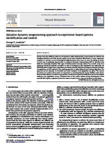
List of Figures 1.1 An adaptive computer (AC) constructed with trainable information processors (TIP) and xed information processors (FIP). : : : : : : : : : : : 1.2 One type of trainable information processor: simple-layered SQFB-NN. : 1.3 One layer of a SQFB-NN. : : : : : : : : : : : : : : : : : : : : : : : : : : : 1.4 A typical quasilinear neuron. : : : : : : : : : : : : : : : : : : : : : : : : : 4.1 4.2 4.3 4.4 6.1 6.2 6.3 6.4 6.5 6.6 6.7 7.1 7.2 7.3 7.4 7.5 7.6 7.7 7.8 7.9 7.10 7.11 7.12 7.13 7.14 7.15

Structure of an example neural network. : : : : : : : Two simple structures which are not strongly stable. Composition of two structures. : : : : : : : : : : : : A BF-NN composed of a B-NN and F-NN. : : : : :

:::::::::::: :::::::::::: :::::::::::: :::::::::::: Curves of hf i versus w for various and contours of hf i over w and on MW : : : : : : : : : : : : : : : : : : : : : : : : : : : : : : : : : : : : : : : 3D graphs of hf i versus and w on MW : : : : : : : : : : : : : : : : : : : Contour of hf i on M for four dierent , superimposed with the position of MW and w1 : : : : : : : : : : : : : : : : : : : : : : : : : : : : : : : : : 3D graphs of hf i on M for four dierent : : : : : : : : : : : : : : : : : : Learnt probability distributions p(i) at dierent for a three-neuron network with two randomly generated evaluation functions e(i) : : : : : : : : Learnt probability distributions p(i) at dierent for a four-neuron network with two randomly generated evaluation functions e(i) : : : : : : : : Learnt probability distributions p(i) at dierent for a ve-neuron network with two randomly generated evaluation functions e(i) : : : : : : : : Four examples of 4-4 encoder with constant speed (a) : : : : : : : : : : : Four examples of 4-4 encoder with constant speed (b) : : : : : : : : : : : Three examples of 4-4 encoder with scaled speed (a) : : : : : : : : : : : : Three examples of 4-4 encoder with scaled speed (b) : : : : : : : : : : : : Four examples of 4-2-4 encoder (a) : : : : : : : : : : : : : : : : : : : : : : Four examples of 4-2-4 encoder (b) : : : : : : : : : : : : : : : : : : : : : : Three examples of 8-3-8 encoder (a) : : : : : : : : : : : : : : : : : : : : : Three examples of 8-3-8 encoder (b) : : : : : : : : : : : : : : : : : : : : : Two runs with redundant hidden units (a) : : : : : : : : : : : : : : : : : : Two runs with redundant hidden units (b) : : : : : : : : : : : : : : : : : : Three runs for the 2-2-2-2 encoder problem (a) : : : : : : : : : : : : : : : Three runs for the 2-2-2-2 encoder problem (b) : : : : : : : : : : : : : : : Three examples of the three layer encoder problem (a) : : : : : : : : : : : Three examples of the three layer encoder problem (b) : : : : : : : : : : : Four examples of the 5-3-5(8) random code problem (a) : : : : : : : : : : iv

4 5 5 6 41 51 52 53 84 85 86 87 88 89 90 109 110 111 112 113 114 115 116 117 118 119 120 121 122 123

LIST OF FIGURES 7.16 Four examples of the 5-3-5(8) random code problem (b) : : : : : : : : : : 7.17 The ideal learning curve for the Hamming distance encoder and the encoders de ned in [AHS85] (a) : : : : : : : : : : : : : : : : : : : : : : : : : 7.18 The ideal learning curve for the Hamming distance encoder and the encoders de ned in [AHS85] (b) : : : : : : : : : : : : : : : : : : : : : : : : : 7.19 Four examples of the 4-2-4 encoder without simulated annealing (a) : : : 7.20 Four examples of the 4-2-4 encoder without simulated annealing (b) : : : 9.1 A neural network as a trainable information processor (TIP) : : : : : : : 9.2 The ideal learning curves for the counting game. : : : : : : : : : : : : : : 9.3 Normalised evaluation corresponding to equilibrium strategies of the counting game for mT 2 f7; 8; 9; 10g, n = 3 : : : : : : : : : : : : : : : : : 9.4 Normalised evaluation corresponding to equilibrium strategies of the counting game for mT 2 f46; : : :; 50g, n = 5 : : : : : : : : : : : : : : : : : 9.5 History of a typical trial of the \counting game" after 2000 trials in a typical run. : : : : : : : : : : : : : : : : : : : : : : : : : : : : : : : : : : : 9.6 Samples from the history of a run of BAC on the moving point game : : : 9.7 A \cross section" of the same run as Figure 9.6, after 4000 plays. : : : : : 9.8 Samples from the history of a run of BAC on the moving point game : : : 9.9 A \cross section" of the same run as Figure 9.8, after 2000 plays. : : : : :

v 124 125 126 127 128 155 161 162 163 167 169 170 171 172

A.1 Graphs of frequently used elementary functions. : : : : : : : : : : : : : : : 196

Part I

Fundamentals

1

Chapter 1

Introduction 1.1 Motivation It has long been a dream of people to design a machine which can think. The advent of computers had been the hope of many that this might become a reality. Much has been achieved by the computer sciences toward this goal, but the traditional symbolic arti cial intelligence failed in a crucial point: however smart a computer can be in doing many jobs, it does not behave like human beings. The most dicult problems for computers are just those problems which are most simple for humans, even for some other animals. Does this re ect some fundamental dierences between a machine and a conscious being? Or is this merely because the computers of today are not yet complicated enough? This is the core of the current intensive debate concerning the so-called \strong-AI thesis" [Sea80]. Although it is accepted common sense in the scienti c community that there is no mystic force behind the phenomenon of intelligence, it is evident that the current computational theory lacks something essential to account for it. This is even more remarkable considering that Turing machines (TM) are universal computational machines. Recent exciting developments in connectionist models of computation [RM86, MR86] point out two possible extensions to TM which seems to be essential for intelligence: the stochastic nature of general computation and the accumulation of information. Although these ideas were already present in Turing's rst account of arti cial intelligence [Tur50], they remained largely ignored in the later developments of computational science. In this thesis we try to develop a uni ed theory and general methods of stochastic adaptive computations based on neural networks (NN). The results suggest some new directions in which the debate on strong-AI thesis might be resolved, in science rather than philosophy. For the purpose of introduction, a brief recollection of the particular train of thought leading to this theory is probably more informative. The starting point is the backpropagation learning rule [RHW86] and the results that feedforward NNs are in a sense universal approximators of functions [Fun89, HSW89]. This means that NN can be regarded as a parameterised function which can adjust itself to suit the demand. The question I asked was: \Can such devices learn to play chess?" This question is quite legitimate since the rules of chess are well de ned. It is also signi cant since, as many pioneers of computational theory had recognised [Wie48, Tur50, Sha50, Tur53], if computers can learn to play games like chess, they can do things hitherto considered as the reserve of human intelligence. 2

CHAPTER 1. INTRODUCTION

3

One aspect of games like chess of particular importance to computational theory is that it is impossible to enumerate all the possibilities of the game, even with the resource of the universe [Sha50]. This makes it a necessity that any successful method for such problems be adaptive, or incremental, so that it can provide a solution with limited resources, and can improve the solution whenever more resources are available. What a human player knows about chess which makes him a good player even before he can actually enumerate all the possibilities? A human player of chess learns two basic things: how to evaluate each board position; and which move is likely to lead to good positions. The rst fundamental question arises: What does it means that a position is \good"? After a moment of re ection, one can be sure that the optimality of a position must be a measure monotonically related to the probability of winning. Since the rules of chess is deterministic, the players must play stochastically 1 . Here we restate our principal observations: First, for a system to be intelligent, it must be able to learn more than what it is programmed for; and second, in order for the concept of learning to be well de ned in this sense, the system itself must act stochastically, independently of whether the environment is stochastic. Assuming that the players use stochastic strategies, a learning machine for playing chess can, at least in principle, be constructed with two NNs, one for evaluation of board positions and the other for producing the moves stochastically. It is obvious, however, that there is nothing special to chess in this formulation: the learning machine thus constructed would seem to incorporate all the ability of human problem solving in an \arbitrary" environment. How far this approach can go in the direction of building a general problem solving machine can only be decided by quantitative studies, of which this thesis is intended to be a rst step. As is evident from the above discussion, our concept of \computation" is extended from that based on the formal de nition of TMs. To avoid discussions which go too far a eld in this introduction, we simply call our new concept \stochastic adaptive computation" while the classical one as \TM computation". We return to motivation in the conclusions in x10.5.

1.2 Theoretical Framework As soon as one tries to build a theory of \intelligent behaviour" based on so-called \mechanical elements", one realizes that there is a vast level of complexity. The complexity of a theory does not depend on what it studies, but on the \distance" between its overall structure and its fundamental building blocks. We call this the scope of complexity. The most ambitious objective along the direction outlined above seems to be to account for the intelligent behaviour of an animal in complex environments based on the details of neurons in its brain. In this thesis we focus our attention on the more realistic scope of complexity: down to some regular and mathematically well de ned neurons, up to the discrete time decision The reason for stochastic behaviour in chess-playing is dierent from traditional situations where there are stochastic elements in the environment: If the two players are assumed to be of similar mentality, neither player can be less stochastic than his environment, which consists of the other player and the deterministic rules. The degree of stochasticity can be measured, for example, by the entropy of the action selection process. 1


4

problems in some Markovian environments 2 . Even this is too complex, so the theory is divided into two levels: the theory of \adjustable information processors" and the theory of \adaptive computers". The former takes into account the lower part of the scope of complexity, while the latter the upper part. This framework is illustrated schematically in the series of four \zoom in" gures, Figure 1.1{1.4, where each succeeding gure details part of its predecessor. We shall return to these gures in the reversed order in the main body of the thesis. (Figure 1.4 in x4.2, Figure 1.2 & 1.3 in x4.3, and Figure 1.1 in Chapter 9.)

Figure 1.1: An adaptive computer (AC) constructed with trainable information processors (TIP) and xed information processors (FIP).

x(t){input, y(t){output and r(t){reward. The concept of AIP is an abstraction of the TMs and a subset of NNs (all those to be studied here). The former is called a programmable information processor (PIP) and the latter a trainable information processor (TIP). Each AIP realizes a (stochastic) mapping from its input to its output depending on some parameters (abstraction of programs or connection weights) which can be adjusted to increase the expectation of immediate evaluation of the input-output pair. Whether this is done arti cially (by some outside programmer) or automatically (by AIP itself) dierentiates between PIP and TIP. A physical device implementing a xed (stochastic) mapping is called a xed information processor (FIP), which is equivalent to a communication channel [Sha48] although with quite dierent purposes. A PIP with a given program is a deterministic FIP. The concept of AC is an abstraction of animal brains and arti cial adaptive computational devices. An AC works in a certain, but quite arbitrary environment, receiving a time sequence of inputs, emitting a time sequence of outputs, receiving a time sequence of rewards in return, and modifying internal parameters so as to increase the utility of each state, which is the expectation of a particular form of accumulated reward it would receive in the future following that state. If an AC can be modelled by a Markov decision process (MDP), it is called a basic adaptive computer (BAC). In the concluding chapter we shall make some suggestions on how the top line might be raised to include more complex environments. 2


5

Figure 1.2: One type of trainable information processor: simple-layered SQFB-NN.

x{input, y{output, e{evaluation.

Figure 1.3: One layer of a SQFB-NN. Each circle is a neuron. Note that there are bidirectional connections inside each layer, and unidirectional connections between layers.


6

Both TIP and AC are systems which accumulate information while processing it. What dierentiates TIP and AC is that for the former the adjustment of the parameter only depends on the evaluation of the input-output pairing. It does not depends on how the past might in uence the present, nor how the present might in uence the future. Nor does it take into account that the environment might change in response to its own change.

Figure 1.4: A typical quasilinear neuron. The input is linearly combined (), and nonlinearly transformed (f ). The output is broadcast to other neurons along connections. In biological analogy, the big circle is the soma, the semi-circles to the left are synapses, the semi-circle to the right is the axon, and the arrowed lines are dendrite. * * * The distinction between adjustable information processor (AIP) and adaptive computer (AC) is one of the most important feature in the structural framework of our theory. The basic idea behind this is that AC can be constructed from modules each composed of a TIP and some FIP. As a metaphor, we consider TIP and FIP as standard components and the AC as a complete machine. Neural networks t in this picture as certain \universal" TIPs. When we study NNs, we only consider what it is required as a TIP; when we study ACs, we take for granted that there are TIPs for implementing required stochastic mappings. The signi cance of such a \division of labour" can be somehow explained through the concept of credit assignment problem (CAP) for learning machines [Min61], although we shall seldom have chance to mention this concept in technical discussions. The study of TIPs corresponds to the so-called structural credit assignment problem (SCAP), where given an evaluation of a system, it is required to assign the credit proportionately to various subsystems. The study of ACs corresponds to the so-called temporal credit assignment problem (TCAP), where given the evaluation of a mission, ie., a sequence of decisions, it is required to assign the credit proportionately to various steps in its execution. There is also a biological analogy: the study of TIPs and ACs correspond respectively to neurological and behavioural studies. Our theoretical framework puts strong constraints on both TIPs and ACs: The TIPs must be able to be connected in a modular structure; It is not enough that NNs are designed as independent models, as is being done in most NN research nowadays. The ACs must be stable; this cannot be derived simply from the fact that all its components are stable in a stationary environment. Considerations of such kind will sometimes be explicitly stated, but mostly implicitly applied throughout the thesis.


7

* * * We try to provide both the mathematical theory and computational methods, the latter having further requirements. Our goal is to see how much of the constructions of pure mathematics can be carried out by physical devices restricted in the universe . Considering that there are only about 1010 neurons in the human brain [And83] and about 1080 atoms in the whole observable universe [Dav82], the following concepts, closely related to the concept of NP-completeness [GJ79], are very important for comparing the computational viability of various theories. A nite set X is said enumerable 3 if, by a proper coding method, all of its elements can be examined, either simultaneously, or sequentially over a tolerable duration of time, in a physical device of current technology. A set X is combinatorially enumerable if its elements can be labelled by a coding system An , where A is the alphabet, n is the maximum length of code, such that nA := f(k; a) : k 2 Nn; a 2 Ag is enumerable. If X is (combinatorially) enumerable, we also100say that jX j, the number of members of X , is so. For example, sets of 100, 2100 and 22 elements are enumerable, not enumerable but combinatorially enumerable, and not combinatorially enumerable, respectively 4 . A combinatorial optimisation problem is a global optimisation problem over a combinatorially enumerable set. By de nition, only approximate solutions are in general achievable. To date, the most ecient general methods to combinatorial optimisation problems are stochastic methods, such as simulated annealing (SA) method and genetic algorithms (GA). This is no coincidence, and its root can only be explained by the information theory. Classical computational theories have always been theories of certainties, in which the structure \if : : : then : : : else : : : " takes care of all the imaginable possibilities. As soon as we are faced with problems for which it is even impossible to imagine all the possibilities before they actually occur, the amount of information in a problem becomes more important than the amount of data . The value of these two measures diverges as the probability distribution becomes less uniform. The stochastic methods have the ability to process an enumerable amount of information embodied in a combinatorially enumerable amount of data, by dealing with some parts of the data with diminishing, but still positive, probability. There are at least two other reasons why stochastic computations are important for intelligence: (1) The environment might be stochastic; (2) In game theory, the optimal strategy may exist only if mixed strategies are allowed 5 . In these two \classical" reasons: either the condition or the solution of a problem is stochastic. However, as we have just seen, facing with combinatorial problems, even if the condition and the optimal solution are both deterministic, it may still be necessary to use a stochastic method. One of the mathematical foundations of stochastic computation is the theory of Markov chains (MCs). Since in our theory the computation is also adaptive, so that the MC itself will also move as learning proceeds, we must consider the space of all the MCs. Fortunately, the fundamental concepts for such consideration have already been 3 This has nothing to do with the concept of countable, sometimes also called denumerable, in set theory. 4 Although these concepts depend on the \current technology", these statements in this example have an absolute meaning if physical constraints are taken into account. The number 2100 1030 is more than 100 times larger than the total number of neurons in the brains of all the humans ever lived. 5 The terms \policy" and \strategy" are used interchangeably. Same applies to \stochastic policy" and \mixed strategy".


8

provided by the theory of information geometry (IG), which is the study of manifolds of probability distributions[AH89, AKN92]. * * * Our main purpose of studying NN is to develop more powerful computational devices. Therefore we shall mainly examine them from mathematical, and sometimes engineering, points of view. These \arti cial neural networks" (ANNs) are systems that we can control their internal construction. On the other side of the same coin are the \biological neural networks" (BNNs), which we know work very well, but we do not know how. Although the study of both ANNs and BNNs may be bene cial to each other in several ways, our theory does not logically depend on the study of BNNs. Numerous neural network models have appeared in the literature. It is impossible to de ne NN in such a way as to include everything which has been called NN without including something de nitely not to be called NN. We shall give formal de nitions for what we call the class of quasilinear neural networks (Q.NN). Our theory is further restricted to a subset of Q.NN, the class of homogeneous semilinear neural networks (H.S.NN). This restriction is justi ed by the following three simple reasons: the class of H.S.NN includes many of the most popular neural networks; it is general enough as a class of TIPs; and it is regular enough to allow a complete mathematical theory. Intuitively, the term \semilinear" means the input of each neuron is a linear combination of the inputs to the network and the outputs of all the other neurons. The term \homogeneous" means that the output of each neuron depends on the input of that neuron by a rule which is the same for all the neurons in the network.

1.3 Outline of the Thesis The next two chapters, Chapter 2 and Chapter A provide background material. Chapter 3 sets up the basic theoretical framework of this thesis. In the following four chapters, Chapters 4{7, we study neural networks as realizations of trainable information processors (TIPs), which solve the structural credit assignment problem. In Chapters 8 and 9, the concept of time is introduced into the problem. We study adaptive computers, which solve temporal credit assignment problem, provided that TIPs are available. Chapter 10 summarises the results, discusses various implications, and suggests future research directions.

Chapter 2: Related work to this research are reviewed. The emphasis is on the most signi cant and general related results, and no attempt is made at sorting out the rst contributor. There is no need to know anything about biology, engineering, or physics in order to logically follow this thesis, but a background in related elds would certainly help in comprehending the reason behind each development. The review is divided into three parts. In x2.1, various of neural networks are reviewed from the computational point of view. That is, we are mainly concerned with the most simple structures which can perform general tasks, instead of those models which are most descriptive of BNN. In x2.2, we review work related to our adaptive computers. An emphasis is on work which is most related to Markov decision processes (MDPs) (Chapter 8) and basic adaptive computers (BACs) (Chapter 9).


9

In x2.3, we review work related to our approach to stochastic adaptive computation. In particular, we review the related subjects in the following elds: probability theory, information theory, statistical mechanics, combinatorial optimisation (computational complexity, simulated annealing and genetic algorithms)

Chapter 3: We develop a mathematical theory of adaptive information processing in

general, based on probability theory and the theory of information geometry (IG). We shall formulate the entropy principle, which generalises the well-known maximum entropy principle, and show its relation with the simulated annealing (SA) method. We shall also apply the entropy principle to parameterised MCs, which forms the basis of the later chapters. The concept of trainable information processor (TIP) is also de ned in this chapter, which serves as an interface between NNs and ACs: each NN is a system whose functionality is a TIP, while an AC is a system whose main components are TIPs.

Chapter 4: We develop a mathematical theory of homogeneous semilinear neural net-

works (H.S.NN). The basic de nitions of structure and dynamics of quasilinear neural networks (Q.NN) are give in x4.2, and a classi cation is given in x4.3. In the rest of the thesis we focus on to a smaller class, H.S.NN, which from there on is also abbreviated as NN when there is no danger of confusion. The pre x notations S- (stochastic), D- (deterministic), C- (continuous), Q- (quantised, or discrete), F- (feedforward, multilayer, or associative), B- (feedback, symmetric connection, or correlative) are used to denote the classi cation of Q.NN. As listed in x4.3.4, the class of Q.NN includes some of the most well-known NNs. The intrinsic relations between SQ-NN and DC-NN are also discussed (x4.4). We also study the FBstructure which generalises F- and B- structures (x4.5). In x4.6 we give a general de nition of neural network learning rules. Various existing learning rules are studied and generalised. In particular, we shall show that most existing gradient-following (GF) learning rules can be transformed into simulated annealing (SA) learning rules, thus avoiding convergence to local optima in the learning process.

Chapter 5: We study some of the most important special examples of H.S.NN, including the DCF-NN (back-propagation network), the DCB-NN (Hop eld net), the SQF-NN (belief network) and the SQB-NN (Boltzmann machine). We shall also study DCFB-NN as a generalisation of DCF-NN and DCB-NN. Chapter 6: We develop the mathematical theory of SQFB-NN. The main thrust of this

chapter is the derivation of the learning rules, based both on GF and SA. A numerical example is provided in which GF learning rule inevitably leads to local optima. This is overcome by the SA learning rule. Our mathematical derivation of the learning rules reveals the reason behind and shortcomings of the so-called \Hebbian learning" mechanism, which have been used extensively ad hoc in many existing learning rules.

Chapter 7: We study various aspects concerning the implementation of SQFB-NN.


10

The core of a stochastic neural network is a Gibbs sampler (GS) (de ned in x3.4.1), which is also widely used in other stochastic computations. In x7.2 we derive a very ecient implementation of GS on a conventional computer, whose application should not be restricted to neural networks. In x7.3.3, we analyse a typical, and yet tractable example, the encoder problem, to derive theoretical relations between various parameters of learning and the performance of the network. We give a mathematical treatment of learning which has quantitative theoretical predictions subject to comparison with experiments. These theoretical results can only be understood in the sense of information theory, and are, to our best knowledge, completely new. Many numerical tests are performed for the SQFB-NN with the SA learning rule. In x7.5 we present and analyse the results concerning various aspects of learning. This is also compared with the Boltzmann machine (BM) learning rules. In fact, we shall show that there are actually two brands of BM learning rules, one corresponds to GF and the other to SA.

Chapter 8: We develop a mathematical theory of Markov decision process (MDP), which generalises the classical theory of dynamic programming (DP) and controlled Markov chains. Our generalisation is that the entropy principle (x3.4) in applied to the decision module (policy function in DP), so that the resulting learning rule is a multistage variant of simulated annealing which avoids local optima. This is necessary for implementing the MDP on neural networks. In our formulation many dierent problems in DP are treated in exactly the same way (x8.5.3). Chapter 9: We study how to implement the basic adaptive computer (BAC) based

on NN. Many possible variations to the main algorithm are given. Simulation results on two test problems are given in x9.7, one is a game of con ict of two players, where the solution contains many alternating regions of local optima. We show that it never converges to a global optimum if GF learning rules are used, and that it always converges to a global optimum if SA learning rules are used. Another problem reported in the same section also contains local optima. It also has an enormous state space. As far as we know, such solutions have never been reported before. In x9.5, we derive a normalisation convention which is universally applicable to BACs. Since it is dicult to get an exact theoretical result, we adopt a variant of the convention in x7.3.3. With this normalisation convention, we use the same program with same parameters to learn the two very dierent games.

Chapter 10: We summarise our results. We also further discuss the implications of this

research on various related research elds: arti cial intelligence, computer architecture, neural physiology and behavioural sciences, probability theory and information theory. We also comment on further researches in these directions, as well as on neural network theory and adaptive computer theory.

Appendix A: There are quite a few new notations introduced in this thesis. They are described in this appendix, together with a review of prerequisite mathematics.

Appendix B: This appendix lists explanation of all the acronyms used in the thesis.

Chapter 2

Review of Related Work The general problem we are going to study is stochastic adaptive computation in a certain general environment. Related work can be roughly divided into three classes: methods for solving structural credit assignment problems (SCAPs), methods for solving temporal credit assignment problems (TCAPs), and fundamental theory concerning general credit assignment problems for stochastic adaptive computation. Those pertaining to SCAPs include various neural networks and their learning rules. Those pertaining to TCAPs include game theory, the theory of dynamic programming, and various reinforcement learning methods. The fundamental theory pertaining to general credit assignment problem include theories on stochastic information processing, Markov chains and information geometry. We shall review only references which we consider to be landmarks in the development of the theory, excluding numerous special methods which may be very useful to speci c problems in practice but which do not feature in our general theory. Many similar concepts have been given various names in various research elds over the years. We shall give precise de nitions of the terms used in the thesis, we shall not attempt to mention the dierent and often con icting de nitions in the literature.

2.1 SCAP: Neural Networks Neural networks are also called connectionist models or parallel distributed processing (PDP) models. The reference book [Was90] includes over 4000 entries up to 1989, where 1988 alone counts for more than 1000. As we consider neural networks as physical realizations of trainable information processors (TIPs), our theory will be focussed on the class of homogeneous semilinear neural networks (H.S.NN), with supervised or reinforcement learning rules (these terms were brie y explained in x1.3, and will be de ned fully in Chapter 4) 1 . * * * There are generally three aspects of neural networks which are of mathematical interest: the structure, the dynamics and the learning rules. 1 This choice is based on the conviction that on the one hand H.S.NN form a quite general and rich subset of TIPs, and on the other they have handy physical interpretations. While the latter property does not guarantee more applications or easier manufacturing, it does make it much easier to obtain deep theoretical results necessary for analysis, design and application of neural networks, especially when several neural networks are to be connected together in a complex system.

11

CHAPTER 2. REVIEW OF RELATED WORK

12

The rst formal theory of neural network structures and dynamics is usually attributed to [MP43, PM47], where it was shown that the DQF-NN (deterministic quantised feedforward neural network) can implement any logical calculations, provided that there are enough neurons and the connection weights are right. The rst NN learning rule is usually attributed to [Heb49, p.62]. The rst formal theory on a type of arti cial neural networks with a learning rule is usually traced to [Ros58, Ros59], where a perceptron network is actually one layer of DQF-NN preceded by a layer of xed processors [MP69]. The rst rigorous theory on what can and cannot be done by a certain type of neural networks was given by [MP69], where they showed that single layer perceptrons are limited in their representational capabilities. There were various types of neural networks developed since 1960's, which we shall not study here. These include, most notably, various models developed by Grossberg and colleagues 2 , see [Gro86] and references therein, and those of Kohonen, see [Koh77, Koh84]. An introduction to these can be found in [BJ90]. A survey of structures and dynamics of deterministic neural networks are given by [Gro88]. It especially covers those well known in the biological sciences and intended primarily as models of BNN. Many learning rules have been proposed for various neural networks. They are usually divided according to the learning \mode" into unsupervised learning (UL), supervised learning (SL), and reinforcement learning (RL). We classify the learning rules into maximum evaluation (ME) learning rules and maximum likelihood (ML) learning rules. We shall show that ME learning can be transformed into ML learning but not the reverse. RL rules belong to ME learning rules, some SL rules, such as the back propagation (BP) rule [RHW86, Wer74, Par85] are special cases of RL. Some other SL rules, such as the Boltzmann machine (BM) learning rule [AHS85, HS86] is a ML learning rule. Furthermore, any UL rule must also have some kind of performance evaluation, the only dierence being that they are built-in, but we shall not consider UL rules here. In general, learning rules are optimisation methods, almost all the currently available learning rules are based on gradient-following (GF) which may lead to local optima [MP88]. Simulated annealing (SA) [KGV83] can be used to avoid local optima in an optimisation problem. One objective of this thesis is to show that SA can be adapted to replace GF in virtually all the learning rules. * * * The beginning of the current \rigorous development period" for neural networks was marked by [Hop82] who proved the stability of DQB-NN (deterministic quantised feedback neural network) by deriving a Lyapunov function for the network dynamics. This was generalised to SQB-NN (stochastic quantised feedback neural network) in [AHS85, HS86], which they call \Boltzmann machine" (BM). The BM is perhaps the most versatile neural network in many respects, although the computation on BM simulated on a conventional computer is expensive 3 . These authors also derived the BM learning rule, which is a prototype of the ML learning rule. The BM learning rule was given as a gradient-following (GF) rule, but in their experiments with BM they actually used the entropy principle implicitly. Unfortunately the way they presented it as a technical skill prevented others from recognising its importance. SQB-NN are usually used in combinatorial optimisation problems [AK89b, KA89, AK89a], but other applications It should be mentioned here that according to our terminology, many of Grossberg's models are more like ACs than TIPs. 3 However, as mentioned in [Hin89a] the BM implemented on special chips might be over a million times faster than simulation [AA87]. 2


13

are possible (For example, the prediction module in x9.2). Perhaps the most widely studied and used neural network is the DCF-NN (deterministic continuous feedforward neural network), called variably \feedforward perceptrons", \multilayer perceptrons", and \back-propagation networks". It was discovered independently by several authors [RHW86, Cun85, Par85, Wer74]. It is most famous for its learning rule, called back-propagation (BP) rule, which is the prototype for ME learning rules. A great volume of research has been devoted to various aspects of DCF-NN, of particular importance are the approximation properties [Fun89, HSW89, HSW90, Hor91]. For our purpose these results can be generally stated as showing that the DCF-NN is a universal approximator of arbitrary functions in [Rm ! Rn), provided that there are enough neurons in the hidden layer. An upper bound for the number of neurons needed for a two-hidden layer DQF-NN was given in [BL91]. This result is immediately applicable to DCF-NN and SQF-NN (stochastic quantised feedforward neural network), as they are generalisations of DQF-NN. Other studies in DCF-NN include how to accelerate convergence of learning [Sam91, RIV91, Fah88], and other aspects of learning [Sus92]. There are probably well over a thousand dierent published applications of DCF-NN, covering virtually every eld where adaptive approximation of a nonlinear function might be of some use. A glimpse of sample applications is provided by [MHP90]. The DQB-NN was also generalised in [Hop84] to DCB-NN (deterministic continuous feedback neural network), usually called \(continuous) Hop eld net", the stability of which was also guaranteed by a Lyapunov function. The ME learning rule for DQB-NN was developed by [Pin87, Alm87, Alm89b, Alm89a]. DCB-NN was also studied as mean eld (MF) approximation of SQB-NN [PA87], where another learning rule was derived from BM learning rule, which is also a GF rule [Hin89b]. The applications of DCB-NN include, but are not restricted to, various optimisation problems [TH86, HT86, PH89, dBM90]. The development of SQF-NN has several origins, most of them are related to DQFNN, ie. logical circuits. One origin was the theory of \stochastic learning automata" [NT74], where each automaton was actually a neuron, and many of them were connected to perform certain tasks [Lak81, NL77, BA85, NT89]. A network of learning automata without loops is a SQF-NN. Another derivation was from the Bayesian inference, this results in \belief networks" [Pea87]. The ME learning rules for SQF-NN was studied extensively in [Wil92, Wil87, Wil88, Wil90]. Recently the ML learning rule for SQF-NN was studied in [Nea92]. It was cited in [PH89] that a similar learning rule was studied for SQF-NN in [BW88]. * * * A general framework for structure and dynamics of PDP models has been described in [RHM86]. In particular it de nes the classes of quasilinear and semilinear neural networks, for which we shall develop a mathematical theory. See [Sej81, Pin88] for other attempts on general theory of NN. Concerning neural network structures, we have seen that the feedforward (F-) and feedback (B-) neural networks have been proved stable. One of our contributions will be the identi cation of a class of structures, the FB-structure, which guarantees stability and is a natural generalisation of F- and B-structures. Concerning the dynamics of NN, there is a formal duality between SQ-NN and DCNN, informally discussed in [Hop89, Ami89]. This concept turned out to be very fruitful in our theory, both in designing networks of rich and versatile dynamics, and in providing penetrating insights of the properties of the networks from dierent points of view. It


14

should be noted that the formalism in [Sej81] even allows SQ and DC to be viewed as extremes of a one-parameter family. We discuss this brie y in x4.4. Neural network learning rules are surveyed in [Hin89a], this reference contains original ideas on various important issues of learning. Learning based on a genuine entropy principle was given in [LTS90], although their method is somewhat theoretical rather than practical. Much of this research was inspired by the two volume \PDP book" [RM86, MR86], which is something of a \connectionist manifesto". It covers much of the philosophical background of the resurgence of interest in neural network computing, as well as technical details of many of today's well-known neural network models.

2.2 TCAP: Reinforcement Learning Several related research elds are concerned with the problem of \optimisation over time", including games theory, dynamic programming (controlled Markov chains, Markov decision processes), learning automata, reinforcement learning, and adaptive control theory. Games theory is a general mathematical theory concerning the \optimal behaviour" of many players in an environment [vNM47]. Its most profound consequence is that in general there can be no consistent de nition of optimal actions which is universally valid, but it is possible to de ne optimal strategies under very weak conditions, provided that \mixed strategy", also called \stochastic policy", is allowed. One of the basic methods in games theory is to transform a multistage game into an equivalent single stage game (in the sense that there is a one-one correspondence between their optimal solutions), by remembering the whole history of moves. We call this \average over histories". This is enough for the analytical study of the characteristics of optimal solutions, but is de cient as a computational method for nding optimal solutions, for the following reasons: (1) For many interesting games, such as Markovian games, it is not necessary to remember the whole history; (2) For most non-trivial games it is never possible to base the decision on the whole history of past moves (the number of histories usually grows exponentially with the number of steps of the game); (3) It assumes that each player seeks an \optimal strategy" based on the assumption that all the other players take their optimal strategy. The theory of dynamic programming (DP) [Bel57, How60, BD62, DL76] provides a practical computational method to solve a special type of game, \games against Nature", in which an \agent" (a certain player) improves its policy (strategy) in an environment (all the other players and the rules of the game) which is stationary (ie., the transition probability of the environment does not change). Its main idea is to use the smallest amount of data necessary, instead of the whole history, to describe the \state", so that the game remains Markovian. This implies the so-called \optimality principle": If a history is generated by an optimal policy, then the policy is optimal at each state in the history. In other words, if a policy is optimal at a state, it will still be optimal if more about the past is known. Therefore it is possible to de ne a scalar evaluation, called \utility", of each state. The optimality theorem of dynamic programming says that optimal policy can be obtained by choosing actions at each state to maximise the expected utility, we call this as \average over states". The mathematical part (ie. excluding the model building) of DP is also called theory of controlled Markov chains (CMC) or Markov


15

decision processes (MDP) [Ros83, DY79, Der70]. A quite intuitive introduction to the general applicability of utility function was given in [CM59]. * * * It can be seen that games theory treats the environment as being of in nite intelligence (every player chooses optimal strategy), while the DP theory treats the environment as being of zero intelligence (Nature will neither cooperate nor compete). The decision problems facing humans or other higher animals have environments more general than those in both dynamic programming and game theory: there are various agents in the environment with various degrees and types of intelligence. The behaviour of the environment is a crucial empirical factor regarding the performance of the agent, it cannot be dispensed with or assumed away. Furthermore, it is impossible, and obviously unnecessary, for a naturally intelligent agent to enumerate all the states and actions before choosing an action. Technically speaking, the classical DP theory treats the states as data, not as information. More speci cally, if two states are slightly dierent but correlate strongly, this property will not be utilised. The assumption of a stationary environment in DP implies that there is always a deterministic optimal solution. This turned out to be both fortunate (the early development of DP theory and computer implementation) and unfortunate: Since the deterministic policies are mappings from the state space to a discrete space, the action space, they can be represented in tabular form of size equal to the product of the size of state space and action space. So for a rather long period there had been little eort to parameterise the policy in DP. The rst completely parameterised RL method seems to be the rather neglected reference [Wit77], but his parameterisation is in the form of a large look-up table of probability distributions, and he did not mention the relation with either DP or RL. A remarkable feature of this reference is that it presented a theory, rather than a method speci cally designed for a few problems. The diverse research eld of reinforcement learning (RL) 4 originates from the study of animal behaviour under \classical conditioning" (Pavlov conditioning) [SB90]. One of its main features is to (continuously) parameterise the utility function and/or the policy, so that they can be improved \incrementally". Unlike DP, there are many methods but only a few scattered theories in RL, since the relationship between the parameterisation and the actual application is usually a crucial factor in the overall performance, but this relationship most often has only been analysed with regard to speci c test problems (eg. [Tes92, Lin92]). The (implicit) application of RL as a computational method can be traced back to the \checker playing program" of Samuel [Sam59], in which the evaluation is represented by a polynomial. Since pure polynomials are not good for this purpose (and, indeed, not good for most approximation problems), some \heuristic rules" were used in the program for managing a set of preferred polynomial terms.

Remark 2.2.1 Heuristic rules became rather popular in AI research [NS72], but there has never been any solid theoretical foundation [Dre79]5. They are only \successful" in

The term \reinforcement learning" have been used with two dierent meanings: In one sense, it means to learn something when the only feedback is a scalar evaluation (contrast to supervised learning); In another sense, it refers to learning in a stochastic environment without using exhaustive enumeration methods (contrast to DP). 5 As will be discussed in x10.5, it is doubtful that there will ever be any formal theory on heuristic rules. 4


16

a few cases where sucient amount of heuristic rules have been accumulated by human experts, such as in chess or checker playing. Despite their continued popularity in AI research, we shall not discuss these methods any further. The theory of learning automata (LA) was developed from yet another origin [NT74, BA85], which attempts to parameterise the policies of simple agents in a game-like environment. Since the utility function usually does not feature in these theories, they have about the same eciency as \average over histories", although their main virtue is that there is no need to enumerate the histories. These methods are also called backpropagation through time (BTT) [Wer90a]. The rst \average over states" method in which both the policy and evaluation are parameterised is usually traced to [BSA83]. The policy is also represented in the form of a look-up table, and is applicable to agents with only two choices of actions 6 . Use of neural network to approximate the policy and utility function was proposed in [And89], and was later generalised to problems with more than two actions in the Dyna model [Sut90]. In this model the policy is represented as a Boltzmann distribution over actions. This is of fundamental importance, for it allows the introduction of information theory into the decision theory. We call these two parameterisations the \evaluation module" and the \policy module" in the \basic adaptive computer". Most of RL research concentrates on the evaluation module, ie., they assume that there is a mechanism to choose the optimal option, given the evaluation. The temporal dierence (TD) method [Sut84, Sut88] for predicting the expected value of a function of the states of a Markov chain can be used for updating the evaluation module [BSW90]. Its convergence was proved with a local representation of state space [Day92]. It extracts the rst order statistics in such a way as to achieve a balance between minimum bias and minimum variation. Another method for updating the evaluation module is the Q-learning method [Wat89], which requires a local representation of action space as well. Its convergence was shown in [WD92], under the assumption that the agent has an ability similar to \dreaming" which can replay state-action sequences with appropriate frequency. This is necessary since the decision module simply select the optimal action deterministically according to the evaluation module. Various models based on these methods have been tested on speci c problems in [Lin92, dRMT92, Sin92]. A review of RL can be found in [Bar90]. * * * These above methods (game theory, dynamic programming and reinforcement learning) either update the policy in the action space (deterministic policies), or in the policy space by gradient following. The former is not applicable to large complex problems, while the latter only converge to local optima, which are in general abundant in nontrivial problems, although absent in most of the test problems used in the literature. To overcome local optima and to avoid exhaustive search, the representation must be in such a form that any two deterministic policies are \adjacent" to each other. This is in general only possible if such policies are (topologically) vertices of a simplex. However, the only way to eectively explore a simplex of a combinatorial dimension is to use a stochastic method by which the probability distribution corresponds to a point on the simplex. This makes the stochastic methods such as simulated annealing eective in this context. 6 This is the only non-trivial problem in which a decision problem is also a control problem. Suppose a n-simplex is also a n-cube. Then n + 1 = 2n , which implies n = 0 or n = 1. (See x3.3 for explanation)


17

The theories discussed above are decision theories. A related large research area is the theory of adaptive control, which also deals with \optimisation over time". Although these two terms are often used interchangeably (see [FS90] and many other references in [MSW90]), they are almost mutually exclusive and complementary to each other in mathematical terms. The dierence between them is that the former is concerned with global optimisation while the latter concerned with dierentiable optimisation. Control problems are usually de ned by an \objective functional", usually of bounded second order derivative, on a \control space", which is usually a nite dimensional continuum. The decision problems in general can only be de ned by a functional on a \policy space", usually a simplex, spanned by a \action space", which is usually a discrete set. Any method capable of global optimisation of a general non-dierentiable functional over a continuum must necessarily deal with in nite amount of information, and is physically impossible. We shall not be concerned with control problems in the thesis except in x10.4.2, where the relations between decision and control theories are further explored. For a survey of adaptive control see [WRS89] and the collection [MSW90]. The theories mentioned above are based on the assumption that the \state of world" at any moment can be perceived directly by the agent, and processed in detail. In practice such an assumption may not be granted, and the problem does not belong to MDP. Many speci c models have been proposed in the literature to deal with these issues separately, with rather arti cial criteria for success ( x10.4.2). A comprehensive discussion of important problems relating to the aforementioned methods was given in [Tes92]. Some of them will be solved satisfactorily by our methods, some will be given practical solutions without theoretical proofs, while others remain open problems, although our methodology may be useful in future solutions.

2.3 Information Theory and Related Topics The concepts of entropy, Boltzmann-Gibbs distribution and statistical ensembles, and their relations to irreversible processes (the Second Law of Thermodynamics) and disorder, have been known in statistical mechanics since the end of last century [LL80]. Shannon established the mathematical foundation of information theory in the monumental papers [Sha48], in which it became perfectly clear that entropy is a purely mathematical concept, just as probability is, and it is a more fundamental concept than the physical concept of irreversibility. One of the most signi cant contributions of [Sha48] was to show that entropy is the only measure of disorder, or missing information, under some very reasonable conditions one would usually attribute to such a measure. Some further signi cant contributions to information theory include [Kol56b] (information of continuous variables), [Khi57] (entropy of a Markov chain), and [Kul59] (the information divergence, also known as Kullback separation, and the cross entropy between two distributions). The maximum entropy principle (MAXENT) [Jay57a, Jay57b] is a further attempt at clearing the relation between the mathematical theory of information and the physical theory of statistical mechanics. One interpretation of MAXENT is that statistical mechanics can be based on the single axiom that the known \conservative variables", such as energy, are the only ones which can be deduced from observing the macro states of a physical system. We use the concept of entropy in the purely mathematical sense, so we shall not go into the details of statistical physics. There is a detailed discussion of


18

MAXENT in [TTL84] from a physicist's point of view. Another interpretation, perhaps the intended one, is that MAXENT is the only natural combination of Laplace's \principle of insucient reasons" and Shannon's characterisation of entropy as a measure of missing information: Whenever there is a choice under uncertainty, the best strategy is to adopt a maximum entropy distribution, given the same level of value. An early attempt at applying the Monte Carlo method to the calculation of state variables in massively interacting systems led to the Metropolis method [MRR+ 53], which is one of the so-called importance weighted methods [HH64]. The Monte Carlo method involves a change of problem, which we call the Monte Carlo principle 7: instead of nding analytically the average of a random variable over a distribution which is computationally intractable, an average over samples of the random variable is used. The convergence is then de ned in the sense of probability. The Metropolis method is now known as a Gibbs sampler (GS), one of the rst in a large family, which produces an irreducible Markov chain whose stationary distribution is a certain Boltzmann (Gibbs) distribution. A continuous version of GS was provided in [Gla63]. Some of the most important properties of GSs have been studied in [GG84], and a survey of their applications was given in [Yor92]. The study of NP-complete problems reveals that many combinatorial optimisation problems that are routinely encountered are inherently intractable if exact global optimisation is attempted [GJ79]. When there are certain structures on the space of alternatives, local deterministic methods such as gradient-following (GF) methods will usually only lead to local optima. When GF methods are combined with the Monte Carlo principle, the resulting methods are called stochastic GF methods. In a sense, such methods are only qualitative methods, since gradient alone does not tell how much change should be made with limited supporting information. Monte Carlo methods were further developed into the simulated annealing method [KGV83], which solves the combinatorial optimisation problems eciently, by equating energy with the cost function to be optimised. This involves a further change of problem, which we call the entropy principle. The detailed analysis will be given in x3.4, where its relation to the MAXENT and linear programming methods are also elucidated. The SA method is the rst computational method in which the computational eort is directly related to the mutual information [Kul59] between data and performance, not on data alone. In fact, we shall show that the entity which is usually called temperature is simply a measure of the value of information in this context. One major theoretical breakthrough in the study of the SA method occurred in the research of cooling schedules which, in our interpretation, is the study of how to assign the value to the missing information. The results of constant thermodynamic speed (CTS) [NS88, AHM+ 88, SNH+ 88] were based on purely theoretical considerations, and are of a quite universal character. Their interpretation of the approach to equilibrium as the approximation in the sense of Kullback separation is very convenient for our applications (also see [BGMT89]), and our experiments in x7.5 provide quantitative support for the CTS schedule. A short survey of cooling schedules was given [HCH91], and global optimisation methods are surveyed in [SSF92] A dierent approach to the Monte Carlo principle is through the stochastic neural Something is called a principle if it involves a change of problem, which cannot be justi ed on purely logical ground. The reason this is allowed is that the original problem itself is usually an idealisation. 7


19

networks (S-NN), such as Boltzmann machine [AHS85, HS86]. A S-NN is a variant GS which, instead of producing a sample in each member of a sequence of distributions approaching the Boltzmann distribution, produces a parameterised (in the form of neural network connection weights) distribution which can be continuously modi ed. The necessary theoretical tools for dealing with this has been provided by the theory of information geometry (IG), which studies the dierential manifold of probability distributions [AKN92, AH89, BNCR86]. The parameterised distributions of a S-NN is restricted to a submanifold of the information manifold. The learning rules of S-NN specify movements in this submanifold. Closely related to S-NN and SA are the genetic algorithms (GA) [Hol75], a comparison of GA and SA can be found in [Dav87]. Each of these three (S-NN, SA, GA) has an underlying stochastic model described by a Gibbs ensemble which changes with time so that the proportion of good solutions increases. In the original SA method exactly one sample from this ensemble is realized at each step. In S-NN in nitely many samples can be realized, but the distribution is restricted to a submanifold of much lower dimension. The GA realizes as many samples as the population size, and allows unrestricted distribution, but the equilibrium distribution will depend on the representational scheme. It is probably safe to say that in general, the pure SA is most suitable for solving a one-o problem, the learning in S-NN is most suitable for adaptation in a stationary environment, and the GA is capable to adapt to any changing environment, but is not as ecient as learning in a stationary one.

Chapter 3

Adaptive Information Processing 3.1 Introduction In this chapter we develop the theory of adaptive information processing. Our usage of the term information processing allows for stochastic systems, and, therefore, is significantly dierent from that of classical theories [NS72]. In fact our emphasis will be on those abilities of stochastic systems which a deterministic information system, which we call data processing systems, can not have.

3.2 Review of Probability Theory Our references to probability and stochastic processes are [Kol56a, CM65, GS82, GS74].

De nition 3.2.1 Let [ ; F ; Pr] be probability space. Let [A; A] be an arbitrary measure space. Then the space of random objects in A is de ned as A := M[ ! A) := ff 2 [ ! A) : f is measurableg :

Remark 3.2.1 The couple [ ; F ] is usually called a measure space. We shall not worry

about the measure-theoretical aspect of the probability theory, as we are only interested in probabilities on nite sets. It is always possible to identify A A . The random objects need not be restricted to real numbers. For example, they can be random variables (when A = R or C ), random vectors (when A = Rn) or random mappings (when A = [X ! Y )) where X and Y are measurable spaces. The random mapping is called random process when X = R, R+, Z or N, and random eld when X = Rn. We use the term \random" interchangeably with \stochastic". Notation.

Let q be a property on X , x; y 2 X , and ; 2 X . Then

px() := Pr fx = g:

Pr fq (x)g := Pr (f! 2 : q (x(! ))g) : Pyjx (j) := Pr fy = jx = g: Pf ( j) := Pr ff () = g:

These notations will be used throughout the thesis. 20

CHAPTER 3. ADAPTIVE INFORMATION PROCESSING

21

Let x; y be random variables. Then the mathematical expectation of x is denoted hxi, while the covariance of x; y is denoted hx; yi. Let C be an event. The notation hiC and h; iC denote the mathematical expectation and covariance conditional on C :

hxiC := We also de ne

X

Pr fx = jC g;

hx; yiC := h(x ? hxiC ) (y ? hyiC )iC :

hx; y; zi := h(x ? hxi)(y ? hyi)(z ? hzi)i :

The notation hxiy denote a random variable which is the expectation of x conditional on the value of y : X hxiy (!) := Pr fx = jy = y(!)g:

When considering a stochastic process, the mathematical expectation is also called ensemble average, and the notations [] and [; ] are used for concepts corresponding to time average and its approximation. The space of random mappings can also be embedded as a subspace of [X ! Y ). For each f 2 [X ! Y ) , let f 2 [X ! Y ) :

f (x) := y : y(!) = f (x(!); !): P De ne [X ! Y ) := ff : f 2 [X ! Y ) g. We shall identify f with f . Intuitively, a stochastic mapping is an operation which maps a random object randomly to anP other random object. It is always possible to identify [X ! Y ) [X ! Y ), which is usually called function of random variables. It is also quite clear that y = f (x) =) P Pr fy = f (x)g = 1. It is also true that [X ! Y ) [X ! Y ).

De nition 3.2.2 (Independence) Let [ ; F ; Pr] be a probability space, [A; A] and

[B; B] be two measure spaces, x 2 A , y 2 B , then fx; y g is independent if (3.2.1)

8X 2 A; Y 2 B : Pr fx 2 X; y 2 Y g = Pr fx 2 X gPr fy 2 Y g:

Remark 3.2.2 As noted in [Kol56a, p. 8], from an axiomatic point of view, the theory

of probability would be no more than a sub-branch of set theory and measure theory, if not for the additional notion of independence, which makes it an entire branch of mathematics 1 . For the concept of random mappings to be useful, we shall need the independence of the function and its operand.

Theorem 3.2.1 Let X and Y be nite sets, f 2 [X !P Y ), x 2 X , and y 2 Y . If

ff; xg is independent and y = f (x), then Pyjx ( j) = Pf ( j):

This concept ensures that by statistics of the values of random variables it is in general not possible to determine the identity of the underlying sample, thereby leaving a \random element". Otherwise, as the theory itself is deterministic, as any scienti c theory should be, it will never be able to describe truly random phenomenon. 1


22

Proof. It follows directly from the de nitions that Pr fy = ; x = g = Pr f! : f (x(! ); ! ) = ; x(! ) = g = Pr f! : f (; ! ) = ; x(! ) = g = Pr f! : f (; ! ) = gPr f! : x(! ) = g = Pf ( j )Px( ):

Remark 3.2.3 In the axiomatic system of probability, two objects are not independent unless explicitly stated so. In the world of electronic computers, however, two variables are not dependent unless explicitly stated. It seems unlikely that there is an expression which reconciles dierences between them while remaining concise. We shall sometimes resort to the convention of saying some object x \only depends" on some object y , meaning that x is independent of everything else mentioned before except y . Remark 3.2.4 The concept of random mapping is quite tricky, and has usually been

avoided by only considering random variables. It is unavoidable to us, however, since in our computational methods, randomness is actively and intentionally generated, instead of being a result of \uncontrollable factor" in the environment. Two special examples of stochastic mappings are the mappings of random variables, where the mapping is deterministic, and the stochastic processes ( elds), where the operands of the mapping is deterministic. They are automatically independent to their arguments, since either Pr f! : f ( ) = g 2 f0; 1g or Pr f! : x = g 2 f0; 1g. We use the notation \rnd" to denote the stochastic mapping which maps a set randomly to one of its members. Let X be a nite set and p 2 P (X ). Then x := rnd(X; p) 2 X : Pr fx = g = p(). When p is omitted uniform distribution is implied, ie., p( ) := 1=jX j. This is not a very rigorous concept so we shall only use it as a short hand notation.

3.3 Information Geometry We shall use the basic concepts of dierential geometry as studied in [Die60], including dierentiable manifold, coordinate system, isomorphism, quotient space. Since this material is standard and our usage is rather intuitive, no review is provided in Appendix A. Intuitively, a manifold is a \smooth curve", or \smooth body", etc., depending on its dimension, but it is not necessarily a submanifold in the Euclidean space of the same dimension. Introduction to the theory of information geometry can be found in [AKN92], but our notation is somewhat dierent.

3.3.1 Information manifolds

Let be a sample space, X = fx1 ; : : :; xng be a nite set. De ne P (X ) := fpx : x 2 X g, the set of all the probability distributions on X . Let P (X ) = n?1 by pi = px (xi), where p 2 n?1 and x 2 X . In particular, let P (Nn) = n?1. With dierential structure of n?1, P (X ) becomes an (n ? 1)-dimensional dierentiable manifold, called the information manifold based on X [AKN92] 2 . The standard dierential

The term probability manifold might be more descriptive, but we shall adhere to the standard terminology. 2


23

manifold n?1 has a role in stochastic computation similar to that of Rn in numerical algebra. Any (n ? 1)-subvector of p can be used as a coordinate system on n?1, but none of such coordinate systems is symmetric with respect to all xi . With P (X ) = n?1, each p 2 0n?1 := fp : 9j : pi = ij g is a vertex of n?1 and corresponds to a deterministic distribution px (xi ) = ij . The set of all the deterministic distributions is denoted P0(X ), which can also be naturally identi ed with X . We say P that P (X ) is spanned by P0(X ), since pi = j pj ij .

Remark 3.3.1 The manifold P (X ) is actually a Riemannian manifold if endowed with the Fisher information matrix [Kul59] de ning the Riemannian metric [AKN92], by which P (X ) is a curved manifold. The Fisher information matrix is closely related to the concept of covariance, which is of the utmost importance for all the learning rules for stochastic neural networks, and underlies all the \Hebb-like" learning rules. The socalled dually at property of P (X ) in [AKN92] is also closely related to the P -coordinates and T -coordinates to be de ned below. (Compare Theorem 3.4.5 with the properties of Riemannian metric of n?1 [AKN92].) We shall not pursue this issue further. Notation.

Let p; q 2 Rn. Then

p q : () pi qj = pj qi; 8i; j: This notation will be used throughout the thesis. Since we shall not use the Riemannian properties of P (X ), it is more convenient to regard P (X ) as a simplex embedded in Rn. This enables us to use coordinates which are symmetric to all the xi .

De nition 3.3.1 Let P 2 Rn, P p, where p 2 n?1. Then P is called a P -coordinate

system for p. Any P-coordinate system de nes an isomorphism between P (X ) and an (n ? 1)simplex embedded in Rn.

De nition 3.3.2 Let T 2 Rn, exp(T ) p, where p 2 n?1. Then T is called a T -coordinate system for p. The coordinates Ti are called tendencies. Any T -coordinate system de nes an isomorphism between P (X ) and a P(n ? 1) dimensional linear subspace of Rn. For any given T -coordinate system, Z := i exp Ti is called the partition function.

Theorem 3.3.1 Any T -coordinate system is uniquely determined by the partition function Z .

(3.3.1)

pi = exp Ti=Z;

8i:

De nition 3.3.3 The Kullback separation (also called information divergence) of the

probabilities p; q 2 n?1 is

K (p; q) :=

X

i

pi log pq i : i


24

The Kullback separation is a measure of dierence between two probability distributions in the information theory [Kul59]. It is not symmetric between the two distributions, but otherwise satis es the axioms of a pseudo-metric: K (p; q ) 0, K (p; q) = 0 () p = q [AKN92]. Notation.

Let p 2 n?1, and 8k 2 N : pk 2 n?1. Then

(3.3.2)

pk ! p : () K (pk; p) ! 0:

3.3.2 Information mappings

Given two information manifolds P (X ) and P (Y ), a conditional distribution is a point P 2 [X ! P (Y )) =: P (Y jX ). It de nes an information mapping P 2 [P (X ) ! P (Y )) :

P p = q : q() =

X

p()P ( j);

8 2 X; 2 Y:

It can also be represented by conditional tendency T 2 [Y jX ! R): exp T (j ) P (j );

8 2 X:

The set of all information mappings forms the information mapping manifold

P [X ! Y ) := fP 2 [P (X ) ! P (Y ) : P 2 P (Y jX ))g. The submanifold of deterministic information mappings from X to Y is de ned as

P0[X ! Y ) := f 2 P [X ! Y ) : (P0(X )) P0(Y )g ; which is the set of mappings taking deterministic distributions to deterministic distributions. The following identi cations are obvious,

(3.3.3) P0[X ! Y ) = P [X ! Y ) [P (X ) ! P (Y )): = [X ! Y ) P (Y jX )

The information mapping manifold is closely related to the set of stochastic mappings. P If x 2 X then px 2 P (X ). If f 2 [X ! Y ) then Pf 2 P (Y jX ) = P [X ! Y ).

De nition 3.3.4 (Parameterisation) Let S P (X ) and let A be an arbitrary index

set, then a surjection r 2 [A ! S ] is called an A-parameterisation of S . Likewise, let C P [X ! Y ) and let A be an arbitrary index set, then a surjection r 2 [A ! C ] is called an A-parameterisation of C . Given X = Nn, called the state space. Let x 2 X be a unique state variable, with px = p 2 n?1. Then each v 2 Rn = [Nn ! R) corresponds to a random variable v (x) 2 R : v (x)(! ) := v (x(! )). We identify v (x) with v . This notation will be eective throughout the rest of this chapter.

Notation.

Theorem 3.3.2 Let u; v 2 Rn. Then hvi = Pi pivi, hu; vi = h(u ? hui)(v ? hvi)i. Let u; v 2 R. Then

(3.3.4)

[u; v ] := h(u ? u)(v ? v)i = hu; v i + uv;

where u = hui ? u and v = hv i ? v.


25

Corollary 3.3.3 For any u; v 2 R: j[u; v] ? hu; vij = jhui ? uj jhvi ? vj : Corollary 3.3.4 For any u; v 2 R: (3.3.6) hu; vi = huvi ? huihvi = h(u ? u)(v ? hvi)i = h(u ? hui)(v ? v)i : Theorem 3.3.5 Let u; v; w 2 Rn, then the following holds. (3.3.7) hu; v; wi = h(u ? hui) (v ? hv i) ; wi = huv ? u hv i ? v hui ; wi = huv; wi ? hui hv; wi ? hv ihu; wi = huvwi ? hui hvwi ? hv ihuwi ? hwihuv i + 2 hui hv ihwi : (3.3.5)

Any permutation of u; v; w also equals the above.

3.4 Entropy and Simulated Annealing

3.4.1 Entropy, Boltzmann distribution and Gibbs samplers De nition 3.4.1 Let p 2 n?1, then the entropy H of p is H := ? hlog pi = ?

X

i

pi log pi :

Example 3.4.1 Let n 2 N. 8k 2 Nn let pk = 2?k , and pn+1 = 2?n. Then H = 2 ? 21?n 2 [1; 2]. Therefore a non-degenerate (ie. nowhere zero) distribution on a large set may still have a small entropy.

Remark 3.4.1 The convention of signs in physics results in extra minus signs in most formulae we shall study. For convenience, we shall use concepts which correspond to the negative of variables in physics, such as energy, entropy, free energy, etc. We shall often refer to them without the phrase \negative". Care should be taken, however, when one tries to transfer the conclusions directly from texts on statistical mechanics.

De nition 3.4.2 (Boltzmann distribution) Let e 2 Rn, 2 R. Then BD(e; ) := p 2 n?1 : p exp(e) is called the Boltzmann distribution corresponding to [e; ], and Z := called the corresponding partition function.

P

i exp(ei )

is

Remark 3.4.2 Any p 2 Rn is the Boltzmann distribution corresponding to many dif-

ferent [e; ], such as [T=; ], where T is an arbitrary T -coordinate. The two names \Boltzmann distribution" and \Gibbs distribution" seems equally popular, the historical origin is from statistical mechanics [LL80].

Remark 3.4.3 By de nition, the computation of Z involves enumeration of all the states, which is generally intractable, see [GG84, p. 725].


26

De nition 3.4.3 (Gibbs sampler) Let X = Nn, p 2 n?1. Then n

o

P GS (p) := 2 [N ! [X ! X )) : 8x 2 X : pk := p k (x) ! p; (k ! 1) ;

where 0 (x) := x, k (x) := k ( k?1(x)). Any stochastic mapping process 2 GS (p) is called a Gibbs sampler corresponding to p.

3.4.2 Maximum Entropy Principle and characterisation of Boltzmann distribution Consider the following problem: Given e; g 2 Rn = [Nn ! R) and hei = e0 2 R, where p 2 n?1 is unknown, nd hg i. This problem is under-determined, since there are many dierent p satisfying the condition. The Maximum Entropy Principle (MAXENT) [Jay57a] is the transformation of the above problem into the following well de ned problem

p : max H : hei = e0 ; h1i = 1:

(3.4.1)

setting the solution as hg i := i pi gi . The problem (3.4.1) is a constrained linear optimisation problem. It can be solved by the Lagrange multiplier method: as a stationary point of the Lagrangian P

L := H + (h1i ? 1) + hei ? e0 : ?

The stationary points can be found by

@L = 0 =) p = exp (e ? 1 + ) = exp(e )=Z; i i i @pi where Z := exp(1 ? ).

@L = 0 =) h1i = 1 =) Z = X exp(e ); i @ i @L = 0 =) : hei = e0: @ Denote the corresponding variables in the MAXENT solution by a superscript 0. Then p0 = BD(e; 0 ). For xed e 2 Rn, the solution p0 is determined by any of the following: e0, 0 , 0, H 0, Z 0 , provided that they are in the range of a possible solution.

Remark 3.4.4 The solution of (3.4.1) exists if and only if min e e0 max e. In fact, in a typical example in x7.3.2, e0 = tanh , if e is so normalised that max e = 1 and min e = ?1.

Assumption 3.4.4 The MAXENT has no constraint on thePsign of . By possibly changing the sign of ei , it is always possible to make e0 e := ei=n, and hence 0. We shall always assume this is so from now on.


27

Theorem 3.4.1 Let e 2 Rn, 2 R, p; p0 2 n?1, p0 = BD(e; ) with partition function Z 0 , and f := e ? log p. Then

hf i = ?K (p; p0) + log Z 0: Notation. In the rest of this chapter, assume e 2 Rn, 2 R+, p 2 n?1, S := ?H = P i pi log pi, f := e ? log p. (3.4.2)

Theorem 3.4.2 The following holds:

1. (Maximum entropy) Suppose e e0 < max e. Then

max H : hei = e0 ; h1i = 1 () p = p0 : 2. (Minimum energy) Suppose log n H 0 > 0. Then

max hei : H = H 0; h1i = 1 () p = p0: 3. (Minimum free energy) Suppose 0 0 < 1. Then

max hei + H : = 0 ; h1i = 1 () p = p0 : This theorem is well known [Jay57a]. It can be proved by directly solving these optimisation problems, by using duality theorems in the theory of convex optimisation, or by translating the corresponding results from statistical mechanics [LL80, Ami89]. The above characterisation of the Boltzmann distribution has several dierent interpretations, all of them based on the fact that entropy is the measure of disorder, or missing information. The following two are most interesting to us.

Example 3.4.2 (Statistical Physics) Consider a physical system having micro states

i 2 Nn. Regard ?ei as the energy, := 1= as temperature, and ?fi as the free energy. Then the corresponding macro state variables are energy ? hei, temperature , free energy ? hf i and entropy ? hlog pi. The Boltzmann distribution p0 is the equilibrium distribution in the Gibbs canonical ensemble [LL80, Ami89].

Example 3.4.3 (Decision theory) Suppose an agent is to choose actions a 2 Nn with

distribution p 2 n?1. Let e 2 Rn be an evaluation function on Nn. Then the expected return is hei. If ei is only known after action i is chosen, and if such choices are to be repeated for suciently large number of trials, then it is worthwhile to explore the options. Consider H as a measure of diversity, and as unit value of information. Then the compound evaluation hf i is the combined return from the gain in the expected evaluation and the gain of information valued by .

Remark 3.4.5 We shall use = 1= more often than . This is not only because many formulae are much simpler, but also because the solution to the above problems has a singularity at = 0, but not at = 0.


28

3.4.3 The Entropy Principle, the Monte Carlo Principle and simulated annealing method

There are two more steps needed to transform the above theoretical results into powerful computational methods. The rst is the Entropy Principle and the second is the Monte Carlo Principle. Given e 2 [Nn ! R). Consider the discrete optimisation problem (3.4.3)

max ei : i 2 Nn:

The solution set is Nn := fi 2 Nn : ei = max eg. Each i 2 Nn is called a \ground state" in physics. In general, nding a solution of (3.4.3) requires the enumeration of Nn. Now consider the related linear optimisation problem (3.4.4)

max hei : p 2 n?1:

The solution set is P := fp 2 n?1 : pi > 0 =) ei = max eg, the set of distributions on Nn. These two problems are equivalent in the sense that i 2 Nn () 9p 2 P : pi > 0. Since Nn = 0n?1, P is the convex hull of Nn.

De nition 3.4.5 (Entropy Principle) The Entropy Principle is the transformation of problem (3.4.4) into the following associated problem (3.4.5)

8 2 R+ : max hei + H : p 2 n?1:

Remark 3.4.6 This can be interpreted as the barrier function method of solving con-

strained optimisation problem [Fle87], where H acts as the barrier function. The entropy is a very good barrier function: it is symmetric, nite, and convex, and it has in nite derivative at the boundary of the simplex [Sha48, Kul59]. In many aspects it can be regarded as the optimal one. (See [Jay57a] for similar ideas from a slightly dierent point of view.)

Theorem 3.4.3 Denote the solution of (3.4.5) as p, then as ! 1, p ! p 2 P : pi = 1=m if i 2 Nn and pi = 0 otherwise, where m := jNnj. That is, p is the uniform

distribution on Nn. Although exact solution of (3.4.5) is at least as dicult as that of (3.4.3), the solution process (3.4.5) provides approximate solutions for each .

Remark 3.4.7 The transform from exact to approximate solution cannot be justi ed on logical grounds. It is only valid when it is allowed in the real problem. Sometimes such approximate solutions are even more important than the exact solution, especially for most practical problems where (3.4.3) is only an idealisation. The Entropy Principle eectively transforms a global optimisation problem on a nite set into a sequence of convex optimisation problem on a simplex. This may not seem a good transformation (the simplex method in linear optimisation uses almost exactly the opposite procedure), but here comes the most important advantage of the Entropy Principle: p 2 n?1 can be interpreted as a probability distribution, so it need not be explicitly computed.


29

De nition 3.4.6 (Monte Carlo Principle) The Monte Carlo Principle is the transformation of the problem (3.4.6)

Find p 2 n?1 : C (p)

into the problem (3.4.7)

Find x 2 X : C (px);

where X = Nn and C in a certain condition on n?1.

De nition 3.4.7 (Simulated annealing) Let e 2 R+ [ 1.

Rn,

2 GS (BD(e; )), 0 2

The following random process is called a simulated annealing method (SA) corresponding to [e; 0], denoted SA(e; 0). 1. Set := 0, x0 = rnd(Nn). 2. Set xk+1 := k (xk ). 3. Iterate from step 2, until pk := pxk BD(e; ). 4. Increase , < 0 . 5. Iterate from step 2, until 0 . There are actually two variants of SA: The in nite SA method (SA0) takes ! 1, which gives an ecient combinatorial optimisation method, as in [KGV83]. The nite SA method (SA1) takes ! 0 < 1, which gives a method of accelerating a Gibbs sampler, as in [AHS85].

Theorem 3.4.4 In the SA0 method, pk ! p. In the SA1 method, pk ! BD(e; 0).

Proof. The solution sequence xk produced from steps 2{3 in the SA method satisfy

pk ! p . For SA0, p ! p , hence e(xk) ! max e. For SA0, p ! BD(e; 0 ).

Remark 3.4.8 To use a SA method, one has to accept the Entropy Principle, the Monte Carlo Principle, and provide a practical Gibbs sampler. The SA0 method provides a sequence of \approximate" solutions to the optimisation problem without the need of enumerating all the possible solutions, but the \approximation" is in the sense of probability, not in the numerical sense, ie., e(xk ) does not necessarily increase with k. Remark 3.4.9 Both SA0 and SA1 are quite standard and are important in our later considerations. As computational methods, they must be regarded as separate methods, since transformation from one to the other involves singularity.

3.4.4 Parameterised distributions

In many applications, it is not possible to nd an exact GS for arbitrarily given [e; ]. One has to use a parameterised GS which can approximate the required GS by modifying the parameters. This is so for NN learning rules.


De nition 3.4.8 (Parameterised Gibbs sampler) Let X =

[W

! n?1).

Then

30 Nn,

n

W =

RM,

p2

o

P GSW (p) := 2 [NjW ! [X ! X )) : 8w 2 W : w 2 GS (pw) :

Any 2 GSW (p) is called a parameterised Gibbs sampler (PGS) corresponding to p. Let f := e ? log p. It follows Theorem 3.4.1 that step 2 in SA method can be characterised by f (xk ) ! max f ( ). This suggests how SA can be adapted to use PGSs.

Remark 3.4.10 The gradient-following (GF) method of increasing hei is to set w @ hei=@w. The entropy principle (EP) requires w @ hf i=@w, while increasing slowly enough so that the minimum of hf i is almost reached at each step. De nition 3.4.9 (Parameterised simulated annealing) Let e 2 p 2 [W !

n?1),

2 GSW (p),

0

Rn,

W =

RM,

2 R+ [ 1. The following random process is called

a parameterised simulated annealing method (PSA) corresponding to [e; 0], denoted SAW (e; 0). 1. Set := 0, w = 0, x0 = rnd(Nn). 2. Set xk+1 := k (xk ). 3. Iterate from step 2, until pk := pxk BD(e; ). 4. Modify w to increase hf i. 5. Iterate from step 2, until hf i maxw hf i. 6. Increase , < 0 . 7. Iterate from step 2, until 0 . The following theorems are related to the PSA method. They are of fundamental importance to learning rules of stochastic neural networks.

Theorem 3.4.5 Let p 2 n?1, T 2 Rn, p exp T . Then (3.4.8) For any u; v 2 Rn :

(3.4.9)

@pj @pi @Tj = (ij ? pj )pi = @Ti :

X

ij

(ij ? pj )pi ui vj = hu; v i :

Proof. It follows (3.3.1) and the chain rule that

@pi = 1 @eTi Z ? eTi @Z @Tj Z 2 @Tj @Tj

! !

X = Z12 eTi ij Z ? eTi eTk jk = piij ? pi pj :

k


31

The identity (3.4.9) follows (3.3.6): X

ij

(ij ? pj )piui vj = hu(v ? hv i)i = hu; v i :

Corollary 3.4.6 There is a function F such that pi = @F=@Ti. By integration it follows that F = log Z .

In the following three theorems, M 2 N, W = RM, and @k := @=@wk.

Notation.

Theorem 3.4.7 Let T 2 C 1[W ! Rn), p 2 C 1[W P! n?1), and exp T p. Let 2 R+, e 2 Rn. Denote f = e ? log p, S := ?H = ?

i pi log pi .

Then

@khei = h@k T; ei ; @k S = h@k T; T i ; @k hf i = h@kT; e ? T i :

(3.4.10) (3.4.11) Proof. For any v 2 Rn, X

i

@kpi vi =

XX

i

j

Therefore,

@pi @ T v = X X ( ? p ) p @ T v = h@ T; vi : k @Tj k j i i j ij j i k j i @k hei =

and

@kS =

X

i

@kpi log pi +

So,

X

i

@k pi =

X

i

@k piei = h@k T; ei ;

X

i

@k pi log pi = h@k T; T ? log Z i = h@k T; T i :

@k hf i = h@k T; e ? T i :

Theorem 3.4.8 Let p 2 C 1[W ! n?1), v 2 Rn. Then

(3.4.12)

@ log p v = @ hvi : @w @w

Proof. By direct calculation. @ log p v = X p @ log pi v = X @pi v = @ hvi : i i i

@w

i

@w

i

@w

@w

Theorem 3.4.9 Let T 2 C 2[W ! Rn), p 2 C 2[W ! n?1), and exp T p. Let v 2 Rn. Then

(3.4.13)

@k @j hvi = h@k T; @jT; vi + h@k @j T; vi :


32

Proof. Apply Theorem 3.4.7 twice, we get @k @j hvi = h@k T; (@j T ? h@j T i) vi + h? h@k T; @j T i vi + h@k @j T; vi = h@k T; @j Tv ? h@j T i v ? @j T hv ii + h@k @j T; v i = h@k T; @j T; v i + h@k @j T; v i :

De nition 3.4.10 In stochastic computations involving GSs, a variable is called locally

computable if it is either (1) known explicitly, (2) a deterministic function of a locally computable variable, or (3) an average of locally computable variables whose variation is at most polynomial in Ti.

Remark 3.4.11 Usually Ti is explicitly known, but pi is not locally computable.

So exp Ti and hT i are locally computable, but Z is not locally computable, although 1= log Z = hexp(?Ti )i. This is because pi is inversely proportional to exp(?Ti), so that if this formula is to be used to compute Z using the Monte Carlo Principle, it is necessary to sample almost all i 2 Nn before it is reasonably accurate. Since log pi = Ti ? log Z , with Ti known, the computation of log pi is as dicult as that for Z . It is a remarkable fact that the above theorems are valid for any tendency Ti, not just log pi . This is not so for Markov chains, as we shall see in the following sections.

3.5 Markov Chains and Parameterised Markov Chains Markov chains (MC) have been studied from many dierent perspectives. Since we are interested in how a Markov chain might be changed, we shall use the terminology of information mappings. We shall only consider Markov chains on nite state spaces.

3.5.1 Markov chains De nition 3.5.1 A Markov chain of in nite length is a couple [X; x], where X = [Xk : k 2 N], x = [xk : k 2 N], 8k 2 N : xk 2 (Xk ) , with the Markov property (3.5.1) Pr fxk jxj : j < kg = Pr fxk jxk?1g; 8k 2 Z+: A Markov chain of nite length n 2 N is de ned by replacing N with Nn in the above.

In this section we do not distinguish between row vectors and column vectors. Let I; J N, 2 X . Then I := [i : i 2 I ]. I < J : () 8i 2 I; j 2 J : i < j . If I \ J = ; then IJ := I [ J .

Notation.

De nition 3.5.2 Given a MC [X; x]. De ne the joint probability p, the transition

probability Pk , the marginal probability PI , and the conditional probability PI jJ , respectively, by (3.5.2) p() := Pr fx = g: (3.5.3) Pk (k jk?1) := Pr fxk = k jxk?1 = k?1g: (3.5.4) PI (I ) := Pr fxI = I g: (3.5.5) PIjJ (I jJ ) := Pr fxI = I jxJ = J g:


33

Theorem 3.5.1 Let [X; x] be a MC. Then 8 2 X : p() = p0(0) pI (I ) =

X

NnI

Y

k>0

Pk (k jk?1);

p();

PIjJ (I jJ ) = pIJ (IJ )=pJ (J ): If j = max J < I , then PI jJ = PI jj . In particular, The Markov property is PkjNk?1 = Pk . Therefore a MC is characterised by a couple [X; P ], where X = [Xk : k 2 N], P = [Pk : k 2 N], and Pk 2 P [XkjXk?1); 8k 2 Z+:

Theorem 3.5.2 Let X = [Xk : k 2 N], x = [xk : k 2 N], P x0 2 (X0) ; k 2 [Xk?1 ! Xk ); xk = k (xk?1);

8k 2 Z+:

Suppose that fx0g [ fk : k 2 Z+g is independent. Then [X; x] is a MC. Proof. From de nition and the independence condition,

Pr fxNk = Nkg = Pr f! : x0(! ) = 0 ; 8k : k (k?1; ! ) = k g Y = Pr f! : x0(! ) = 0 g Pr f! : k (k?1; ! ) = k g = Pr fx0 = 0g

Y

k

k

Pk (kjk?1);

8 2 X:

It is also obvious that fk ; xk?1g is independent. Therefore, Pr xk = k jxNk?1 = Nk?1 = Pk (k jk?1) = Pr fxk = k jxk?1 = k?1g;

8 2 X:

This proves the theorem. If all the state spaces Xk are identical, and if all the transition probabilities Pk are identical, the MC is called homogeneous, otherwise it is inhomogeneous. A MC of nite length can be similarly described, by replacing N with Nn.

Remark 3.5.1 Although MCs can be studied in their own rights without mentioning

information geometry, when one tries to approximate some MC by a sequence of other MCs, it is necessary to put them in a same space in order to study the convergence.

3.5.2 Entropy of a Markov chain Denote k := N + k = fk; k + 1; : : : g.

Notation.

hvik?1 2 [Xk?1 ! R) :

hvik?1 (k?1) :=

X

k

Let v 2 [Xk ! R), then de ne

Pk (k jk?1)v(k):


34

De ne the total entropy Sk , the local entropy Sk , and the transferred entropy hSk+1ik?1 at step k, respectively, by (3.5.6)

Sk (xk?1) :=

X

(3.5.7)

Sk(k?1) :=

X

(3.5.8)

hSk+1ik?1 (k?1) =

X

k k

k

Pkjk?1(kjk?1) log Pkjk?1(k jk?1); Pk (kjk?1) log Pk (k jk?1); Pk (k jk?1)Sk+1 (k ):

Remark 3.5.2 These are generalisations of the de nitions given in [Khi57]. Entropy of in nite steps may be in nite, in that case, the above formulae are interpreted by substituting k := Nk;m = fk; k + 1; : : :; mg, where m is a number larger than any k which is of interest. Theorem 3.5.3 The entropy has the following properties. hS i : = hS1i?1 =

(3.5.9) (3.5.10) (3.5.11)

X

0

p0(0)S1(0) = S0 ? S0:

Sk(k?1) = Sk (k?1) + hSk+1 ik?1 (k?1) Sk(k?1) =

X

k

Pkjk?1(k jk?1)

1 X i=k

log Pi (i ji?1);

Proof. Decompose the conditional probability

Pkjk?1(k jk?1) =

X

k

Pk(k jk?1)Pk+1jk (k+1jk );

and substitute it into (3.5.6), (3.5.7) and (3.5.8).

Theorem 3.5.4 Let Pk 2 [W ! P [XkjXk?1)). Then

@Sk(k?1) = @Sk(k?1) + X @Pk (k jk?1) S ( ) + X P ( j ) @Sk+1(k) : k+1 k k k k?1 @w @w @w @w k k

The term @Sk (k?1)=@w is called the total entropy gradient, the term @Sk =@w is called the local entropy gradient, the term h@Sk+1(k )=@wi is called the transferred entropy gradient and the term (@Pk =@w) Sk+1 is called the shift entropy gradient.

Theorem 3.5.5 Let [X; x] be a parameterised MC, and Tk be corresponding tendencies. That is, Pk exp Tk , Tk 2 [W ! [Xk?1 ! RjXkj )). Then

@Sk (k?1) = @Tk(jk?1) ; T (j ) : k k?1 @w @w X @Pk (k jk?1) @T ( j k k ? 1) @w Sk+1(k ) = @w ; Sk+1() : k


35

De nition 3.5.3 Let [X; x] be a MC, fk; gk; hk; 2 [Xk ! R). Then the recursive

formulae

fk = Fk (fk+1 ; gk; hk ; : : : );

where Fk is pointwise except possibly involving taking average, is called backpropagation process. Denote fk 2 BP (gk ; hk ; : : : ). Likewise, denote fk 2 F (gk ; hk ; : : : ) if

fk = Fk (gk; hk ; : : : ):

Proposition 3.5.6 Let Tk 2 L[W ! [Xk?1 ! RjXkj)). Then Sk 2 BP (Sk ), @Sk=@w 2

F (Tk), @Sk=@w 2 BP (@Sk =@w; Sk+1).

The total entropy gradient can be computed by a back propagation process through all the local gradients and shift gradients. The local entropy gradient can be computed from any tendency function. The computation of shift entropy gradient require the knowledge of entropy of following stages, which is in general intractable.

3.5.3 Modifying a Parameterized Markov Chain

Consider a parameterized MC [X; x], depending on a parameter w. Let r = [rk : k 2 N] be a sequence of reward functions rk 2 [Xk?1 Xk ! R). De ne the total evaluation ek at k, the local evaluation ek and the transferred evaluation hek+1 ik?1, respectively, by (3.5.12)

ek (k?1) : =

X

(3.5.13)

ek (k?1) : =

X

(3.5.14)

hek+1ik?1 (k?1) =

X

k k

k

Pkjk?1(k jk?1)

(3.5.16)

i=k

ri(i ji?1);

Pk (k jk?1)rk(k jk?1); Pk(k jk?1)ek+1(k ):

Theorem 3.5.7 (3.5.15)

1 X

hei : = he1i?1 =

X

0

ek (k?1) = ek (k?1) +

p0(0)e1(0);

X

k

Pk (kjk?1)ek+1 (k ):

So hei is multilinear in the input probability p0 and the transition probabilities P , but linear in the joint probability distribution p.

Theorem 3.5.8

@ek (k?1) = X @Pk(kjk?1) (r ( j ) + e ( )) + X P ( j ) @ek+1 (k ) : k k k?1 k+1 k k k k?1 @w @w @w k k

The rst term at right hand side is called combined local evaluation gradient (since it is a combination of local gradient and shift gradient) and the second term is called the transferred evaluation gradient.

Proposition 3.5.9 ek 2 BP (ek ), @ek=@w 2 BP (rk; ek+1).


36

The combined local gradient can be locally computed recursively from the transferred evaluation, which in turn can be locally computed from rk+1. Therefore the total gradient can be computed through a back-propagation process (BP) through all the combined local gradient. The formulae (3.5.10) and (3.5.16) are called average over states, while (3.5.11) and (3.5.12) are called average over histories. It is well known (eg. [Sut88]), that average over states is in general much more ecient than average over histories for long Markov chains, since the number of histories usually grows in exponential with the length of the chain.

Remark 3.5.3 If k represents layers of a neural network this gives back-propagation learning rule. If k denotes time then (3.5.12) gives back-propagation through time (BTT) [Wer90a]. The direct application of BTT for a long temporal sequence is not practical, however, since it is average over histories. The dynamic programming method (DP), which uses averaging over states, is much better, and will be studied in detail in Chapter 8. The gradient-following (GF) method of improving the evaluation of the (parameterized) Markov chain is to modify the parameter w according to w @ hei=@w. De ne fk = ek ? Sk;

fk = ek ? Sk :

By applying the entropy principle and the Monte Carlo principle we get the SA method which is to modify w according to @ hf i=@w, while reducing slowly enough so that the minimum of hf i is almost reached at each step. There is a signi cant dierence between multistage and single stage stochastic computation. For multistage problem the total entropy gradient involves the shift entropy gradient, which cannot be computed locally. This is a fundamental problem of multistage stochastic adaptive computation. Our treatment of this problem in all the subsequent chapters is simply to discard the shift entropy gradient. We have not found any theoretical justi cation for doing so, although our numerical experiments do not give any counter-examples (x7.5) in places where one might expect counter-example to occur.

Remark 3.5.4 There may seem to be another way to apply the entropy principle to MC, which is to use each individual Pk , instead of the joint distribution p. However with this formulation the evaluation is multilinear in the probabilities, instead of linear. So the equivalence to linear optimisation problem is destroyed.

3.6 Adjustable Information Processors

De nition 3.6.1 A (discrete time) adjustable information processor (AIP) is a tuple

(3.6.1)

[T; X; Y; R; W; V; U; ; ; ; ; ];


37

such that

T = N; P 2 [T W ! [X ! R)); P 2 [T ! [R ! Y )); P 2 [T W R V ! W ); P 2 [T W R V ! U ); X E ; where

E := [T P (X ) P (Y jX ) !P R); P := [T X Y R W ! V ); and satisfying 1. 8[x; "; ] 2 : ft ; t; t; t; xt; "t; t : t 2 T g is independent. 2. t : t 2 T have identical distributions. The same is true for substituted by any of , , , x, " or t. The sets T , X , Y , R, W , V and U are called time domain, input space, output space, internal state space, parameter space, auxiliary input space and auxiliary output space, respectively. They together forms the structure of the AIP. The mappings , , and are called processing operator, transmission operator, development operator and auxiliary output operator, respectively. They together forms the dynamics of the AIP. The sets E , and are called evaluation space, assistance space and the environment space, respectively. Any [x; "; ] 2 is called an environment. x is called the input, " the evaluation operator, and the assistance operator. P The set [X ! R) is called the space of reasonable processing, and the set (W ) is called the space of realizable processing. For each environment [x; "; ] 2 , the AIP produces the following stochastic process:

rt = t;wt (xt); yt = t(rt) = 't;wt (xt); vt = t (xt; yt; rt; wt); wt+1 = t(wt; rt; vt); ut = t(wt; rt; vt); et = "t(px; Pwt ); E (wt) := h(px; Pwt )i ; P where the throughput operator ' 2 [T W ! [X ! Y )): 't;w := t (t;w), with conditional probability distribution Pt;w := P't;w 2 P (Y jX ).


38

Since most of the above refer to the same t, we shall often omit reference to t, while using a plus sign to represent t + 1 and minus sign for t ? 1. More speci cally, the above relations are abbreviated as Notation.

r = w (x); y = (r) = 'w(x); 'w = (w ); v = (x; y; r; w); w+ = (w; r; v); u = (w; r; v); e = "(px ; Pw); E (w) = h(px; Pw )i :

De nition 3.6.2 An AIP is said to be compatible with an environment [x; "; ] 2 if he+ i hei. An AIP is said to be compatible with the environment space if it is compatible with all its members. Obviously an AIP must be compatible with its environment space to be useful. De nition 3.6.3 An AIP is said deterministic if , and are so. Otherwise it is said to be stochastic. An AIP is said to be discrete or continuous if W is so.

The black-box assistance P 0 := f 2 : (x; y; r1; w1) = (x; y; r2; w2)g = [T X Y ! V ). Notation.

space

De nition 3.6.4 An AIP is called a trainable information processor (TIP) if (3.6.2)

8[x; "; ] 2 : 9 0 2 0 : he+ i hei ;

Otherwise it is called a programmable information processor (PIP). A TIP is usually continuous and often stochastic. A PIP is usually discrete and deterministic.

Remark 3.6.1 An AIP is a TIP if and only if its performance can improve even when

the assistance from environment regards it as a black-box. The following terms are usually used. Any w 2 W is usually called the weights for TIP and program for PIP, is usually called learning for TIP and operating system for PIP, is usually called training for TIP and programming for PIP.

Example 3.6.1 A piece of software in a digital computer (when under development) is a discrete deterministic PIP with its programmer as environment, given the following correspondence: w|program, x|input, r|trace of running the program, y |output, e|evaluation of program, v|intended change to program, u|error signal, |CPU, | output devices, |operating system, |error checking mechanism, |objective speci cations, |programming.

Part II

Neural Networks

39

Chapter 4

Theory of H. S. Neural Networks 4.1 Introduction In this chapter we shall develop a mathematical theory of homogeneous semilinear neural networks (H.S.NN), which does not depend on any of its physical interpretation. We start from the formal de nition of a somewhat larger class of neural networks, quasilinear neural network (Q.NN), and build mathematical theory of neural network structure, dynamics and learning rules. Our main theory will be restricted to H.S.NN which will be more than enough for our later considerations. The class of H.S.NN includes some of the most intensively studied and commonly used neural networks, including back-propagation networks, Boltzmann machine, and Hop eld net, and many others. The theory in this chapter may seem rather abstract, even with our illustrated examples. We postpone until the next chapter a detailed study of the most important specialisations, including the standard NNs and their generalisations.

4.2 De nitions and Basic Properties The class of quasilinear neural networks (Q.NN) and its subset semilinear neural networks (S.NN) were rst formalised in [RHM86]. Our de nition is slightly dierent: In our de nitions, the class of Q.NN is somewhat larger while that of S.NN is somewhat smaller than those in [RHM86]. A quasilinear neural network (Q.NN) is a trainable information processor with the following structure and dynamics.

4.2.1 Structure De nition 4.2.1 The structure of Q.NN is de ned by an input size, output size, and

network size,

two connection sets

m 2 N;

n 2 N;

I N m NN ; and two output selectors C; D 2 RnN .

N 2 N;

J N N NN ;

De ne the connection weight spaces m := A 2 RN m : [j; i] 62 I =) A = 0 RN = RjI j; ij I 40

CHAPTER 4. THEORY OF H. S. NEURAL NETWORKS

41

:= B 2 RN N : [j; i] 62 J =) Bij = 0 = RjJ j; De ne the weight space W := RM = RNI m RNJ N RN ; where M := jI j + jJ j + N . We shall sometimes refer Nm, NN and Nn as the input set, neuron set and output set. Their members are called input units, neurons and output units, respectively. They are collectively known as units, or nodes. Members of I and J are called connections. If [i; j ] 2 J then i and j are called connected. N RN J

Remark 4.2.1 Note that in our formulation, a neuron is a number i 2 Nn. We do not

consider input units as part of the network. Therefore our neuron set is the union of what is commonly called set of \hidden-neurons" and set of \output-neurons". The output selectors are usually simple projection matrices, and often one of them is zero. If they correspond to projection of Nn to a subset of NN , then this subset can be identi ed with the output set, and the remaining set of NN is called the hidden neuron set, its members called hidden neurons. These concepts are not applicable to more general cases.

Remark 4.2.2 The set I is composed of connections [j; i] from input unit j to neuron i. Likewise the set J is composed of connections [j; i] from neuron j to neuron i. These connections are directional. The connection sets I and J are relations on Nm NN and on NN , respectively.

Figure 4.1: Structure of an example neural network. Nodes in dashed boxes are so-called \input" and \output" neurons.

Example 4.2.1 Consider a simple network as shown in Figure 4.1. We have m = 2, N = 4. The input set is N2 = f1; 2g, the neuron set N4 = f1; 2; 3; 4g, The connection sets are

J = f[1; 2]; [1; 4]; [2; 3]; [3; 2]g : If we take n = 3 then the output set is N3 = f1; 2; 3g. The output selectors C; D 2 R34. Suppose that

I = f[1; 1]; [2; 1]; [2; 4]g ; 2

3

0 1 0 0 C = 640 0 1 075 ; D = 0: 0 0 0 1 Then the output is selected from neurons f2; 3; 4g. So the hidden neuron set is f1g.


42

4.2.2 Dynamics De nition 4.2.2N The dynamics of a Q.NN is determined by two weight matrices A 2 N m N N

and B 2 RJ , a bias vector b 2 R , a set of output ranges R = fRi : i 2 NN g, Q P Ri), with conditional probability where Ri R, and an activation rule fe 2 i2NN [R ! Pi 2 P (RijR); 8i 2 NN . Given an input x 2 Rm the network generates an output y 2 Rn P n by y = '(x) where the network dynamics ' 2 [Rm ! R ) is generically described by the set of equations

RI

(4.2.1) (4.2.2) (4.2.3)

s0 : = Ax + b 2 RN; s = Br + s0 ; r = fe(s); y = Cr + Ds:

The vector s 2 RN is called the neuronal input vector. The vector r 2 R is called the neuronal output vector. They are collectively called neuronal states. The equation s = Br + s0 is called in uence equation or propagation equation. The equation r = fe(s) is called the activation equation. They are collectively called the network equations. Q

Remark 4.2.3 A \quasilinear neuron" was schematically depicted in Figure 1.4. A neural network in general is a nonlinear, high dimensional, and often stochastic system. The term \quasilinear" describes the fact that nonlinearity and dimensionality are separate: a high dimensional vector is rst linearly combined into a single number and then nonlinearly (and stochastically) transformed. An important property of Q.NN is the so-called S exchange property [Gro88]: the network equations are equivalent to either of the following two equations r = fe(Br + s0 ); or s = B fe(s) + s0 : The extended vector w := [A; B; b] 2 W is call weight vector. Each component of A Q P and B is called a connection weight, or synapse. The stochastic function fe 2 i [R ! Q P Ri) is a diagonalPmapping in [RN ! R) de ned by (fe(s))i := fei(si). The function fi (si ) := hriisi = ri riPi(rijsi) is called the activation function. The bias b can be theoretically merged into the connection matrix A [AHS85]. This is done by introducing an imaginary input node 0 which is connected to all the neurons in the network, and extending the matrix A with a column 0, such that x0 = 1 and 8i : Ai0 = bi. With this formal transform the propagation equation becomes s0 = Ax.

Remark 4.2.4 Some authors use the diagonal of B to represent the bias of the neurons

[AK89b]. This is only applicable when the states of the neurons are in f0; 1g. The network equations have a recursive form: r depends on s, and vice versa. There are several possible interpretations of the network equations, each of them giving rise to a dierent dynamics. We concentrate in the so-called attractor dynamics.

De nition 4.2.3 Let a 2 Rn. A sequential updating (4.2.4)

a : a = f (a; b); b = g (a; b)


43

is a Markov random process [at; bt : t 2 N] generated by transitions [it; f t; g t : t 2 N] such that it 2 (Nn) ; ( t t?1 t?1 it ; atj = fajt?(a1 ; ; b ); jj = 6= it; j bt = g t(at; bt?1): The random process [it : t 2 N] is called update sequence. If it = rnd(Nn), (4.2.4) is called random sequential updating. For each t, it is called the current unit.

De nition 4.2.4 For the attractor dynamics, ' is de ned by the stationary probability

distribution of the neuronal states. More precisely, for each input x, the network is subject to a sequential updating with the network equations, until the neuronal distributions pr and ps converge to stationary distributions, X Y X pr (r) = ps(s) Pi (rijsi); ps(s) = pr (r) : s = Br + s0 : s

i

Then the output y is an arbitrary sample y taken from the distribution X pr (y) = pr (r) : y = Cr + Ds; s = Br + s0 : When jRj = 1, the summation is replaced by integration.

Remark 4.2.5 The opposite of \attractor dynamics" is the so-called recurrent dynamics, in which a time sequence of input produces a time sequence of output. We do not study recurrent NN, since the adaptive computer to be studied in Chapter 9 is more powerful than simple recurrent NNs, and it is composed of attractor networks plus a simple delay element.

Remark 4.2.6 Here we are intentionally not very speci c about these equations since a rigorous general account is considerably more complicated than required for the two special subsets of networks, the SQ-NN and DC-NN, de ned in x4.3, which are all we are interested in. Example 4.2.2 Continuing with Example 4.2.1 with reference to Figure 4.1. The

weight matrices will have the following form. 2

3

7 6

A = 66400 00775 ; 0

2

0 0 6 6 0 B = 640 0

3

0 0 0777 : 0 05 0 0

The weight vector w = [A11; A12; A42; B21; B41; B32; B23; b1; b2; b3; b4]T .

4.3 Classi cations and Restrictions In order that a stationary solution to the network equations exists, some conditions must be imposed on the structure and dynamics of the network. For this purpose we give a comprehensive classi cation of Q.NN, which is more or less in line with the folklore usage of corresponding terms.


44

4.3.1 Classi cation of structures

A summary of relations and orders is given in Appendix A. The connection set J induces a pseudo order on the neuron set, the minimal pseudo order containing J , which further induces an equivalence , a strict partial order , a partition of NN into clusters, and a partial order on the cluster set, in the standard manner. Intuitively, The relation i j means that there is a sequence of connections forming a path from i to j .

Connections are also denoted by (i1 ! i2 ! : : : ) := f[i1; i2]; [i2; i3]; : : : g. Denote (4.3.1) (i !a j !b k !c : : : ) : () (i ! j ! k ! : : : ); (Bji = a); (Bkj = b); : : : ): Notation.

Example 4.3.1 Continuing with Example 4.2.1 with reference to Figure 4.1. The

pseudo order is

f[1; 2]; [1; 3]; [1; 4]; [2; 2]; [2; 3]; [3; 2]; [3; 3]g ; which can be more compactly expressed as f[1; f2; 3g]; [1; 4]g. The equivalence can be expressed by the partition f1; 2; f3; 4gg. The strict partial order is f[1; 2]; [1; 3]; [1; 4]g. De nition 4.3.1 A connection [i; j ] 2 J is called an F-connection (unidirectional connection), if [j; i] 62 J . If a connection is not unidirectional it is called a bidirectional connection. A connection [i; j ] 2 J is called a B-connection (symmetric connection), if Bij = Bji and i = 6 j.

Proposition 4.3.1 Symmetric connections are bidirectional, but the converse is not true.

De nition 4.3.2 A Q.NN is said to be feedforward, denoted by pre x F-, if 8i : [i; i] 62 J; [i] = i:

If a Q.NN is not feedforward it is called recursive.

Remark 4.3.1 The term \recursive" describes the global structure of a network. It should be distinguished from the term \recurrent" which describes the global dynamics of a network. In general a recurrent network is recursive. The converse is not true. It should be noted that the two terms have been used in the literature interchangeably to mean either concepts, or even both. De nition 4.3.3 A Q.NN is called layered if the neuron set NN can be decomposed

into an ordered sequence of disjoint subsets fLk : k 2 NLg, each of them called a layer, such that [i; j ] 2 J =) 9k; l 2 NL : k < l; i 2 Lk ; j 2 Ll : It is called simple-layered if [i; j ] 2 J =) 9k 2 NL?1 : i 2 Lk ; j 2 Lk+1:

Theorem 4.3.2 A Q.NN is F-Q.NN if and only if the pseudo order is a partial

order, if and only if can be extended to an order, and if and only if the network is layered.


45

Proof. The rst two assertions are properties of the corresponding relations. A Q.NN where J can be extended to an order is obviously layered, where each neuron can be taken as a layer. The converse is also true since by arbitrarily ordering neurons in each . layer, a layered network is also ordered.

Example 4.3.2 Consider the F-Q.NN described by two segments J = (1 ! 2 ! 3 !

4) [ (1 ! 5 ! 4), where the notation is obvious. Any one of the following three orders [1; 2; 3; 5; 4], [1; 2; 5; 3; 4], and [1; 5; 2; 3; 4] contains J . So the extensions of J is not unique. This means that the concept of layer is not intrinsic. This F-Q.NN is not simple-layered. In any pseudo order containing J , the four neurons f1; 2; 3; 4g must be in four dierent layers. There is no way to t neuron 5 into the chain [1; 2; 3; 4], either as a separate layer, or as part of a layer, so as to make a simple-layered network.

De nition 4.3.4 A F-Q.NN is called fully connected if [i; j ] 2 J () 9k; l 2 NL : k < l; i 2 Lk ; j 2 Ll : Similarly, a simple-layered F-Q.NN is called fully connected if [i; j ] 2 J () 9k 2 NL?1 : i 2 Lk ; j 2 Lk+1: Such networks can be described by N0- -NL where Nk = jLk j, and L0 := Nm .

Remark 4.3.2 The concept of fully connectedness depends on the network type. De nition 4.3.5 A Q.NN is called feedback, denoted by pre x B-, if the matrix B is symmetric with zero diagonal, ie.,

(8i : [i; i] 62 J ) ; (8i; j : Bij = Bji ) :

Remark 4.3.3 A Q.NN is a B-Q.NN if and only if all its connections are B-connections.

In an F-Q.NN all the connections are F-connections, but the converse is not true. Unlike B-structure, F-structure is not determined by local properties. We say that the Fproperty is global while the B-property is local.

Example 4.3.3 Consider the network with structure J = (1 ! 2 ! 3 ! ! N !

1). The fact that this is not an F-structure can only be known by examining all the connections.

Remark 4.3.4 B-Q.NN is only a small subset of all the recursive Q.NN. De nition 4.3.6 A Q.NN is called feedforward-feedback, denoted by pre x FB-, if (8i : [i; i] 62 J ) ; (8i; j : i j =) Bij = Bji ) :

Proposition 4.3.3 The cluster set of a FB-Q.NN is layered. De nition 4.3.7 A FB-Q.NN is called simple-layered if the cluster set is simple-layered

in the sense of F-Q.NN.


46

Remark 4.3.5 Recall that a FB-Q.NN was depicted in Figure 1.2 & 1.3. One layer of

FB-Q.NN is also a B-Q.NN (Figure 1.3).

Example 4.3.4 Continuing with Example 4.2.1, with reference to Figure 4.1. All the connections are F-connections except [2; 3] and [3; 2]. If B23 = B32 then this connection is a B-connection. The network is neither a F-Q.NN nor a B-Q.NN. It is an FB-Q.NN if and only if the cluster f2; 3g can itself be regarded as a B-Q.NN, ie., B23 = B32.

4.3.2 Classi cation of dynamics De nition 4.3.8 A Q.NN is called a continuous Q.NN, denoted C-Q.NN, if each Ri is

an interval. It is called a quantized Q.NN, or discrete Q.NN, denoted Q-Q.NN, if each Ri is a discrete set. It is called a binary Q.NN if each Ri contains exactly two members.

Remark 4.3.6 C-Q.NN and Q-Q.NN only covers a subset of possible networks. We do not study mixed networks. On the other hand, Q-Q.NN can be regarded as limit of C-Q.NN in many aspects, as we shall see shortly in x4.4.

De nition 4.3.9 If the dependence of ri on si is deterministic for each i, ie., if ri = fi (si ), the network is called a deterministic Q.NN, denoted D-Q.NN. Otherwise the neural network is called a stochastic Q.NN, denoted S-Q.NN.

Remark 4.3.7 Note that the above de nition depends only on local activation rules, not on the manner such activation rules are utilized globally. This means, for example, we classify the (discrete) Hop eld net [Hop82] as DQB-Q.NN, since in it each neuron is activated deterministically, although it uses the random sequential updating. Remark 4.3.8 The DCB-NN discussed in [Hop84, Alm87] are slightly more general, using fi (si ) = tanh(i si ) as activation function, or, equivalently use Bij j =: Bij0 as connection weight. Since we are only interested in homogeneous networks, and since there seems to be no eective and signi cant application of this property, we have de ned B structure and FB-structure as above, but they are easily extended in this direction.

4.3.3 Restrictions De nition 4.3.10 A Q.NN is called a semilinear neural network (S.NN) if for all i,

(1) Pi is continuous in si , (2) the activation function fi is monotonic and dierentiable, and (3) the output range Ri is bounded.

De nition 4.3.11 A Q.NN is said homogeneous, denoted by the pre x H., if Ri =

R R and Pi = p 2 P (RjR), independent of i.

Remark 4.3.9 The concept of homogeneity seems have not appeared in the literature.

This concepts is very important for us, however, since it greatly assists the analysis of the network, while at the same time does not restrict the performance of the network. Minor generalization to non-homogeneous networks are possible, and will be noted when appropriate, but we shall not go into this detail without proper reason.

Notation.

We use the following form of notation to denote all the combinations


47

fD; S gfC; QgfF; B; FBg ? fH:gfQ:; S:g NN , where zero or one symbol from each set is chosen.

Assumption 4.3.12 From now on, we shall restrict our attention to the class of

H.S.NN which satis es three further conditions: (1) it is either DQ-, DC- or SQ-, (2) it is binary if it is a Q-Q.NN, and (3) it has the tanh activation function, ie., f (s) = tanh s.

Remark 4.3.10 This assumption also means for C-Q.NN we set R = [?1; 1], while for

Q-Q.NN we set R = f?1; 1g. There is no fundamental dierence between this scaling of R and any other, thanks to the quasilinear property, but [RIV91] suggests that the gradient of weights for DC-Q.NN with R = [?1; 1] is better conditioned than that with R = [0; 1], resulting in faster learning.

Remark 4.3.11 The scaling certainly matters in physical implementations, aecting

damage tolerance. There is an interesting explanation to the biological phenomenon of \phantom limbs" [Mel92]. The biological neural networks have the scaling [0; 1], as dictated by physical restrictions, so the \no-signal" level of activation is about 0.5. The constant zero activation level from neurons of the lost limb would therefore be interpreted as a signal by the central nervous system.

4.3.4 Important Examples

As we shall not discuss NN other than H.S.NN, the abbreviation NN will be used to denote H.S.NN satisfying Assumption 4.3.12. In summary, we use the pre xes D, S, C, Q, F, B to represent the properties \deterministic", \stochastic", \continuous", \quantized", \feedforward" and \feedback" of H.S.NN, which we abbreviate as NN. Important examples of this classi cation include the following. DQF-NN: This includes the so-called logical circuits or multilayer (hard-limit) perceptron network. The perceptron network described in [Ros58, Ros59] can be regarded as single layer DQF-NN. DQB-NN: This is the (discrete) Hop eld net [Hop82], DCF-NN: This is the most famous multilayer (soft) perceptron network [RHW86], also called back-propagation network. DCB-NN: This is the continuous Hop eld net [Hop84, HT86], the mean eld (MF) BM [PA87] or deterministic BM [Hin89b], and the feedback perceptron network [Alm87, Pin87] 1 . SQF-NN: This is called belief network [Nea92, Pea87], and simple reinforcement learning networks [Wil87, Wil92]. SQB-NN: This is the most famous Boltzmann machine (BM) [AHS85, HS86]. Notation.

1

They are in fact the same network with minor variations in detail.


48

Remark 4.3.12 Readers familiar with neural network literature would nd that many

of the most important neural networks are included in this classi cation. The most noticeable exceptions maybe the so called \higher order networks", also called \sigmapi" networks, in which the input to a neuron is a higher order polynomial of x and r.

Remark 4.3.13 The networks which do fall in this classi cation may account for most

of the applications. In fact, by far the majority of studies and applications on neural networks are concentrated on the class of fully connected layered or simple-layered DCFNN.

Remark 4.3.14 As we have introduced the FB-structure, the above six classes are

uni ed into three classes: DQFB-NN, DCFB-NN and SQFB-NN. In x4.4 we shall show that DQ-NN is quite uninteresting mathematically, and can be viewed as extremes of the former two (x4.4). In fact, as we shall see in the next section, the SQ-NN and DC-NN can be incorporated as extremes of an even larger class of neural networks, which we call the Sejnowski class, and denote as TNN. The class of FB-TNN will possess almost all the properties the subclasses have, including stability conditions, and learning rules. A proper study of FB-TNN would be very rewarding mathematically, but unfortunately we do not have enough space to cover it here. The remainder of this chapter is devoted to discussion of the issues mentioned in the last paragraph. In the next chapter we shall study the DCF-NN, DCB-NN and SQBNN, since not only they illustrate many features of the more general class, but they are also very important for application, and warrant a study in their own right. The two chapters following that will be devoted to the study of the theory and implementation of SQFB-NN, which is one of the two major themes of this thesis.

4.4 Duality between DC- and SQ-NN There is a one-one correspondence between DC- and SQ-NN, which we call the duality between these networks. This correspondence seems to be widely recognized (Cf. [Hop89, Ami89]), although there seems no explicit statement to this eect in the literature.

Theorem 4.4.1 Let R = f?1; 1g, Re = [?1; 1]. For each f 2 [R ! Re): de ne fe 2

P [R ! R) : Pfe = p:

p(1js) := 21 (1 f (s))

P For each 2 [R ! R): de ne b 2 [R ! Re) : b = hi = P (1js) ? P(?1js):

Then fbe = f , Peb = P .

Proof. By direct calculation from de nition.

fbe(s) = fe(s) = Pfe(1js) ? Pfe(?1js) = 12 (1 + f (s)) ? 12 (1 ? f (s)) = f (s): D

E

Peb(js) = 21 1 b(s) = 12 (1 (P (1js) ? P (?1js))) = P(js):


49

This duality is not symmetric between these two networks. The dynamics D E of SQ-NN SQ are much richer than DC-NN. For a dual pair of SQ-NN and DC-NN, ri = riDC.

Corollary 4.4.2 Let f = tanh, p = Pfe. Then ?

p(1js) = 1= 1 + e2s ; p(1js) = es : p(?1js) e?s g is called the random In the above, p is called the local Boltzmann distribution, tanh 1 ? 2 s tanh function, and p(s) = 2 (tanh s + 1) = 1=(1 + e ) is called the logistic function.

Remark 4.4.1 If f (s) is replaced by g(s) := f (s), and ! 1, then both g ! sign

and gp ! sign, the sign function. So DQ-NN can be viewed as extremes of both DC-NN and SQ-NN. On the other hand, DQ-NN is less useful in practice owing to the above singularity which prevent it to have a reasonable learning rule [BR92, Shv88]. This is hardly surprising, since for DQ-NN the parameterization of realizable processing by the weight vector is discontinuous. When the states of both SQ-NN and DC-NN in a dual pair are being referred at the same time, there need to be separate names for them. By an analogy with statistical mechanics, but not rigorous correspondence, we call riSQ the local micro state, rSQ the global micro state, riDC the local macro state, rDC the global macro state, pi(riSQ ) the local grand state, and p(rSQ ) the global grand state. The grand states are distributions of the micro states, while the macro states are the averages of the micro states.

Remark 4.4.2 Global micro state is speci ed by the collection of all the local micro

states. On the other hand, global grand state is not determined by all the local grand states, Q unless the states of all the neurons are statistically independent, in which case p(r) = i pi (ri).

Remark 4.4.3 In statistical physics, the mean eld (MF) model of a stochastic system

is a deterministic system in which each subsystem reacts only to the local macro states of other subsystems, but independent to their local micro states. The global grand state can then be identi ed with the collection of all the local grand states. The duality between SQ- and DC-NN is equivalent to the statement that each DC-NN is the MF system of a unique SQ-NN. The duality between SQ- and DC-NN has an even deeper origin than the MF interpretation of DC-NN. In fact, they are two extremes in a same one-parameter family, proposed as early as [Sej81]. The Sejnowski class of NN is such that the neuronal input is the decaying time average (leaky integration) of the input we discussed above. The network equation is therefore e ds dt + s = Ax + B f (s);

where is a new parameter which indicates the time factor in the leaky integration, which we call activation time factor. We denote by TNN the class of H.S.NN having the above


50

dynamics with tanh activation function. It is obvious that if = 0, the neuronal input s is the instant linear composition of r and x, and TNN reduces to SQ-NN, described by

s = Ax + B fe(s): On the other hand, as ! 1, the neuronal input s becomes the time average of linear compositions of r and x of in nite duration, which equals the ensemble average, so TNN reduces to the MF approximation of SQ-NN, namely, the DC-NN, described by

s = Ax + Bf (s); D E

where f = fe .

Remark 4.4.4 It is quite remarkable that the formulation in [Sej81] have all the es-

sential ingredients of today's models: It is both semilinear and stochastic. Therefore it encompasses all the NN mentioned in x4.3.4. All the later developments on these NN can be viewed as adding stability conditions and learning rules to various subclasses.

4.5 Generality of FB-NN and Stability

Theorem 4.5.1 FB-structure is a generalization of F- and B-structures.

Proof. For both F- and B-structures, [i; i] 62 J; 8i. Suppose that the J is an F-structure. Then 8i; j 2 NN : i j =) i = j =) Bij = Bji: So it is also a FB-structure. On the other hand, suppose that J is a B-structure, then

8i; j 2 NN : (Bij = Bji) =) (i j =) Bij = Bji) : So it is also a FB-structure. As a digression we give a characterization of F-, B- and FB-structures in matrix form. Suppose that the neurons in an FB-NN is ordered according to that of the cluster set. Consider the input as cluster 0. Then the matrix [A; B ] can be decomposed into blocks 2 2

A10 B1 6 A 6 20 A21 B2 6

[A; B ] = 6 .. 4 .

.. .

...

3

...

7 7 7 7 5

AL0 AL1 AL;L?1 BL where each Akl is the connection from cluster l to cluster k and each Bk is the connection within cluster k. Akl can be arbitrary matrix, while each Bk is symmetric with zero diagonal. In a simple-layered structure Akl 6= 0 =) l = k ? 1. Denote Ak := Ak;k?1. Then the connection is completely described by the matrices fAk ; Bk : k = 1; : : :; Lg. If there is only one layer, it reduces to the B-structure. If each layer has only one neuron then Bk = 0, and it reduces to the F-structure. 2

Note a slight change in notations: Akl is a submatrix of B .


51

Remark 4.5.1 The FB-structure can be conveniently considered as a two level struc-

ture where the coarse structure (that of the clusters) is of F-type while the ne structure (within each cluster) is of B-type. We shall also say the F-structure and B-structure of a FB-NN. From examples in x4.3.4, we can see that the FB-structure is quite general. Can it be further generalised while retaining all the good properties? The major reason of studying F and B structures is that they guarantee stability. We give some intuitive arguments showing that unless there are more powerful tools for guaranteeing stability of recursive networks, the FB-structure is the most general stable network.

De nition 4.5.1 A NN is called strongly stable if for any updating sequence, the

neuronal distribution converges to a stationary distribution, which might depend on the initial state and the updating sequence. A NN is called weakly stable if for each updating sequence produced from a sequence of identical independent distributions with nonzero probability, the neuronal distribution converges to a stationary distribution, which might depend on the initial state and the updating probability.

Proposition 4.5.2 A FB-NN is strongly stable. Remark 4.5.2 As remarked previously, we have not pin-pointed the dynamics of neural

networks we are studying. Therefore we cannot actually \prove" this proposition. An intuitive argument goes like this. (1) Each cluster is a B-structure, which allows a Lyapunov function, guaranteeing strong stability. The convergence of neuronal output distribution of each cluster follows that of the neuronal input distribution, since they are continuously dependent. (2) By an argument similar to the mathematical induction, but applied to the partial order of the F-structure, the strong stability of the FB-structure is also guaranteed. In the two special cases which concerns us, it has been proved [Hop82, Hop84, AHS85] that DCB-NN and SQB-NN are strongly stable. (See also x5.4, x5.2, and x6.2.) Therefore the SQFB-NN and DCFB-NN are also stable.

Figure 4.2: Two simple structures which are not strongly stable.

Example 4.5.1 Consider the DQ-NN 1 !1 2 !1 3 !1 1. (Figure 4.2 (a)) Suppose that the initial state is [+ + ?]. By updating the neurons in the sequence [1; 3; 2; 1; 3; 2; : : : ],


52

the state of the neurons will be [?; +; ?; +; ?; +; : : : ]. So the network is not strongly stable. ?1 1. (Figure 4.2 (b)) Start with the Example 4.5.2 Consider the DQ-NN 1 !1 2 !

initial state is [++]. By updating the neurons in the sequence [1; 2; 1; 2; : : : ], the state of the neurons will be [?; ?; +; +; ?; ?; : : : ]. So the network is not strongly stable. Now we show that the FB-structure is closed under a certain composition operation. Given two classes of structures a and b. Let a b denote the class of structures formed by replacing each node in an a-structure with a b-structure, and replacing each connection in the a-structure by a bundle of a-connections in the same direction.

Figure 4.3: Composition of two structures.

Example 4.5.3 Consider the networks in Figure 4.3. The network in (c) is formed

by replacing one node in (a) with the network in (b). The network is (d) is formed by replacing one node in (b) with the network in (a).

Remark 4.5.3 Although this concept of \composition of structures" is intuitively sim-

ple, a rigorous formulation is very complicated and beyond the scope of this document. We shall rely on the intuitive understanding. Even if the statements may be incorrect in general, it is certainly correct for the two particular structures F and B, which are all that we are interested in.


53

It is obvious that (a b) c = a (b c). It is also easy to verify that FB = F B , F F = F , and B B = B. So we have F FB = FB, and FB B = FB. Therefore the class FB-NN will not be enlarged as long as F-structure is\ enclosing from outside" while B-structure is \embedded inside".

Figure 4.4: A BF-NN composed of a B-NN and F-NN.

Example 4.5.4 B F is not in general strongly stable. Consider a DQ-NN depicted

in Figure 4.4 (a), which is formed by composing the B-NN in (b) and F-NN in (c). Suppose the initial state is [+ + ++]. Then updating recursively in the sequence [4; 3; 2; 1; 4; 3; 2; 1; : : : ] will result in an oscillation of states with period 4.

Remark 4.5.4 If it can be proved that the only way to guarantee the strong stability of a cluster is that it is of a B structure, then the FB-structure is the most general extension of F and B structures with strong stability. Unless some fundamentally dierent scheme is found, the discussion concerning generality of FB-structures will remain valid. It is well-known that a dynamic system is stable if and only if it possess a Lyapunov function. The only known universal method of deriving a Lyapunov function is by integration, which necessarily leads to symmetric connections (apart from diagonal scaling as in [Hop84, Alm87]). Remark 4.5.5 The F and B structures are uniform: both are described by the number

of input units, hidden units and output units, since there is only one kind of connections in each of them. The FB-structure is not uniform: The number of hidden layers and the number of neurons in each hidden layer must be speci ed, since inter and intra layer


54

connections are of dierent types. The FB-structure, although more general than both F- and B-structures, is not formed by a general \FB-connection" which takes F- and B-connections as extremes. It is only a mixed structure in which F- and B-connections coexists. It is an interesting open question whether there is a useful and general type of connections which takes the above two as extremes. The main obstacle is that the stability of computation is guaranteed by dierent mechanisms for F and B connections. The B connections results in stable computation because there is an energy function, while for F connections it is because there is no feedback so that input can be considered as constant.

Remark 4.5.6 It may be the case that any NN is weakly stable [Pin88]. What we

are interested in are those NN for which stationary distribution does not depend on the updating probability. We conjecture that this is only true if and only the network is strongly stable.

4.6 Learning Rules

4.6.1 General de nition

A NN is a trainable information processor (3.6) with input space X , output space Y , internal state space R, weightspace W , auxiliary input space U and auxiliary output space V . Given an input x 2 X , its computation process

r = w (x);

(4.6.1)

y = 'w(x);

is intertwined with the learning process

v = (x; y);

(4.6.2)

w+ = (w; r; v);

and the evaluation process

e = "(px; Pw): A learning rule is a tuple [; ] such that 8[x; "; ] 2 and he+ i hei.

(4.6.3)

Remark 4.6.1 Some earlier learning rules, such as the perceptron learning rule [Ros59, MP69], have evaluation operators which depend explicitly on w, so that they are only applicable to particular network structure. These are called direct learning rules. We shall only consider learning rules which depends on w only implicitly through Pw , so that the evaluation can be written as E (p; w) = (p; Pw ). These are called indirect learning rules. Notation.

Given an environment space , denote

X 0 := fx : [x; "; ] 2 g ; E 0 := f" : [x; "; ] 2 g ; 0 := f : [x; "; ] 2 g : In almost all the good learning rules, X 0 = X , ie., any input distribution is allowed. On the other hand, there is necessarily strong constraints on " and .

(4.6.4) (4.6.5) (4.6.6)

CHAPTER 4. THEORY OF H. S. NEURAL NETWORKS Notation.

8p 2 P (X ); P 2 P (Y jX ) : pP 2 P (X Y ) : pP (; ) := p()P (j):

De nition 4.6.1 De ne (4.6.7)

55

8 3), they will converge rapidly to '1 . These observations tell us the following : (1) There are many local optima of hei on W ; (2) '0 is within the attracting basin of '2; (3) '0 is near the attracting basin of '3, '4, '5 and '6 than '1; (4) There are many other attractors not much farther away from '0 than '1. Therefore, with the GF learning rule the network may not learn something which it is capable of representing. It is most likely to be trapped in local optima for this particular example. Due to the slowness of stochastic simulations, it is not possible to conduct a more complete experiment on this example by stochastic simulation. However, since this problem is still rather small, it is possible to use deterministic (enumerative) method to simulate the stochastic process of learning, that is, to compute the probabilities directly instead of using GS.

CHAPTER 6. THEORY OF SQFB NEURAL NETWORKS

78

Proposition 6.5.1 In the Example 6.5.1, jX j = 4, jY j = 16, dim P (Y ) = 15,

dim P (Y jX ) = 60, jP0(Y jX )j = jY jjX j = 216 = 65536, dim P (Y jX ) = 154 = 50625, dim W = 26. The result of deterministic simulation is summarised as follows (with a slight change of notation: f0; 1g is used in place of f?; +g). We de ne a deterministic attractor ' as 8 : 9 : P' ( j ) > 1=2. This is justi ed by the observation that P ( j ) ! 1 if it is larger than 1=2 at some stage. 1. w = 0:1. Total 1 deterministic attractor, occurs 100 times in 100 experiments: 1 (100) 00 0

1 1 0 0

0 0 1 1

0 0 0 1

2. w = 0:2. Total 2 deterministic attractors, occur 100 times in 100 experiments: 1 (99) 00 0

1 1 0 0

0 0 1 1

0 0 0 1

1 ( 1) 00 0

1 1 0 0

0 0 1 0

0 0 0 1

Bitwise average over attractors: 1:00 0:00 0:00 0:00

1:00 1:00 0:00 0:00

0:00 0:00 1:00 0:99

0:00 0:00 0:00 1:00

3. w = 0:5. Total 6 deterministic attractors, occur 100 times in 100 experiments: 1 (69) 00 0 1 ( 1) 00 0

1 1 0 0 0 1 0 0

0 0 1 1 0 0 1 0

0 0 0 1 0 0 0 1

1 (16) 00 0 1 ( 1) 00 0

1 1 0 0 1 1 0 0

0 0 1 0 0 0 1 0

0 1 0 0 0 0 (12) 0 1 0 0 0 0 0 1 0 1 0 0 1 1 1 0 0 0 0 0 ( 1) 1 1 0 0 0 0 1 0 1 0 0 1 1 1

Bitwise average over attractors: 1:00 0:01 0:00 0:00

0:86 1:00 0:00 0:00

0:00 0:00 1:00 0:82

0:00 0:00 0:01 1:00


79

4. w = 1:0. Total 14 deterministic attractors, occur 100 times in 100 experiments. The most frequently occurred 8 of them are: 1 1 0 0 1 0 0 0 1 1 0 0 1 1 0 0 (41) 00 10 01 00 (15) 00 10 01 00 (15) 00 10 01 00 ( 7) 00 10 01 01 0 0 1 1 0 0 1 1 0 0 0 1 0 0 0 1 1 1 0 0 1 1 0 0 1 0 0 0 1 0 0 0 1 1 0 0 1 1 0 0 0 1 0 0 ( 7) 0 0 1 0 ( 3) 0 0 1 0 ( 3) 0 0 1 0 ( 2) 00 10 01 01 0 0 1 1 0 0 1 1 0 0 1 1 0 0 0 1 Bitwise average over attractors: 1:00 0:70 0:00 0:00 0:11 1:00 0:00 0:00 0:00 0:00 1:00 0:13 0:00 0:00 0:65 1:00 5. w = 2:0. Total 31 deterministic attractors, occur 99 times in 100 experiments. The most frequently occurred 8 of them are: 1 1 0 0 1 1 0 0 1 1 0 0 1 0 0 0 (17) 00 10 01 00 ( 9) 00 10 01 00 ( 7) 00 10 01 01 ( 6) 00 10 01 00 0 0 1 1 0 0 0 1 0 0 1 1 0 0 1 1 1 0 0 0 1 1 0 0 1 1 0 0 1 0 0 0 1 1 0 0 1 1 0 0 1 1 0 0 ( 5) 0 0 1 1 ( 5) 0 0 1 0 ( 5) 0 0 1 1 ( 4) 00 10 01 01 0 0 1 1 0 0 1 1 0 0 1 1 0 0 0 1 Bitwise average over attractors: 0:99 0:64 0:04 0:00 0:32 0:96 0:08 0:00 0:00 0:13 0:95 0:36 0:00 0:01 0:58 0:96 6. w = 8:0. Total 402 deterministic attractors, occur 495 times in 500 experiments. Bitwise average over attractors: 0:73 0:63 0:31 0:17 0:47 0:75 0:49 0:18 0:17 0:46 0:75 0:47 0:19 0:33 0:61 0:70 7. w = 8:0. Total 99 deterministic attractors, occur 100 times in 100 experiments. Bitwise average over attractors 0:69 0:72 0:41 0:17 0:49 0:73 0:55 0:22 0:15 0:55 0:68 0:44 0:25 0:40 0:56 0:71


80

The last two items are intended to have a sense of the number of deterministic attractors. It is obvious that the experimental size of 500 is still quite small relative to the number of deterministic attractors (potentially 65536 candidates). The reason that there are some \non-deterministic attractors" (1%) seems due to the termination criteria of the simulation program. All of them are of the form of a half-half mixture of two neighbouring deterministic attractors. It seems likely that given enough iteration, all of them would converge to one of their constituents. For this relatively simple example we can give an intuitive explanation as to why the network converged to those particular mappings. This is based on a further observation that the learning process can be somewhat divided into two phases. In the rst phase the network \tries" to avoid giving jIout ? Iinj = 3, since this is the most important single factor contributing to the overall evaluation. Since the correspondence between the input and the output is not well established, it is very much of the matter of what output should be given in any case, rather than for a given input. What is learned is a stochastic mapping near the mappings

'7 := [? + ??; ? + ??; ? ? +?; ? ? +?] : '8 := [+ + ??; + + ??; ? ? ++; ? ? ++] : In other words, it is a mixture of '6, '7 and other deterministic mappings, with various

probability. In the second phase the network converges to an attractor determined by the results of the rst phase. This can be described as locally adjusting among some already rather good options. However at this stage the weights are already in the attracting basin of local maximum. Further learning only makes the weights tend towards in nity. Summarizing, the reason that the network converges to local optima is that it adopts whatever the easiest modi cation which enables it to do better than before, and is unable to survey the other possibilities after becoming xed.

6.6 Simulated Annealing Learning Rule One advantage of SQ-NN is that it is natural to implement the parameterised simulated annealing to avoid local optimum. The idea of incorporating SA in the learning process was also suggested in [Hin89a], in relation to the BM learning rule. To the best of our knowledge, we seem to be the rst to show its general necessity and applicability to both the ME and ML learning rules. In this section we discuss SA-ME learning rule for SQFB-NN.

6.6.1 Algorithm of SA learning rule

The analysis in x6.5 suggests that to avoid local maxima, there must be some mechanism to ensure that the network is not committed to a particular deterministic mapping in the early stage of learning. This means restraining the magnitude of Tk while maximizing ek in the learning process. The most mathematically coherent way of doing this is to replace the reinforcement factor ek in the GF-ME learning rules with ek ? Tk , where is a positive parameter, which is decreased toward zero as learning proceeds. Like the GF rules, there are several variants to the SA rule. To avoid repetition we only describe the SA-ME3 rule here.


81

De nition 6.6.1 (Learning rule SQFB-SA-ME3) Update wk by h

i

Ak = rk rkT?1 ? [rk ]k?1 rkT?1 (eL ? Tk ? [eL ? Tk ]) ; h i Bk = rk rkT ? rk rkT k?1 (eL ? Tk ? [eL ? Tk ]) ;

Theorem 6.6.1 De ne Sk?1 := hlog Pk ik?1, fk?1 := ek?1 ? Sk?1. Then (6.6.1)

@fk?1 = @Tk ; e ? T k @wkT @wkT k k?1

Proof. This immediately follows Theorem 3.4.7 and the fact that Pk?1j0 does not depend on wk . One consequence of this theorem is that there is no need to compute the entropy log Pk explicitly. All that is required is Tk , which is always available. This is extremely important since computation of log Pk is as intractable as computation of the partition function Zk?1, which is as intractable as enumerating all the possible states rk (x3.5.3).

Remark 6.6.1 For network with more than one layer, our proposed learning rule is to train each layer with reference to its own entropy. As was discussed in x3.5.3, computing the gradient of the total entropy of all the layers requires the explicit computation of entropy in all the subsequent layers, which is as intractable as computing the partition function. Therefore using entropy in each layer separately seems the only practical option. Although we have not found theoretical justi cation for this, we found numerically that the network always converges to the global optimum if the cooling process is slow enough(See x7.5 for details of results).

6.6.2 Simulations of SA-ME3 learning rule

Numerical experiments on Example 6.5.1 with SA-ME3 learning rule show that this indeed makes the network converges to the global maximum. In 20 stochastic simulations with starting w = 0 and 20 simulations with w = 0:5, the network always converges to global optimum '1 , independent of the speed of annealing ( ) and learning (), as long as they are not large enough to make the computation unstable. The tolerable range are, for example, < 0:1, < 0:01. In x7.4 we shall have more details on these parameters. In about 30 deterministic simulations with starting w = 0, and ve groups of 15 deterministic simulations, each group with random starting w for each w 2 f0:1; 0:2; 0:5; 1:0; 2:0g, the network also always converges to the global optimum '1, independent of the speed of annealing and learning. In such deterministic simulations the time factor (x7.4) can be set to unity, since the statistics instead of samples are used. This, together with the results in x6.5 shows that (1) At = 0 there is only one attractor '0; (2) As ! 1 this attractor smoothly moves to '1; (3) '1 is the global optimum at = 1; (4) At = 1 the starting point '0 lies in the attracting basin of '2, instead of '1. Therefore the SA method is both necessary and sucient for this particular problem. An interesting observation from the deterministic simulations is that even if w originally lies in the attracting basin of other attractors (in the sense of e), it will still nd its way back to '1, even at late stage for as large as 5. This rather unexpected


82

phenomenon indicates that for this particular example, the local optima only exists if = 1. However, even if this is true, it is still not practical to set to a very large number and wait for the network to converge to global optimum, since the time it takes to transfer from one local optima to another is asymptotically proportional to exp(2). (For example, if = 5 the speed is about 22000 times slower.) In x7.3.1 we shall discuss time scale in more detail.

6.7 Information-theoretical interpretation of SA learning rule For the sake of brevity, we only consider one layer SQFB-NN, ie. SQB-NN. The network is described by m; n; M; N 2 N, X = Rm , Y = Rn , W = RM. The environment is characterised by e 2 [Y jX ! R) and p 2 P (X ). Denote M := P (Y jX ), then P 2 [W ! M). De ne MW := fPw : w 2 W g. Then dim M = 2m(2n?1), dim MW M 2 O(N 2).

De nition 6.7.1 For 2 R+, de ne the equivalent environmental distribution P 0 := BD(e; ) 2 P (Y jX ): X (6.7.1) T 0 := e; Z 0 () := exp T 0 ( j);

P 0 ( j) = exp T 0 ( j)=Z 0():

De ne the equivalent environmental free energy X hf 0ix = P 0(jx)(e(jx) ? log P 0(jx)):

Theorem 6.7.1 Let f := e ? log P , then ?K (pP; pP 0) = hf i ? hlog Z 0i ; and

pP ) = @ hf i ; ? @K (pP; @w @w 0

K (pP; pP 0) = 0 () hf i = min :

Proof. It can be easily checked that X ? K (pP; pP 0) = ? hK (P; P 0)xi = p(x)P (jx) (log P 0(jx) ? log P (jx)) =

X

x

x

p(x)P (jx) (e( jx) ? log Z 0 (x) ? log P ( jx)) = hf i ? hlog Z 0 i :

The proof of the theorem is completed by noting the Z 0 does not depend on w. This means that the SA-ME learning rule is equivalent to approximating P 0 2 M by P 2 MW in the sense of minimising K (P; P 0 ). This interpretation was inspired by [NS88], where P 0 is called target distribution and P is called system distribution. As ! 1, P 0 moves towards @ M, the boundary of M, while P follows in MW . It is a priori not clear whether P ! @ M nand whether hei will increase, since MW is in general m 2 ? 1 2 a curved submanifold in M = ( ) , such that dim M= dim MW can be enormous.

Proposition 6.7.2 For a fully connected 4-4 SQB-NN with input in R4, dim M =

24(24 ? 1) = 240. dim W = 4(4+1)+ 21 4(4 ? 1) = 26. j[X ! Y )j = jP0(Y jX )j = jY jjX j = 6:6 1018. For a fully connected 8-8 SQB-NN with input in R8, dim M = 28(28 ? 1) = 65280. dim W = 8(8 + 1) + 21 8(8 ? 1) = 26. j[X ! Y )j = jP0(Y jX )j = jY jjX j = 10616.


83

The success of the SA learning rule seems to suggest that the submanifold is \suf ciently at" so that the initial global optimum will always deform to the nal global optimum as ! 1. Considering Proposition 6.7.2, we have to simplify the problem to a certain degree to make is testable by experiments. We therefore consider a network with X = ; here. Our rst guess is the following conjecture.

Conjecture 6.7.1 Let Y = Nn, W = RN , e 2 Rn, and 8k 2 NN : Tk 2 Rn. De ne P

8w 2 W : Tw := k wkTk 2 Rn, 8 2 R+ : f := e ? log Pw 2 Rn, Pw 2 P (Y ) : Pw T . De ne W := fw 2 W : hf iw = maxw hf iw g. Then (6.7.2) 9w 2 C [R+ ! W ) : 8 2 R+ : w 2 W: Note that f depends on both w and . As it stands, this conjecture is not correct, due to the following counter-example.

Example 6.7.1 Let N = 3, n = 3, M = 1, e = [2; ?3; 1], T1 = [2; 1; ?3]. Then W

is not continuous on . There is one branch of local optima w1n !o?1 and another n o w2 ! 1, such that 90 : 8 < 0 : W = w1 ; 8 > 0 : W = w2 . The curves of hf i and hf i = versus w on MW are shown in Figure 6.1 (a) and (b). The contours of hf i and hf i = over and w are shown in Figure 6.1 (c) and (d). For < 0:5860 there is only one global optimum at w01 = 0. As ! 1, w1 ! ?1. However, for 0:5860, there appears a new local optima w2 , w02 = 1:64, and w2 ! 1 as ! 1, rapidly overtaking w1 to become a global optima. A more vivid picture of hf i versus and w are shown in Figure 6.2. The contour of hf i on the whole M, superimposed with the position of MW , is shown in Figure 6.3. Corresponding 3D graphs are shown in Figure 6.4 (without the position of MW .) It is quite clear from these graphs that the main reason for the failure to converge to global optimum is that MW is too curved: it is possible to have more than two points on MW which are locally closest to P 0 in the sense of K (P; P 0). Although Example 6.7.1 is almost the most complicated of such type which can be represented graphically, it is too simple to correspond to any interesting neural network. A two neuron network (without input) will have four states, while a one neuron network, having only two states, does not allow for MW . Considering the quasilinear neural networks, it is clear that Tk are not allowed to be arbitrary function. Therefore we make the following more realistic conjecture.

Conjecture 6.7.2 Let R = f?1; 1g, Y = Rn, W = 8k 2 M : Tk 2

(L + L2 )[Rn

2

!

RM , e [Rn R), and 2 R), where (L + L ) denote the space of sum of linear funcP De ne w W : T := w T (L + L2 )[Rn R).

!

! tions and 2-linear function. 8 2 w k k k 2 R+ : f := e ? log Pw 2 [Rn ! R), Pw 2 P (Y ) : Pw T . De ne W := fw 2 W : hf iw = maxw hf iw g. Then 9w 2 C [R+ ! W ) : 8 2 R+ : w 2 W: (6.7.3) 8 2

Proposition 6.7.3 Let notation be as in Conjecture 6.7.2, then dim MW =

j f[i; j ] : i 2 Nn; j 2 Ni?1g j = 21 n(n + 1), and dim M = 2n ? 1. For n = 1, dim MW = dim M = 1. For n = 2, dim MW = dim M = 3. For n = 3, dim MW = 6, dim M = 7. For n 3, dim MW < dim M.


hf i

+

10

4

2

0

4

f = e ? S

3 2 1

++++ ++++ ++++ ++++ ++++ ++++ ++++

+

++ ++ ++ + ++ ++ ++ + ++ ++ +++

0

++ ++ ++ ++ ++ ++ ++ ++ ++ ++ ++ ++ + ++ + + + + + + + + + + + + + + + + +

0

w

hf i =

6

5

0

5

contour of hf i

++

w

f= = e ? S=

+ + + + + + ++ +++++++++++++++++++++++++

+ +++++++++++++++++++++

0

w

5

contour of hf i =

4

+ ++ ++ + ++ ++

84

+ ++ ++ + + ++

5

3 2 1

++ ++ ++ ++ ++ ++ ++ ++ ++ ++ ++ ++ + ++ + + + + + + + + + + + + + + + + +

0

++

+ ++ ++ + ++ ++

w

+ ++ ++ + + ++

5

Figure 6.1: Curves of hf i versus w for various and contours of hf i over w and on

MW

The curves represented by + indicate the location of local optima. The local optima to the left are w1 ; those to the right are w2 , which only exist for 0:5860.


Figure 6.2: 3D graphs of hf i versus and w on MW Refer to Figure 6.1 for explanation.

85


1

1

0.8

0.8

0.6

0.6

0.4

86

0.4

o

o

0.2

0.2

0 0

0.5

1

0 0

1

1

0.8

0.8

0.6

0.6

0.4

0.5

1

0.5

1

0.4 o

0.2

0.2 o

0 0

0.5

1

0 0

Figure 6.3: Contour of hf i on M for four dierent , superimposed with the position of MW and w1

The four graphs are for 2 f0; 0:3; 1:0; 3:0g, respectively. The big triangle is M = 2. The three corners of the triangle are, from lower right hand corner anti-clockwise, [1; 0; 0], [0; 1; 0] and [0; 0; 1], respectively. The curve connecting [1; 0; 0] and [0; 0; 1] is MW . The small circle on MW is the location of the local optimum of hf i corresponding to w1 . The zigzagging at the boundary of the triangle is only an artifact of the nite precision of computation.


87

Figure 6.4: 3D graphs of hf i on M for four dierent See Figure 6.3 for explanation. Note that the rst subgraph is exactly the graph of entropy on 2.


88

Conjecture 6.7.2 means that if the state space Y is represented by the state of neurons in a network, and if T is an at most 2-linear function on the neuronal states, then the submanifold MW will be at enough to guarantee the existence of w which connects the global optima at = 0 and = 1.

p(i)

4

e(i)

2 0 -2 -4 0

2

i

4

6

p(i)

4

e(i)

2 0 -2 -4 0

2

i

4

6

Figure 6.5: Learnt probability distributions p(i) at dierent for a three-neuron network with two randomly generated evaluation functions e(i) The symbol i represent the binary number corresponding to the neuronal state. jY j = 8, jW j = 6. Note that in the second example it is quite clear that p(6) ! 1 while p(i) ! 0; 8i 6= 6, evan though p(2) increases initially. Our numerical results indeed support this conjecture. We have performed deterministic simulations with e taken from a normal distribution. For n = 3, we have conducted 40 experiments. For n = 4, we have conducted 20 experiments. For n = 5, we have conducted 2 experiments (since it is quite slow at this stage). All of them agree perfectly with Conjecture 6.7.2. Samples of these results are shown in Figure 6.5, Figure 6.6 and Figure 6.7. Summarising, we have shown that for a particular e as de ned by Example 6.5.1, a SQB-NN with GF learning rule almost never converges to global optimum, while with SA learning rule it always converges to global optimum. For randomly generated e the SA learning rule also converges to global optimum reliably. Therefore it is very likely


89

p(i) e(i)

5

0

-5 0

5

i

10

15

p(i) e(i)

5

0

-5 0

5

i

10

15

Figure 6.6: Learnt probability distributions p(i) at dierent for a four-neuron network with two randomly generated evaluation functions e(i) The symbol i represent the binary number corresponding to the neuronal state. jY j = 16, jW j = 10.


90

p(i) e(i)

5 0 -5 0

10

i

20

30

p(i) e(i)

5 0 -5 0

10

i

20

30

Figure 6.7: Learnt probability distributions p(i) at dierent for a ve-neuron network with two randomly generated evaluation functions e(i) The symbol i represent the binary number corresponding to the neuronal state. jY j = 32, jW j = 15.


91

that Conjecture 6.7.2 is true. In the next chapter will shall shall that this is also true for SQFB-NN with more than one layer. So the conclusion of Conjecture 6.7.2 may hold for weaker conditions (where hidden neurons are allowed). Since our current method is both necessary and sucient for all the experiments reported here and in Chapter 7, including all the cases where GF-ME learning rules do converge to local optimum, it is necessary for any successful future theory of learning to explain this phenomenon.

Remark 6.7.1 The SA learning rule at least does away with those undesirable features

of the original BM learning rule [HS86] (\Ways in which the learning algorithm can fail"). This is certainly a more reasonable method than commonly used technique of \weight decay" [Hin89a], since the latter is equivalent to using the Euclidean norm on the weight space as a barrier function, which does not have a speci c meaning. However, the qualitative similarity between Euclidean norm and the entropy at a gross level is high enough for the two methods to behave similarly in many circumstances, but weight decay would show its shortcoming in a long sequence of computations [Jay57a]. In general, Euclidean norm is good for linear spaces while entropy is good for simplexes.

Remark 6.7.2 Now we remark brie y on the role of hidden neurons. Any NN which

needs hidden units must have local optima. The hidden unit must take dierent values to convey information; If it constantly takes the average value it eectively does not exist. Since there is no a priori preference between ?1 and 1 for the hidden units, and no preference to which hidden unit should represent what feature, any local optimum is accompanied by a permutation group of other local optima with the same evaluation [Sus92].

Chapter 7

Implementation of SQFB Neural Networks 7.1 Introduction We discuss the implementational issues concerning SQFB-NN which arise from the nite precision and nite speed of running average processes. In Section 7.2, an ecient implementation of Gibbs samplers on conventional computer is introduced, by which the computational time is bounded independent of the computational temperature. It is a straight forward computational method instead of the trial-and-error methods conventionally used. In Section 7.4, we discuss various aspects concerning nite speed of computation, including the speed of averaging, the speed of learning (rate for reducing weights) and cooling schedule (rate for reducing the temperature). In Section 7.5, the simulation results and more technical details are given. The results are also compared with previous results.

7.2 Simulation of Gibbs Samplers At the heart of simulated annealing, the Boltzmann machine and many other statistical applicationsis a Gibbs sampler (GS) [GG84]. (See [Yor92] for a survey of the applications of GS.) Let X be the state space, e 2 [X ! R) and 2 GS (BD(e; )). Then for each x0 2 P (X ), it will produce a random process [xt : t 2 N] such that xt+1 2 U (xt), where U (xt) is in a certain neighbourhood of xt, and that pxt ! p := BD(e; ) : p exp(T ), where T := e. A sucient and necessary condition for the stationary probability distribution to be the Boltzmann distribution is the detailed balance (eg. [Ami89]):

pxt+1 jxt (j) = exp(T () ? T ( )); 8; 2 X: pxt+1 jxt (j) We shall only consider GS with U (x) = fy 2 X : d(x; y ) 1g, where X = Rn, R = f?1; +1g and d is the Hamming distance. Such a GS can be described by repeatedly setting i = rnd(Nn), and set xti+1 = 1 with probability pi()(xt). The two probabilities pi() can be further decomposed into pi(+j+) , pi(?j+) , pi(+j?) , and pi(?j?). Since pi(+j+) + pi(?j+) = 1 and pi(+j?) + pi(?j?) = 1, there are only two independent parameters. The

(7.2.1)

92

CHAPTER 7. IMPLEMENTATION OF SQFB NEURAL NETWORKS detailed balance gives

93

pi(+j?) = exp( T ); i pi(?j+)

so only one independent parameter left. There are two important GS in this oneparameter family: the Metropolis process [MRR+ 53] and the local Boltzmann process [AHS85]. The Metropolis process is de ned by max pi(+j?) ; pi(?j+) = 1, or equivalently, 8a 2 f?1; 1g :

pi(aj?a)(x) =

(7.2.2)

(

1; aiT (x) 0; exp (ai T (x)) ; ai T (x) < 0

The local Boltzmann process is de ned by 8a 2 f?1; 1g : pi(aj+) = pi(aj?), or equivalently,

pi(a) (x) = 1=(1 + exp (?ai T (x)) :

(7.2.3)

Process (7.2.3) is theoretically more appealing since it is the Boltzmann distribution of xi conditional on all the other bits, and the probability is a continuous function of the i T independent of the previous value of xi , but it is more time consuming. As jT j increases, the ratio pi(+j?)=pi(?j+) will increase exponentially, so that the duration in which no state transition occurs also increase exponentially. One way to compress such redundant computation is to raise the probability of transition between each pair of states without violating the detailed balance. The extreme along this line is just the Metropolis process, which is the fastest local method, in the sense that updating each bit requires only locally available information. The computation can still be compressed if we are simulating the process on a digital computer with pseudo random number generator (PRNG), instead of using hardware simulation with physical noise. To avoid unnecessary complications, it is better to change to continuous time formulation. The continuous-time counterpart of (7.2.3) is the Glauber process [Gla63]. i(?xi ) (x) as in (7.2.3). Let the updating be made at interval t, with nDenote pi := p o Pr xti+t = ?xti ji = Pi (x). Let t0 = 0 and tk+1 := sup ft : x = xtk ; 8 2 [tk ; t]g. The time interval [tk ; tk+1) is called a phase, the duration in which no bit has ipped. The waiting time of phase k is tk := tk+1 ? tk . The Glauber process is de ned as t ! 0 with Pi =t ! pi .

Theorem 7.2.1 Suppose t ! 0 and Pi=t ! pi. Then tk tends to a random number from an exponential distribution with mean 1=p, where p := (1=n)

(7.2.4)

X

i

pi :

Proof. Since there is 1=n probability of choosing i, as t ! 0,

Pr xt+t 6= xtk jxt = xtk =t =

X

i

Pi ! p; nt

8t tk :

Let t tk . Denote Fk (t) := Pr ft < tk+1 g. Then the above equation implies Fk (t) ? Fk (t + t) = Pr ft < t + tjt < t g=t ! p; 8t t : k+1 k+1 k Fk (t)t

CHAPTER 7. IMPLEMENTATION OF SQFB NEURAL NETWORKS That is,

94

? F 1(t) dFdtk(t) = p;

8t tk: Since Fk (tk ) = 1, the solution is Fk (t) = exp (?p(t ? tk )), t tk . In other words, 8 > 0 : Pr f < tk g = exp(?p ). k

Remark 7.2.1 Intuitively, Pi is the probability of ipping bit i when it is chosen, pi is

the probability of ipping i in unit time when it is chosen, p is the probability of ipping any bit in unit time. It is obvious that the probability of unit i being ipped at the end of phase k is (7.2.5)

n

o

Pr xitk+1 = ?xtik = pi =

X

j

pj =: qi:

In summary, the Glauber process can be described as 1. Set t0 = 0. Set x0 = rnd(X ). 2. Wait time tk taken from exponential distribution with mean 1=p, where p is de ned by (7.2.4) and (7.2.3). 3. Set i = rnd(Nn; q ), where q is de ned by (7.2.5). 4. Set tk+1 = min ftk + tk ; tlim g. Set xtk+1 = xtk (i), where the notation x(i) denote the vector formed by ipping xi while keeping all the other xj xed. 5. Until tk+1 = tlim , goto step 2. When the Gibbs sampler is implemented on a conventional computer, either as part of a simulation of stochastic neural networks, or as part of SA algorithm in its proper sense, all that is required is xtk and tk . There is no need to actually wait for a time tk . So our proposed simulation procedure is to compute the waiting time tk explicitly, instead of wait for such a duration, and use the computed waiting time in the averaging process. This process stops when the computed accumulated time exceeds the prescribed stopping P time tlim . This method is locally computable except for the computation of i pi . So it can also be used in simulations on parallel computers. What remains to be decided is the stopping time, this obviously depends on both the precision required and on the stationary distribution itself. We found empirically that it appears to be a good choice to take tlim = 10N hti, where N is the number of neurons in the current layer and hti is the average waiting time. In the experiments in x7.5, we have also tried to set tlim to be much larger than that, this substantially slows down the computation without any discernible improvements. Smaller tlim sometimes give unstable results. Since the time saving from this method over the original GS is enormous (we observed hti > 100 in many occasions), we have not conducted separate experiments to optimise such choices.

De nition 7.2.1 The process of approaching equilibrium is called equilibration.

CHAPTER 7. IMPLEMENTATION OF SQFB NEURAL NETWORKS

95

In the simulation, an equilibration is the process allowing the network to relax to equilibrium, which is one call to the Gibbs sampler. The above choice of stopping time means that on average each neuron ips 10 times in one equilibration, or, there are, on average, 10n phases in one equilibration. By the above method the time spent at simulating the equilibration is independent of the temperature , while by the original GS it increases exponentially with = 1= (x7.3.3).

Remark 7.2.2 The following are some lessons from our programming experience with this method: (1) It is necessary to have the waiting time taken from the exponential distribution, instead of set to the expected waiting time. Otherwise it is possible that the nal states are correlated with the initial state. (2) When the time limit is exceeded, it is the state which exceeds this limit which is to be taken as the nal state, not the state which is to succeed this state. (3) The accumulated time should be cut at the stopping time, no matter how long the computed time of the last phase is. (4) The initial hti should be set to 2, since at in nite temperature there is 1=2 probability to ip any bit. Remark 7.2.3 It seems prudent to point out here that the above analysis are based on the assumption that the random numbers are genuine. How the regularities in the pseudo-random number generator [Rip87] might aect the above results is an open question, although we have not found any discernible such eects in the experiments.

7.3 Encoder Problems and Ideal Learning The learning rules of SQFB-NN are derived under the assumption that all the processes can be performed arbitrarily slowly. In this section we analyse the encoder problem, which provides a concrete example allowing us to discuss the speed of the these processes in the next section.

7.3.1 Scaling convention for evaluation and temperature

It is obvious that the temperature and the evaluation e can be multiplied by a same factor without altering the actual process. The function e can also be translated by any constant. We require that the learning process should not be aected by such transformations. Therefore it is necessary to represent e and in a unique normalised form. After considering several possibilities, we stipulate the following convention:

De nition 7.3.1 The normalised evaluation e is an ane transform of the original evaluation such that its mean and variance be (7.3.1)

hei = 0;

2 := (e ? hei)2 = e2 = n;

where n is the number of output units, at the start of learning (usually with the totally random mapping, ie., with zero weights).

Remark 7.3.1 This convention has the advantage that the critical temperature for the encoder problem will be independent of the size of the problem, and that the scaling can be obtained before any learning.


96

7.3.2 The class of encoder problems We use as our primary example the well known encoder problem [AHS85, RHW86], which is described as the following: Let R = f?1; 1g, n 2 N. De ne Rn1 := fx 2 Rn : j fi : xi > 0gj = 1g. Let X = Y Rn. Given a random variable x 2 X with an unknown distribution p 2 P (X ), and a parameterised stochastic mapping y = 'w (x) 2 Y with conditional distribution Pw (y jx), try to modify w so that y will be an approximation of x in either of the following two senses: P ME: It is required that hd(x; y )i ! 0, where d 2 [Y 2 ! R+) and d(; ) = 0 () = [RHW86], or, equivalently, hei ! max, where e is normalised from ?d with De nition 7.3.1 ML: It is required that K (P 0; P ) ! 0 or K (P; P 0) ! 0, where K is the Kullback separation, P is the network distribution and P 0 is distribution corresponding to identity mapping [AHS85, LL88]. As we have seen in x6.6, these two criteria are related by @K (P; P 0) = @ hf i ;

@w @w where f = e ? log P (y jx) and P 0 = BD(e; ).

Remark 7.3.2 This formulation of encoder problem encompasses all the so-called

\auto-association" problems in NN literature [Lip87]. The example in x6.5 is also an encoder problem, where the function d is stochastic. If d is the Hamming distance d(x; y) := jfi : xi 6= yi gj = kx ? yk1 =2, the problem is called Hamming distance encoder. Depending on the input distribution, two types of encoder problems may be used as a test problems. The random code encoder problem is de ned by selection a \random" subset X of Rn as the input space. More precisely, we choose m codes from Rn with uniform distribution repeatably, and label them x1 through xm . Then the input k distribution is uniform distribution mapped to x : k 2 Nm . The unit code problem is de ned by setting the input as a random variable uniformly distributed, over Rn1 , set of codes which are \unit vectors".

7.3.3 Ideal learning

The learning process is said to be ideal learning if the distribution of output is identical to the equivalent environmental distribution, ie., it is the Boltzmann distribution associated with the evaluation function P = BD(e; ). In the following we always denote = 1=.

De nition 7.3.2 Denote 2 := hhe; eixi. De ne the heat capacity C := ?d hei=d.

The maxima of C are called peak heat capacity, denoted Cc . The where C is maximal is called critical temperature, denoted c . Denote c = 1=c .

Theorem 7.3.1 For ideal learning, at any , it holds that T (yjx) = e(yjx);

hei ; 2 = dd

C = 2 2 :


97

Proof. The rst identity follows trivially from Theorem 5.2.1. The second identity follows Theorem 3.4.7, as

d hei = X p dPyjx e = X p dTyjx ; e = X p e ; e x yjx yjx x x d yjx x d yjx d x x x x The third identity then follows from the fact that = 1=.

Remark 7.3.3 The second and third identities in the above appeared in [AK89b], but they seem to have been well known in statistical mechanics (when there is no x) [KGV83, NS88].

7.3.4 Ideal learning for the Hamming distance encoder problem

We consider Hamming distance encoder here, which has some very nice features which makes it easy to be treated analytically. Later we shall see that other encoder problems are almost identical numerically, although being much more complicated analytically. Therefore Hamming distance encoder problem will serve as an ideal prototype for our later analysis.

Theorem 7.3.2 Denote Fk (x) := fy 2 Rn : d(x; y) = kg. Let e be normalised from

?d, the Hamming distance on Rn. Then 8x 2 Rn : jFk (x)j = Cnk , and 8y 2 Fk (x) : e(yjx) = xT y = n ? 2k =: ek Proof. Fk (x) is the set of codes with exactly k bits dierent from x. Therefore jFk (x)j = Cnk. Since the evaluation e is normalised from ?d, we can assume ek = c ? ak, where c; a 2 R are constants. The normalising conditions X

k

Cnkek = 0;

X

k

Cnke2k = n

X

k

Cnk;

and the identities (A.5.1) and (A.5.2) imply c = n and a = 2. Since d(x; y ) = (n ? xT y)=2 = k for y 2 Fk (x), it follows that e(yjx) = xT y.

Lemma 7.3.3 Denote p := exp(?2). Then 1 ? p = tanh ; 1+p

4np = 1 ? tanh2 = sech2 : (1 + p)2

Theorem 7.3.4 Pk := Pr fy 2 Fk(x)jxg. Then for ideal learning on Hamming distance encoder,

(7.3.2) (7.3.3) (7.3.4)

Pk = pk =(1 + p)n; hei = n tanh ; 2 = n sech2 ; hT i = n tanh ; C = n2 sech2 :

Proof. It follows from ek = n ? 2k that Pk is proportional to pk . Summing Pk over k with coecient Cnk, using (A.5.1), gives (7.3.2). The identities in (7.3.3) then follow De nition 7.3.2, (7.3.2) and Lemma 7.3.3. The identities of (7.3.4) follow trivially from the above and Theorem 7.3.1.


98

Theorem 7.3.5 For the Hamming distance encoder in ideal learning, the heat capacity

has a unique maximum at tanh = 1. Its solution is c = 1:19967864, c = 0:8335565, and Cc = n(2c ? 1) = 0:439228839n. The critical temperature is also determined by hT i = n. Proof. Dierentiating C with respect to , we get

dC = 2n sech2 (1 ? tanh ): d which equals zero if and only if tanh = 1. The conclusion follows the fact that C tends to zero when either tends to zero or in nity.

Remark 7.3.4 These beautiful mathematical relations in the above two theorems also

give some support to the normalisation convention we adopted. For non-ideal learning, the nominal heat capacity 22 is usually larger than the true heat capacity, especially if the network is trapped in some local optimum. We shall simply call it heat capacity, since the true heat capacity is hard to nd out and never used here.

De nition 7.3.3 We call the graphs of hei =n, 2=n, hT i =n and C=n versus = 1=

the TE, TS, TT and TC graphs, respectively. Those of the same variables versus the numbers of presentations are called IE, IS, IT and IC graphs, respectively. These curves are shown as solid curves in Figure 7.17. These graphs reveal important characteristics of the learning process. Intuitively, a good learning schedule should, on the one hand, follow the TE, TS, TT and TC graphs of the ideal learning as closely as possible so as to maintain quasi-equilibrium at all temperatures, while on the other, converge as fast as possible on the IE, IS, IT, IC graphs.

7.3.5 The blurred identity mapping encoder problem

The experiments on the Boltzmann machine (BM) reported in [AHS85] were conducted on the blurred identity mapping encoder problem: The network distribution P = Pw is required to approximate, in the sense of K (P 0; P ), the target distribution P 0 which is formed by independently ipping each bit of x, with the probabilities 0 0 log Pi0 (?j?) = a; log Pi0 (+j+) = b: Pi (+j?) Pi (?j+) In other words, given an input x 2 Rn, the desired conditional distribution of output y Q 0 0 is P (y jx) = i Pi (yi jxi). The blurred identity mapping encoder problem with unit code input is called the AHS encoder problem. Notation.

For each x 2 Rn , k + j n, denote

Fkj (x) := y : fi : yi = 1jxi = ?1g = k; fi : yi = ?1jxi = 1g = j :

Lemma 7.3.6 For the AHS encoder problem, jFk0j = jFk1j = Cnk?1.


99

Proof. The sets Fkj consist of codes y which is formed from x by ipping exactly k bits of ? to + and j bits of + to ?. It have Cnk?1C1j members. Since j 2 f0; 1g, C1j = 1.

Theorem 7.3.7 For the AHS encoder problem, P 0 = BD(e; 0), where e is normalised according to De nition 7.3.1, and

1 0 = 1 ? n a2 + n1 2b : Also, 8y 2 Fkj (x) : e(y jx) = ekj = n ? 2(kA + jB ), where

B = (n ? nb 1)a + b :

A = (n ? na 1)a + b ;

Proof. Since P 0 is not degenerated, we can assume P 0 = BD(e; 0 ), where the free parameter 0 is determined by the normalization condition. By the independence of the blurring of the bits, it follows that

T 0 (yjx) =

X

i

Ti(yi jxi);

where T 0 is the tendency function for P 0 and

Ti(?j?) ? Ti(+j?) = a;

Ti(?j+) ? Ti(+j?) = b:

Therefore all the y 2 Fkj (x) have identical e(y jx) which can be denoted ekj . Since P 0 is the Boltzmann distribution, we have ekj 0 = c ? ka ? ib, where 0 and c are to be determined. Let A = a2 0 and B = 2b 0 , where 0 = 1=0. Then eki = c0 ? 2kA ? 2iB . From normalization convention X

k

Cnk?1 (ek0 + ek1) = 0;

X

k

?

Cnk?1 e2k0 + e2k1 = n2n;

we get c = (a=2)(n ? 1) + b=2 and (0=2)((n ? 1)a + b) = n. So

A = (n ? na 1)a + b ;

B = (n ? nb 1)a + b :

Theorem 7.3.8 Let 2 R+, = 1=. De ne (7.3.5)

p := exp(?2A);

q := exp(?2B):

Then, for the AHS encoder problem in ideal learning,

(7.3.6) (7.3.7) (7.3.8)

k j Pkj = (1 + p)pn?q1(1 + q) ;

hei = (n ? 1)A tanh(A) + B tanh(B); hT i = hei : 2 = (n ? 1)A2 sech2 (A) + B 2 sech2(B); C = 2 2 :


100

Proof. Since Pkj is proportional to pk q j , (7.3.6) follows straightforward calculation, applying (A.5.1). Let u : = 1 2+p p A; v := 1 2+q q B: It follows by further calculation that

hei = n ? (n ? 1)u ? v; 2 2 2 = (n ? 1) up + vq : These, together with Theorem 7.3.1, prove the theorem.

Corollary 7.3.9 If a = b then A = B = 1, and Theorem 7.3.8 reduces Theorem 7.3.4,

with 0 = a=2 and c = na=2. The maximum of heat capacity of AHS encoder can not be analytically derived unless a = b, but it is quite easy to nd out numerically. The corresponding parameters for the particular experiments on the encoder problems described in [AHS85] are summarised in Table 7.1.

at 0

at c

problem a b 1=0 C=n hei =n 1=c Cc =n ? :95 ? :85 4-2-4 log ? :05 log ? :15 1.3210 0.4048 0.8672 1.20 1.1760 0.4121 :85 8-3-8 log? ::98 02 log ?:15 1.8111 0.3077 0.9444 2.32 1.1586 0.4123 9975 40-10-40 log ::0025 log ::91 2.9471 0.0981 0.9932 7.90 1.1872 0.4323 Table 7.1: The parameters corresponding to the test results reported [AHS85] The parameters a and b are from pages 158, 160 and 162 of [AHS85] for the 4-2-4, 8-3-8, and 40-10-40 encoders, respectively. The column labeled is the total bit error of target (x7.5). The TE, TS, TT and TC graphs for the Hamming distance encoder problem and the particular encoder problems as given in [AHS85], both shown in Figure 7.17 & 7.18, are almost indistinguishable.

7.4 Speed of Averaging, Learning and Annealing The learning rules of SQFB-NN are derived under the assumption that all the processes can be performed arbitrarily slowly. In this section we discuss the speed of these processes by analysing the encoder problem. Many of the issues discussed are also relevant to simulated annealing not necessarily implemented on neural networks.

7.4.1 Running average schemes

In Chapter 6, the learning rules are derived based on mathematical expectations hi, ie., ensemble averages, or random variables. In practice, only the random variables are directly available, and hi is only approximated by some running averaging process


101

[]. This is necessary for implementing any stochastic methods. In this subsection we temporarily deviate from the convention of using x, y to denote the input and output of the network used in the rest of the thesis.

De nition 7.4.1 (Running average) Let X be a linear space, and T = R+. Denote Tt := xjf : = (hei ? heiw ) dt = ! dt = > :

!

! !

(with (7.4.19)); (with (7.4.20)); (with (7.4.21)):

So for CTS the thermodynamic speed is v = =! = 0=!0, ie., the speed of annealing measured by the speed of learning.


108

Theorem 7.4.7 The solution to d=dt = =, = 0, = 2=n and 2 = n sech2 is

(7.4.22)

p

= sinh?1( 0t= n + c)

where c is an arbitrary constant. p Proof. The conditions imply that d=dt = ( 0= n) sech , whose solution is (7.4.22).

Remark 7.4.5 It has been proved in [GG84] that the cooling schedule = log(t +1),

which is equivalent to d=dt = =(t + 1) will guarantee global optimisation. The time t here is relative to the equilibrating speed of the Gibbs sampler, which does not have an exact correspondence here. If we interpret = 0 , ie. = 0 log(t + 1), then it is too slow to be put in practice. However, if we interpret the formula as = 0, so that = 0 log(t + 1), it is asymptotically equivalent to the CTS schedule, since sinh?1 t log t as t ! 1. Since there is no quantitative results on equilibration speed ! in [GG84], it is not known which of the two interpretation is correct. If the second interpretation is correct, then the CTS is both sucient and necessary for good learning.


TE

1.0

0.8

0.8

0.6

0.6

σ2/n

/n

1.0

0.4

0.4

0.2

0.2

0.0 0.0 1.0 2.0 3.0 4.0 5.0 6.0 7.0 8.0

0.0 0.0 1.0 2.0 3.0 4.0 5.0 6.0 7.0 8.0

1/θ 8.0

1/θ

TT

8.0

7.0

7.0

6.0

6.0

5.0

5.0

C/n

/n

TS

4.0

TC

4.0

3.0

3.0

2.0

2.0

1.0

1.0

0.0 0.0 1.0 2.0 3.0 4.0 5.0 6.0 7.0 8.0

0.0 0.0 1.0 2.0 3.0 4.0 5.0 6.0 7.0 8.0

1/θ α=0.00000, α=0.10000, α=0.10000, α=0.10000, α=0.10000,

1/θ β=0.00000, β=0.10000, β=0.10000, β=0.10000, β=0.10000,

γ=0.00100, γ=0.00010, γ=0.00010, γ=0.00010, γ=0.00100,

ρ=0.00000, (data0000) ρ=0.00100, (data4023) ρ=0.01000, (data4024) ρ=0.01000, (data4029) ρ=0.01000, (data4026)

Figure 7.1: Four examples of 4-4 encoder with constant speed (a)

109


IE

0.8

0.8

0.6

0.6

0.4

0.4

0.2

0.2

0.0 0.0

1.0

2.0

3.0

4.0 x104

0.0 0.0

presentations

6.0

6.0

5.0

5.0

C/n

/n

7.0

4.0

3.0

2.0

2.0

1.0

1.0 2.0

3.0

4.0 x104

0.0 0.0

presentations α=0.00000, α=0.10000, α=0.10000, α=0.10000, α=0.10000,

3.0

4.0 x104

4.0

3.0

1.0

2.0

IC

8.0

7.0

0.0 0.0

1.0

presentations

IT

8.0

IS

1.0

σ2/n

/n

1.0

110

1.0

2.0

3.0

presentations β=0.00000, β=0.10000, β=0.10000, β=0.10000, β=0.10000,

γ=0.00100, γ=0.00010, γ=0.00010, γ=0.00010, γ=0.00100,


Figure 7.2: Four examples of 4-4 encoder with constant speed (b)

4.0 x104


TE

0.8

0.8

0.6

0.6

0.4

0.4

0.2

0.2

0.0 0.0

1.0

2.0

3.0

TS

1.0

σ2/n

/n

1.0

4.0

5.0

0.0 0.0

6.0

1.0

2.0

1/θ

3.0

4.0

5.0

6.0

4.0

5.0

6.0

1/θ

TT

6.0

111

TC

2.0

5.0 1.5

C/n

/n

4.0 3.0

1.0

2.0 0.5 1.0 0.0 0.0

1.0

2.0

3.0

4.0

5.0

6.0

0.0 0.0

1/θ α=0.00000, α=0.03000, α=0.03000, α=0.03000,

1.0

2.0

3.0

1/θ β=0.00000, β=0.30000, β=0.10000, β=0.10000,

γ=0.00100, γ=0.00010, γ=0.00010, γ=0.00100,

ρ=0.00000, (data0000) ρ=0.01000, (data4065) ρ=0.01000, (data4085) ρ=0.07000, (data4086)

Figure 7.3: Three examples of 4-4 encoder with scaled speed (a)


IE

0.8

0.8

0.6

0.6

0.4

0.4

0.2

0.2

0.0 0.0

1.0

2.0

3.0

IS

1.0

σ2/n

/n

1.0

4.0

5.0

6.0 x104

0.0 0.0

1.0

presentations

2.0

3.0

4.0

5.0

6.0 x104

5.0

6.0 x104

presentations

IT

6.0

112

IC

2.0

5.0 1.5

C/n

/n

4.0 3.0

1.0

2.0 0.5 1.0 0.0 0.0

1.0

2.0

3.0

4.0

5.0

6.0 x104

0.0 0.0

presentations α=0.00000, α=0.03000, α=0.03000, α=0.03000,

1.0

2.0

3.0

4.0

presentations β=0.00000, β=0.30000, β=0.10000, β=0.10000,

γ=0.00100, γ=0.00010, γ=0.00010, γ=0.00100,


Figure 7.4: Three examples of 4-4 encoder with scaled speed (b)


TE

0.8

0.8

0.6

0.6

0.4

0.4

0.2

0.2

0.0 0.0

1.0

2.0

TS

1.0

σ2/n

/n

1.0

3.0

0.0 0.0

4.0

1.0

1/θ

4.0

3.0

4.0

1.5

C/n

/n

3.0

TC

2.0

3.0

2.0

1.0

0.0 0.0

2.0

1/θ

TT

4.0

113

1.0

0.5

1.0

2.0

3.0

4.0

0.0 0.0

1/θ α=0.00000, α=0.02000, α=0.02000, α=0.02000, α=0.03000,

1.0

2.0

1/θ β=0.00000, β=0.08000, β=0.10000, β=0.10000, β=0.10000,

γ=0.00100, γ=0.00010, γ=0.00010, γ=0.00010, γ=0.00100,


Figure 7.5: Four examples of 4-2-4 encoder (a)


IE

0.8

0.8

0.6

0.6

0.4

0.4

0.2

0.2

0.0 0.0

1.0

2.0

3.0

4.0 x104

0.0 0.0

presentations

3.0

4.0 x104

1.5

C/n

/n

2.0

IC

2.0

3.0

2.0

1.0

0.0 0.0

1.0

presentations

IT

4.0

IS

1.0

σ2/n

/n

1.0

114

1.0

0.5

1.0

2.0

3.0

4.0 x104

0.0 0.0


1.0

2.0

3.0


γ=0.00100, γ=0.00010, γ=0.00010, γ=0.00010, γ=0.00100,


Figure 7.6: Four examples of 4-2-4 encoder (b)

4.0 x104


TE

0.8

0.8

0.6

0.6

0.4

0.4

0.2

0.2

0.0 0.0

1.0

2.0

TS

1.0

σ2/n

/n

1.0

3.0

0.0 0.0

4.0

1.0

1/θ

4.0

3.0

4.0

1.5

C/n

/n

3.0

TC

2.0

3.0

2.0

1.0

0.0 0.0

2.0

1/θ

TT

4.0

115

1.0

0.5

1.0

2.0

3.0

4.0

0.0 0.0

1/θ α=0.00000, α=0.02000, α=0.02500, α=0.01000, α=0.01500,

1.0

2.0

1/θ β=0.00000, β=0.10000, β=0.80000, β=0.04000, β=0.06000,

γ=0.00100, γ=0.00040, γ=0.00400, γ=0.00005, γ=0.00020,


Figure 7.7: Three examples of 8-3-8 encoder (a)


IE

0.8

0.8

0.6

0.6

0.4

0.4

0.2

0.2

0.0 0.0

0.2

0.4

0.6

IS

1.0

σ2/n

/n

1.0

0.8

1.0

1.2 x105

0.0 0.0

0.2

presentations

0.8

1.0

1.2 x105

1.0

1.2 x105

1.5

C/n

/n

0.6

IC

2.0

3.0

2.0

1.0

0.0 0.0

0.4

presentations

IT

4.0

116

1.0

0.5

0.2

0.4

0.6

0.8

1.0

1.2 x105

0.0 0.0


0.2

0.4

0.6

0.8


γ=0.00100, γ=0.00040, γ=0.00400, γ=0.00005, γ=0.00020,


Figure 7.8: Three examples of 8-3-8 encoder (b)


TE

0.8

0.8

0.6

0.6

0.4

0.4

0.2

0.2

0.0 0.0

1.0

2.0

TS

1.0

σ2/n

/n

1.0

3.0

0.0 0.0

4.0

1.0

1/θ

4.0

3.0

4.0

1.5

C/n

/n

3.0

TC

2.0

3.0

2.0

1.0

0.0 0.0

2.0

1/θ

TT

4.0

117

1.0

0.5

1.0

2.0

1/θ

3.0

4.0

0.0 0.0

1.0

2.0

1/θ

α=0.00000, β=0.00000, γ=0.00100, ρ=0.00000, (data0000) α=0.04000, β=0.10000, γ=0.00200, ρ=0.20000, (data8008) α=0.03000, β=0.80000, γ=0.00010, ρ=0.01000, (data6003)

Figure 7.9: Two runs with redundant hidden units (a)


IE

0.8

0.8

0.6

0.6

0.4

0.4

0.2

0.2

0.0 0.0

2.0

4.0

6.0

8.0 x104

0.0 0.0

presentations

6.0

8.0 x104

1.5

C/n

/n

4.0

IC

2.0

3.0

2.0

1.0

0.0 0.0

2.0

presentations

IT

4.0

IS

1.0

σ2/n

/n

1.0

118

1.0

0.5

2.0

4.0

6.0

presentations

8.0 x104

0.0 0.0

2.0

4.0

6.0

presentations

α=0.00000, β=0.00000, γ=0.00100, ρ=0.00000, (data0000) α=0.04000, β=0.10000, γ=0.00200, ρ=0.20000, (data8008) α=0.03000, β=0.80000, γ=0.00010, ρ=0.01000, (data6003)

Figure 7.10: Two runs with redundant hidden units (b)

8.0 x104


TE

0.8

0.8

0.6

0.6

0.4

0.4

0.2

0.2

0.0 0.0

1.0

2.0

TS

1.0

σ2/n

/n

1.0

3.0

0.0 0.0

4.0

1.0

1/θ

4.0

3.0

4.0

3.0

C/n

/n

3.0

TC

4.0

3.0

2.0

1.0

0.0 0.0

2.0

1/θ

TT

4.0

119

2.0

1.0

1.0

2.0

3.0

4.0

0.0 0.0

1/θ α=0.00000, α=0.06000, α=0.06000, α=0.10000,

1.0

2.0

1/θ β=0.00000, β=0.24000, β=0.24000, β=0.40000,

γ=0.00100, γ=0.00100, γ=0.00100, γ=0.00100,


Figure 7.11: Three runs for the 2-2-2-2 encoder problem (a)


IE

0.8

0.8

0.6

0.6

0.4

0.4

0.2

0.2

0.0 0.0

1.0

2.0

3.0

IS

1.0

σ2/n

/n

1.0

4.0

5.0

6.0 x103

0.0 0.0

1.0

presentations

4.0

5.0

6.0 x103

5.0

6.0 x103

3.0

C/n

/n

3.0

IC

4.0

3.0

2.0

1.0

0.0 0.0

2.0

presentations

IT

4.0

120

2.0

1.0

1.0

2.0

3.0

4.0

5.0

6.0 x103

0.0 0.0


1.0

2.0

3.0

4.0


γ=0.00100, γ=0.00100, γ=0.00100, γ=0.00100,


Figure 7.12: Three runs for the 2-2-2-2 encoder problem (b)


TE

0.8

0.8

0.6

0.6

0.4

0.4

0.2

0.2

0.0 0.0

1.0

2.0

TS

1.0

σ2/n

/n

1.0

3.0

0.0 0.0

4.0

1.0

1/θ

4.0

3.0

4.0

3.0

C/n

/n

3.0

TC

4.0

3.0

2.0

1.0

0.0 0.0

2.0

1/θ

TT

4.0

121

2.0

1.0

1.0

2.0

3.0

4.0

0.0 0.0

1/θ α=0.00000, α=0.03000, α=0.03000, α=0.10000,

1.0

2.0

1/θ β=0.00000, β=0.12000, β=0.12000, β=0.10000,

γ=0.00100, γ=0.00100, γ=0.00100, γ=0.00010,


Figure 7.13: Three examples of the three layer encoder problem (a)


IE

0.8

0.8

0.6

0.6

0.4

0.4

0.2

0.2

0.0 0.0

0.5

1.0

1.5

2.0 x104

0.0 0.0

presentations

1.5

2.0 x104

3.0

C/n

/n

1.0

IC

4.0

3.0

2.0

1.0

0.0 0.0

0.5

presentations

IT

4.0

IS

1.0

σ2/n

/n

1.0

122

2.0

1.0

0.5

1.0

1.5

2.0 x104

0.0 0.0


0.5

1.0

1.5


γ=0.00100, γ=0.00100, γ=0.00100, γ=0.00010,


Figure 7.14: Three examples of the three layer encoder problem (b)

2.0 x104


TE

0.8

0.8

0.6

0.6

0.4

0.4

0.2

0.2

0.0 0.0

2.0

4.0

TS

1.0

σ2/n

/n

1.0

6.0

0.0 0.0

8.0

2.0

1/θ

8.0

6.0

8.0

6.0

C/n

/n

6.0

TC

8.0

6.0

4.0

2.0

0.0 0.0

4.0

1/θ

TT

8.0

123

4.0

2.0

2.0

4.0

6.0

8.0

0.0 0.0

1/θ α=0.00000, α=0.00300, α=0.01000, α=0.03000, α=0.05000,

2.0

4.0

1/θ β=0.00000, β=0.10000, β=0.10000, β=0.10000, β=0.30000,

γ=0.00100, γ=0.00090, γ=0.00100, γ=0.00150, γ=0.00100,


Figure 7.15: Four examples of the 5-3-5(8) random code problem (a)


IE

0.8

0.8

0.6

0.6

0.4

0.4

0.2

0.2

0.0 0.0

0.5

1.0

1.5

2.0 x104

0.0 0.0

presentations

1.5

2.0 x104

6.0

C/n

/n

1.0

IC

8.0

6.0

4.0

2.0

0.0 0.0

0.5

presentations

IT

8.0

IS

1.0

σ2/n

/n

1.0

124

4.0

2.0

0.5

1.0

1.5

2.0 x104

0.0 0.0


0.5

1.0

1.5


γ=0.00100, γ=0.00090, γ=0.00100, γ=0.00150, γ=0.00100,


Figure 7.16: Four examples of the 5-3-5(8) random code problem (b)

2.0 x104


TE

0.8

0.8

0.6

0.6

0.4

0.4

0.2

0.2

0.0 0.0

1.0

2.0

TS

1.0

σ2/n

/n

1.0

3.0

0.0 0.0

4.0

1.0

1/θ

3.0

4.0

3.0

4.0

TC

1.0

0.8

3.0

0.6

C/n

/n

2.0

1/θ

TT

4.0

125

2.0

0.4 1.0

0.0 0.0

0.2

1.0

2.0

3.0

4.0

0.0 0.0

1/θ α=0.00000, α=0.00000, α=0.00000, α=0.00000,

1.0

2.0

1/θ β=0.00000, β=0.00000, β=0.00000, β=0.00000,

γ=0.00100, γ=0.00100, γ=0.00100, γ=0.00100,


Figure 7.17: The ideal learning curve for the Hamming distance encoder and the encoders de ned in [AHS85] (a)


IE

0.8

0.8

0.6

0.6

0.4

0.4

0.2

0.2

0.0 0.0

0.5

1.0

1.5

2.0 x104

0.0 0.0

presentations

1.0

1.5

2.0 x104

IC

1.0

0.8

3.0

0.6

C/n

/n

0.5

presentations

IT

4.0

IS

1.0

σ2/n

/n

1.0

126

2.0

0.4 1.0

0.0 0.0

0.2

0.5

1.0

1.5

2.0 x104

0.0 0.0


0.5

1.0

1.5

2.0 x104


γ=0.00100, γ=0.00100, γ=0.00100, γ=0.00100,


Figure 7.18: The ideal learning curve for the Hamming distance encoder and the encoders de ned in [AHS85] (b)


TE

0.8

0.8

0.6

0.6

0.4

0.4

0.2

0.2

0.0 0.0

1.0

2.0

TS

1.0

σ2/n

/n

1.0

3.0

0.0 0.0

4.0

1.0

1/θ

4.0

3.0

4.0

1.5

C/n

/n

3.0

TC

2.0

3.0

2.0

1.0

0.0 0.0

2.0

1/θ

TT

4.0

127

1.0

0.5

1.0

2.0

3.0

4.0

0.0 0.0

1/θ α=0.00000, α=0.00001, α=0.00001, α=0.00001, α=0.00001, α=0.00001,

1.0

2.0

1/θ β=0.00000, β=0.00001, β=0.00001, β=0.00001, β=0.00001, β=0.00001,

γ=0.00100, γ=2.00000, γ=2.00000, γ=2.00000, γ=2.00000, γ=2.00000,

ρ=0.00000, (data0000) ρ=3.00000, (data4211) ρ=3.00000, (data4213) ρ=3.00000, (data4215) ρ=3.00000, (data4217) ρ=3.00000, (data4219)

Figure 7.19: Four examples of the 4-2-4 encoder without simulated annealing (a)


IE

0.8

0.8

0.6

0.6

0.4

0.4

0.2

0.2

0.0 0.0

0.2

0.4

IS

1.0

σ2/n

/n

1.0

0.6

0.8

1.0 x104

0.0 0.0

0.2

presentations

0.8

1.0 x104

0.8

1.0 x104

1.5

C/n

/n

0.6

IC

2.0

3.0

2.0

1.0

0.0 0.0

0.4

presentations

IT

4.0

128

1.0

0.5

0.2

0.4

0.6

0.8

1.0 x104

0.0 0.0

presentations α=0.00000, α=0.00001, α=0.00001, α=0.00001, α=0.00001, α=0.00001,

0.2

0.4

0.6

presentations β=0.00000, β=0.00001, β=0.00001, β=0.00001, β=0.00001, β=0.00001,

γ=0.00100, γ=2.00000, γ=2.00000, γ=2.00000, γ=2.00000, γ=2.00000,

ρ=0.00000, (data0000) ρ=3.00000, (data4211) ρ=3.00000, (data4213) ρ=3.00000, (data4215) ρ=3.00000, (data4217) ρ=3.00000, (data4219)

Figure 7.20: Four examples of the 4-2-4 encoder without simulated annealing (b)


129

7.5 Simulation Experiments

7.5.1 General considerations of the experiments

We have mainly tested the network on the encode problems since, on the one hand, they are representative of many combinatorial problems in that the energy distribution among all the micro states has a combinatorial nature, and on the other, it is easy to derive detailed theoretical results which can be compared with experiments. All the experiments reported here are performed by writing FORTRAN 77 programs with NAG subroutines for random number generators (G05 routines). The computation is performed in double precision (real*8, integer*4). The whole set-up has been run both in the DOS environment on a transputer attached to a PC and in UNIX environment on a SUN Sparc station IPX. There are no discrepancies due to the dierence in hardware. We have tested both the unit code and the random code problems. It is not obvious which is easier as a learning task. For the random code problem, the codes are spread more evenly in the set Rn as measured by the Hamming distance. For the unit code problem, the Hamming distance between each pair of input codes is always two, but the codes are concentrated in a cone. For each test problem, the TE, TS, TT, TC, IE, IS, IT and IC graphs of several typical runs, and for the ideal learning, are produced. The cooling speed of ideal learning is set arbitrarily to 0 = 0:001 to facilitate comparison.

Remark 7.5.1 These graphs are produced according to the normalisation convention.

Before settling down on this convention, we had tried on various other representations, especially those with or log as the x-axis. We do not describe them here since the current representation is superior to them in all respects. There are several dierent criteria of convergence. The total bit error , which is the total number of wrong bits in all the n codes after the network has converged, is

= n2 (1 ? hei nal): 2

At low temperature, the network is almost deterministic. If there is bit error in all the n codes, this will reduce hei to 1 ? 2=n2 . So it is certain that the network has learned completely when hei > 1 ? 2=n2. This usually happens after = c =2, or, equivalently, = 2c. Another method to assess the quality of learning is to inspect the synapse directly, as was done in [AHS85]. We found empirically from examining sample runs of the experiments that if the learning will eventually be complete, all the n possible codes of the hidden layer are most likely to be used 1 when is around c . After < c , all the synapse increase in magnitude monotonically. It is very rare that learning occurs after < c , although it does occur sometimes. Yet another way to see that learning happens is to produce a matrix [pij ] where pij is the average of hyj i when the input is the ith code. The ideal learning will result in pij ! 2ij ? 1, ie. [pij ] will be a matrix whose diagonal elements are 1 while all the o-diagonal elements are ?1. As soon as all the elements of this matrix has correct sign, it is reasonable to say that learning will be complete. This happens at about the same time the synapse has the correct sign. which means that the synapses will have correct sign of one member in a permutation group corresponding to ideal learning [Sus92]. 1


130

7.5.2 The 4-2-4 encoder

We use the 4-2-4 encoder as our main test problem. About 200 test runs are done, with various combinations of the learning speed (; ), the averaging speed (), and the cooling speed ( ) | with both dierent formulae (x7.4.1) and dierent parameters. The following combination of parameters are found to be satisfactory, but not necessarily optimal: The reinforcement factor is e= ? T , the learning rates = 0 and = 0, the cooling schedule d = = with = 0, the running average rate = 0, where = 2=n. These are adopted in all the results reported here. They are observed to produce the most stable and reliable results among other choices at the same speed. The choice of 0 , 0, 0 and 0 shown in the captions of gures in this chapter are representatives of the empirically observed optimal range. In Figure 7.5 & 7.6, the graphs for four typical runs of the 4-2-4 encoder problem are shown, with parameters as given in the gure caption. All of them converge to complete learning. ( = 1 corresponds to 1 ?hei = :125.) All the other runs with the same formulae and comparable or slower speeds converge to complete learning. For larger speeds, there are still some range of combinations of parameters which are almost always converging, but we have not done enough experiments to decide how reliable those parameters are.

7.5.3 The 8-3-8 encoder

To test that the network can be used for problems where 2n N 2, we experimented with the 8-3-8 encoder problem. This is important since there are O(2n) possible outputs and there are M 2 O(N 2) weights. The learning speed, cooling speed and averaging speed must be much slower to avoid stuck in local optima. We estimate that the cooling speed can not be faster than inversely proportional to n3 , which is too slow for conducting extensive experiments, so we have used somewhat faster learning speed which does not guarantee complete learning. Four runs of the encoder problems are given in Figure 7.7 & 7.8. Three of them (DATA8009, DATA8025, DATA8302) converge to complete learning. The other (DATA8304) converge to one bit error in eight codes. ( = 1 corresponds to 1 ? hei = 2=82 = 0:031.) Learning is actually complete at around the critical temperature, as for the 4-2-4 encoder. Since the simulation is rather slow (half hour to several hours computing time), we only performed about 30 experiments. For those runs with speed no more than 10 times faster than those given in Figure 7.7 & 7.8, the nal result is usually to learning correctly 5 to 7 out of 8 codes, with the remaining codes having one or two bits error. For runs with still faster speeds, the network will converge to local optima with = 8, ie. average one bit error in each code. We also tested encoder problems where there are redundancy in the hidden layer. The learning is faster. Two example, a 8-4-8 encoder and a 6-3-6 encoder, are given in Figure 7.9 & 7.10.

7.5.4 Three layer encoders

To test that the network can learn in the case of more than two layers, we tested the three layer encoder problem. In about 30 tests with 2-2-2-2, 3-2-2-3, and 4-2-2-4 encoders, the network always converge to global optima. The results of four runs of the 2-2-2-2 encoder are presented in Figure 7.11 & 7.12. Three examples, one for each of the 2-2-2-2, 3-2-2-3 and 4-2-2-4 encoder problems are compared in Figure 7.13 & 7.14.


131

Since we have simply dropped the shift entropy gradient in the SA learning rule (x3.5.3, x6.6), there is no theoretical guarantee that the learning rule would lead to global optimum on a multilayer network. These results on three layer encoders are important empirical support for this approach.

7.5.5 Random code encoders

The results are similar to those of the unit codes. As it is possible to have more codes than the number of output units, we have mainly used this to test the \5-3-5(8) encoder problem", which is an abbreviation of the encoder problem where the network has a 5-3-5 structure while there are eight codes from R5 to be learned. The amount of information is the same as the 8-3-8 encoder, while the simulation is about ve times faster (for our particular simulation program). One dierence with the 8-3-8 encoder problem is that one bit error in all the ve codes will reduce hei by 2=(8 5) = 0:05. As with all the other tests, learning is actually complete at around the critical temperature. Four runs are shown in Figure 7.15 & 7.16. All of them converge to complete learning. Others with parameters in the same range also converge to complete learning. With larger speed (within 10 times, and with similar ratio between the parameters) the convergence is to some local optimum with being one or two.

7.6 Comparison with Results of Others 7.6.1 Dierent uses of neural networks

To compare our results to the results given in [AHS85], it is necessary to analyse what is actually learned in those experiments. The BM learning rule is a ML learning rule, while ours is a ME learning rule. They are equivalent2 if we use the system-target interpretation of the ME learning rule, provided that the temperature is not zero in the ME learning, and that the target distribution is not degenerate in ML learning. The latter is satis ed by the experiments on BM in [AHS85] which blurs the target, but not in [PA87]. We explain the details as the following. First we note that there are basically two ways of using neural networks as a computational tool [Gs88, Pin88], either in the learning process, as in [AHS85, PA87] , or in the dynamics, as in [AK89b, Hop84]. We have to distinguish between the \computational temperature" and the \learning temperature". What is called \temperature" in the literature corresponds to computational temperature which appears in the SA1 method for accelerating the GS. The computational temperature of BM (dierent from our ), is always reduced to a xed positive value, which can be conveniently assumed to be 1, since there is no intrinsic scale for the energy and computational temperature for the BM. The SA1 used in the BM learning rule is only a way of arriving at the Boltzmann distribution at a faster speed, without it the Boltzmann distribution can also be reached eventually. In the examples given in [AHS85] the nal computational temperature is 10 and the learning speed is 2. This network can be equivalently implemented using an annealing schedule where the computational temperature, the energy (corresponding to the connection weights) and the learning speed are scaled down by a factor of 10. We always set computational temperature to 1 in our experiments, ie., we do not use the SA1 method to accelerate the computation. 2

More precisely, our learning rule is equivalent to the VBM learning rule [LL88].


132

There seems to be no comparable concept to our \learning temperature" in the literature. All the learning rules we know of are GF-rules, which corresponds to zero learning temperature SA learning rules, or, equivalently, in nite annealing speed SA learning rules.

7.6.2 Comparison of numerical results

The learning time of experiments on BM in [AHS85] are measured in the following form

(7.6.1)

C = (2n + 1)E;

E = 20T;

where C is the number of \learning cycles", E is the equilibration time, and T is the \unit time", which is the average time of probing all the neurons in the network once. Therefore the equilibration time E is comparable to that in our experiments. (In the SQFB-SA-ME learning rule, there is one equilibration in one presentation.) The criteria used in [AHS85] to determine the duration of learning is not quite clear, but it basically involves examining the sign of the weights. We have observed quite reliably that the sign of weights become xed at about = c . Therefore we de ne the time it takes to arrive at = c from = 0 as the learning time of our method to be compared with [AHS85]. This criterion itself is not directly applicable to the experiments in [AHS85] since, as analysed earlier, their experiments are set in xed = 0 c . The results of [AHS85] are as follows. For 4-2-4 problems, the median run time is 110C = 990E , the maximum run time is 1810C = 16290E . For the 8-3-8 problems, the median run time is 1570C = 26700E . For the 40-10-40 problem, the run time is 900C = 72900E . Our corresponding results are as follows. For 4-2-4 problem, run time is about 1000E . For 8-3-8 problem, the runtime is about 40000E . Therefore, our general automatic learning rule performs comparably (to within a factor of two) with the hand-on learning rule in [AHS85] which is specially tailored to the particular encoder problems. Since there are so many technical dierences 3 between these results which are likely to contribute to the overall speed, it is best to say that the numerical results are comparable. This is impressive considering that the results of [AHS85] is achieved mainly because of human intervention, while with the SA learning rule everything is automatic.

7.6.3 What the original BM learning rule learns

The experiments in [AHS85] do not in any way support the BM learning rule studied there, since they actually implement a crude form of simulated annealing performed at an arti cially selected xed temperature. The TE, TS, TT and TC graphs for the Hamming distance encoder problem and the particular encoder problems as given in [AHS85] are shown in Figure 7.17 & 7.18. By carefully examining these graphs and the parameters listed in Table 7.1, we can conclude that in these experiments 1. The parameter 0 is chosen suciently close to c for learning to be reasonably fast. (see the TC graph.) Such as: batch learning vs. running average, use of SA in the Gibbs sampler, duration of equilibrating, updating step size, etc. 3


133

2. 0 are chosen suciently large so that the nal results can be considered as complete learning for all input-output pairs. (see the TE graph.) In other words, the choices of 0 were such that it yields best possible result. Such judicious choice of 0 is unlikely to be made randomly, but rather come after many trialand-error experiments. However, the success reported in [AHS85] depends critically on these choices.

Remark 7.6.1 The experiments in [AHS85] on 40-10-40 problem employed another

technique, apart from the crude form simulated annealing: The network was eectively exposed to a changing environment with two phases. In the rst phase of learning, the network is only required to learn to produce output distribution unconditionally, ie., independent of the input. In the second phase of learning the network is required to correspond output with input. This can be likened to an \educational scheme" in which a child is taught useful skills without context, and only learns to apply them to actual situations later. Although this idea is very interesting to be explored and applied to various learning tasks, and may be indispensable for tasks complicated to a certain degree, it is clearly independent to the BM learning rule. We shall not take any more time to consider it further. It is natural to ask how the algorithms will perform without simulated annealing. The BM learning rule without SA (a GF-ML learning rule) has been tested on the 4-2-4 encoder problems in [PA87]. The results are, as one can expect, very disappointing: The network saturates at about 1=4 correct for the 4-2-4 problems. (They consider 4-2-4 as the most dicult, and did not test 8-3-8.) This is so despite the fact that the learning rate is very slow. These results show that simulated annealing, even in the primitive form as in [AHS85], is quite indispensable in the learning process to overcome local optima. Since in our experimental setting there is no such arti cial attributes as batch learning, two phase cycle, clamped output unit, two phase equilibration, etc, it is not possible to directly verify their results. However, it is quite easy to perform GF-ME learning in our experimental setting by simply using e in place of e ? T . In about 50 tests with various parameters, it never converges to global optima. The results of ve typical runs on the 4-2-4 problem are shown in Figure 7.19 & 7.20. The contrast to Figure 7.5 & 7.6 is striking. Furthermore, these local optima are generally insensitive to the learning parameters (within a factor of 10).

7.6.4 The SA-ML learning rule for SQFB-NN

The problem with the techniques employed in [AHS85] is that there is no ecient way to decide the correct amount of blurring, upon which the whole success depends. If the blurring is too small, the learning will be extremely slow, due to the time spent at local optima. If the blurring is too large, the equilibrium distribution might not be in the attracting basin of global optimum, and the nal learning result may not be complete. Analytical results for these parameters are unlikely to be available for a general problem. The trial-and-error method is certainly impractical, since that requires solving the problem several times before actually obtaining its solution. Fortunately, it is quite straight forward to adapt the SA-ME learning rule and the BM learning rule (GF-ML) to a SA-ML learning rule for SQFB-NN.


De nition 7.6.1 (SA-ML learning rule for SQFB-NN) The

134

SA-ML learning rule for SQFB-NN is derived from GF-ML learning rule for SQB-NN (De nition 5.2.4) by the following procedure: 1. Choose any energy function whose ground state corresponds to the strict target distribution at zero temperature. For example, the Hamming distance with the identity mapping, or any of the choices made in [AHS85]. 2. Blur the target distribution to the Boltzmann distribution corresponding to a certain temperature. 3. Reduce temperature as learning proceeds according to a cooling schedule. This will do away with the necessity of choosing the amount of blurring arti cially.

Part III

Adaptive Computers

135

Chapter 8

Adaptive Markov Decision Process 8.1 Introduction The theory of Markov decision processes (MDP), also known as dynamics programming, or theory of controlled Markov chains, has been studied extensively in the literature. In this chapter we generalise it to a theory of adaptive MDP (AMDP), in the sense that all the objects in the theory can be parameterised continuously and adapted incrementally. The most important theoretical contribution is that we introduce the entropy principle and simulated annealing (SA) into MDP so that global optimum can be reached without an exhaustive combinatorially search in the state space and action space. From another point of view, this is a generalisation of SA to multistage problems. Our presentation will be similar to that of [Ros83, DY79], but substantially generalised to allow adaptive improvement.

8.2 The Mathematical Model

De nition 8.2.1 (Markov decision process) A Markov decision process (MDP) is

a tuple [X; A; E; T; ; ; r; ], satisfying the following conditions E S A; T = N; P 2 [T ! [X ! A) \ E ); P 2 [T ! [E ! X )); P r 2 [T ! [E ! R));

2 [X ! [0; 1]); and that fk ; k : k 2 T g is independent. The sets X , A and E are called the state, action, event spaces, respectively. The set T is called the time domain. The (stochastic) functions , , r and are called the policy, transition, reward and discount functions, respectively.

Remark 8.2.1 (1) T is considered as an ordered set. We do not simply use N in

place of T in the de nition since it is hoped to be generalised to T = R+ in the future. 136

CHAPTER 8. ADAPTIVE MARKOV DECISION PROCESS

137

(2) Unlike most conventional methods, in our formulation the discount is speci ed by the problem. The agent can introduce a further discount for the purpose of learning, which shall be discussed later. For any x 2 X , the space of realizable actions is de ned as A(x) = fa : (x; a) 2 E g. A state is called a terminal state if (x) = 0. Denote XT := fterminal statesg, XN := X n XT .

Remark 8.2.2 (1) Some other equivalent de nitions of the reward are possible. For

example, it can be arranged that rt = rt0 (xt ; xt+1), or even rt = rt00 (xt+1). See, for example, [WB91]. (2) Terminal states are those states in which a game is nished and a new one is yet to start. In theory, we can consider the process as continuing in nitely after a terminal state, only that whatever happens is unobservable and does not count in the learning. (3) By adding an imaginary state 0 2 X we can assume that the MDP always starts in 0 and terminates in 0. All the dierent terminal states can be considered as identical. Therefore after discarding unreachable states the MC is irreducible if each state has a non-zero probability of transition into a terminal state. In a rather informal sense, we call the agent, [; r; ] the environment and [X; A; E; T ] the interface between the agent and the environment.

Example 8.2.1 Consider the game of chess. The agent is the player under study. The

environment is the opponent plus the referee (rules). The state space X is composed of possible board positions. The action space A consists of all the meaningful moves, while A(x) consists of legal moves at position x. The event space E consists of possible position-move pairs. The policy is the style of the player. The environmental transition is the rules and the style of the opponent, or more accurately, the \typical style" of possible opponents. The discount = 1 for non-terminal position and = 0 for terminal position. The reward r is 1 for a win, ?1 for a lose, and 0 for a tie at the terminal position, and is 0 for any non-terminal position. Given an arbitrary x0 2 X , the MDP realizes a stochastic process [[xt; at; rt; t] : t 2 T] (8.2.1)

at = t(xt);

xt+1 = t (xt; at);

rt = r(xt; at);

t = (xt):

Theorem 8.2.1 The stochastic process [[xt; at; rt] : t 2 T ] generated by (8.2.1) is a

Markov chain. Proof. This is a direct consequence of the assumption that f; g is independent. The sequence [x0; a0; x1; a1; : : : ] is called a history. The portion of history between two terminal states is called a mission.

Assumption 8.2.2 To avoid technical complications we assume: (1) E = S A, so A(x) = A for all x 2 X . (2) Both X and A are nite. (3) ft : t 2 T g have identical distributions, ie., the distribution of is stationary. Remark 8.2.3 The subscript t in the mappings t, t, etc. is used not because their distributions are dependent on time, but because they are independent across dierent


138

t. For example, since ftg are independent and have identical distributions, t = t+1 if and only if is deterministic. This might be one reason that the mathematical no-

tion of stochastic mapping was not used in the NN literature, even though its intuitive counterpart has been assumed implicitly in most such studies. P A), Denote F := [X ! R), G := [E ! R), P := [X ! Let m := jX j and n := jAj, then the F = Rm,G = Rmn as nite dimensional commutative algebras with unit element 1.

Notation.

De nition 8.2.3 (Adaptive Markov decision process) An adaptive Markov deci-

sion process (AMDP) is a MDP together with [e; ], where H := [E ! RN ), N 2 N, e 2 [T ! H ), and 2 [E X R P H jT ! P H ). The operator is called a development operator, or an adaptation operator. Given an arbitrary x0 2 X , the AMDP realizes a stochastic process [[xt; at; rt; t; t; et] : t 2 T ] (8.2.2) (8.2.3)

at = t(xt);

xt+1 = t(xt; at); rt = r(xt; at); [t+1; et+1] = (xt; at; xt+1; rt; t; et):

t = (xt)

Example 8.2.2 Continuing with Example 8.2.1. is the method by which the chess player improves skill, e is the evaluation function, ie., the function the player assigns a \goodness measure" to each board position and move. In the classical studies of \chess machines", one usually studies the policy , which speci es \how to play chess". On the other hand, the adaptation operator speci es \how to improve the skill of playing chess". The study of may be speci c to chess, but that of is generic to a whole class of problems, which in our case is the class of discrete time nite state nite action Markov decision process. When viewed as a black-box, at any xed moment t, the \behaviour" of the agent P can be described by the policy t 2 [X ! A), but the main property of the agent is the adaptation operator , which speci es how the agent should improve the policy based on experience. The objective of is to increase a certain \utility function" ut( ), to be de ned x8.3, for all 2 X , as t ! 1. The utility takes the xed point form (8.2.4)

ut() = hrt(; t()) + ()ut(t (; t()))i

8 2 X:

Remark 8.2.4 Some of the assumptions made here can be relaxed without any change of method, but the theory will become more complicated. For example, the environment can be assumed as \quasi-stationary", which means that may not be stationary, but the change in t is not substantially faster than that of t . One of our test problem is of such type (x9.4.1). The state space X can be a compact subset of a Euclidean space, if some additional smoothness conditions are imposed on , so that the utility function is smooth enough to be approximated by a neural network. (Any function on a discrete set is always continuous.) Proposition 8.2.2 When 0, ie., the future is of no concern to the present, the AMDP can be implemented on a trainable information processor (TIP), such as SQFBNN.


139

Example 8.2.3 Most card games represent non-Markov decision processes because the transitions t are not independent: if a card has been played it cannot be played again. If the player has the ability to remember the sequence of all the previously played cards, and taking this memory and the cards on the hand as the state, the game becomes Markov again. In general, this scheme does not work for practical problems: We do not make our daily decisions based on the memory of the details of all the past events, and it is impractical to write a computer program which saves computing time just by storing all the computations it has done in the past.

Notation. To avoid introducing excessive notations, we shall use the notation of random variables interchangeably with its value, whenever there is no danger of confusing. We shall sometimes omit reference to t if there is no danger of confusing. So the random process produced by AMDP is denoted [x; a; r; ; e] : (8.2.5) a = (x); x+ = (x; a); r = r(x; a); = (x); (8.2.6) [+ ; e+ ] = (x; a; x+; r; ; e):

P The composed transition function 2 [X ! X ) is de ned by (x) := (x; (x)). The composed reward function r 2 [X ! R) is de ned by r (x) := hr(x; (x))i. Due to the independence of k and k , it is more convenient to use the transition probability instead of transition mappings. De ne P 2 P (AjX ) : P (ajx) := Pr f(x) = ag; P 2 P (Y jX; A) : P (yjx; a) := Pr f (x; a) = yg; P 2 P (Y jX ) : P (yjx) := Pr f (x) = yg: Then X P (yjx) = P (ajx)P (yjx; a):

r (x) =

a

X

a

P (ajx) hr(x; a)i :

Example 8.2.4 As a further illustration, we consider a grossly simpli ed picture of

how a mathematician works. The state space X = fx : x = f[p; l] : p 2 propositions; l 2 ftrue,false,unknownggg is a set of \knowledge status" x, which in turn is a set of \knowledge atoms" [p; l], where p is a formal proposition and l indicates it as either true, false or unknown. A state is therefore a list of knowledge atoms. An action is a proposal of formal calculation (in mind, on paper, using computers, checking references and discussing with colleagues, etc.) intended at adding, removing, or modifying a knowledge atom. The policy , a mapping from a knowledge status to a proposal of calculation, is the \style" of the mathematician and is usually stochastic. The environmental transition is the formal calculation itself which can con rm a knowledge atom, refute one, modify one, or simply lead to nowhere (leaving the state unchanged). The discount speci es the importance of potential future results relative to immediate result. The reward r speci es how much the action improves the state, which is usually based on the consideration of signi cance and conciseness of result minus the cost of calculation. The adaptation operator is the manner in which the mathematician improves skill through experience.


140

Remark 8.2.5 In this example the state space and the action space are in nite, and

an action picked \at random" is typically very costly and most likely to lead to nowhere. This is the reason why , the style of attacking problems, is so important in mathematics. In the above picture we have omitted the further exibility of inventing new notations and reorganising the systems, etc. The naive scheme of printing all the Godel numbers and pick out the right ones does not work at all. A possible direct application of the ideas in this example is to use neural networks in computer algebra software where decisions are required for multiple choices (such as which integration rule to apply).

8.3 Utility Function and Value Function Given , r and , for any policy , de ne 1

E 2 [F ! F ) : E u(x) :=

X

y

P (yjx)u(y);

A 2 [F ! F ) : A u(x) := (x)Eu(x); R 2 [F ! F ) : R (u)(x) := r (x) + A u(x); X Q 2 [F ! G) : Q(u)(x; a) := hr(x; a)i + (x) P (yjx; a)u(y); U 2 [G ! F ) : U q(x) :=

X

a

P (ajx)q(x; a);

y

and denote R = max R . It is obvious that R = U Q. It can be seen that E , A and U are linear operators, while R and Q are ane operators. Note that R is not an ane operator on F . Linear operators of nite dimension can be represented by matrices. The matrix of E is stochastic while that of A is non-negative. The following auxiliary results are useful for discussing the utility function.

Theorem 8.3.1 Let A 2 Rnn. 8b 2 Rn : de ne Rb 2 [Rn ! Rn) by 8u 2 Rn : Rb(u) := Au + b. Then 8k > 0 :

Rkb (0) = (I + A + + Ak?1)b: Rkb (u) = Ak u + Rkb(0); Proof. It is easily veri ed by induction on k.

8u 2 Rn:

Theorem 8.3.2 Let A 2 Rnn. 8b 2 Rn : de ne Rb 2 [Rn ! Rn) by 8u 2 Rn : Rb(u) := Au + b. Then the following are equivalent.

(8.3.1) (8.3.2) (8.3.3) (8.3.4)

8b 2 Rn : 9ub 2 Rn : Rkb(0) ! ub; (k ! 1) 9u0 2 Rn : 8u 2 Rn : Rk0 (u) ! u0; (k ! 1) 8b 2 Rn : 9ub 2 Rn : 8u 2 Rn : Rkb(u) ! ub; (k ! 1)

We adhere to the convention that parenthesis for linear operators are omitted while those of nonlinear (including ane) transforms remain. 1

CHAPTER 8. ADAPTIVE MARKOV DECISION PROCESS Further suppose that

141

8 2 (A) : jj 1 =) = 1:

then any of the above is also equivalent to

8b 2 Rn : 9!ub 2 Rn : Rb(ub) = ub

(8.3.5)

Furthermore, when any of the above conditions are met, ub = (I ? A)?1b, and the convergence is asymptotically of the rate (A)k. Proof. By the previous theorem it is easy to see that both (8.3.1) and (8.3.2) are equivalent to (A) < 1, which implies (8.3.3) which in turn implies both (8.3.1) and (8.3.2). They also imply (8.3.5) trivially. Conversely, (8.3.5) implies that 1 62 (A), which combined with the assumption implies (A) < 1.

Remark 8.3.1 An operator Rb satisfying the above conditions is known as a contrac-

tion mapping or simply a contraction. A theoretical upper bound for the convergence error is ([Wat89]) ku ? ubk1 kRb(u) ? uk1 (1 ? kAk1) : See [OR70] for further discussions. This is hardly of any use for us here, since the evaluation of maximum norm requires enumeration over X .

De nition 8.3.1 (Utility function) The function uk := Rk (0) 2 F is called the

utility function of nite horizon k under policy . If Rk (u) has a limit as k ! 1 which is independent of u, then it is called the utility function under policy , u := limk!1 uk .

De nition 8.3.2 (Action utility function) The action utility function is de ned as q (x; a) := Q(u )(x; a);

2 P; a 2 A; x 2 X:

Remark 8.3.2 Since the space F is nite dimensional the limit in the de nition can be taken in any sense. By Theorem 8.3.2 this de nition is equivalent to that based on xed points of R . Note that the usual more intuitive de nition of u as a weighted sum of the rewards [How60, Wit77, DY79, Ros83, Wat89, Sut90] are only applicable for uniform < 1. Remark 8.3.3 The de nition of action utility is inspired by the concept of \action values" in [Wat89, WD92]

Qf (x; a) = Q(uf )(x; a); f 2 P; a 2 A; x 2 X; Qf (x; g) = Rg (uf )(x); f; g 2 P; x 2 X:

De nition 8.3.3 (Value function) The function vk := Rk (0) 2 F is called the value

function of nite horizon k. If Rk (u) has a limit as k ! 1 which is independent of u, then it is called the value function, denoted v := lim k!1 v k .

Proposition 8.3.3 With the above de nitions, the following properties hold 8 2 P : u0 = 0; v 0 = 0;

uk+1 = R (uk ); v k+1 = R (v k );

R (u ) = u ; R(v) = v:


142

Proposition 8.3.4 With the above de nitions, the following properties hold 8 2 P : 8u1; u2 2 F : u1 u2 =) R (u1) R (u2); Q(u1) Q(u2); 8q1; q2 2 G : q1 q2 =) U q1 U q2;

De nition 8.3.4 The maximum evaluation is de ned as u := sup2P u . The set of optimal policy is de ned as

P := f 2 P : u = u g : By this de nition alone it is not clear whether there exists any optimal policy at all. But the following two remarkable theorems say that, provided the value function exists, the optimal policy always exists, and can be reached by local improvements.

Theorem 8.3.5 (Policy improvement) Suppose 1; 2 2 P satisfy R2 (u1 ) u1 , then u2 u1 . If R2 (u1 ) = u1 , then u2 = u1 .

Theorem 8.3.6 (Optimality) Suppose the value function v exists. Then v = u, P 6= ;, and 8 2 P :

2 P () R(u ) = u () u = v () R (u ) = v: The proof of the above two theorems can be found in [Ros83].

Remark 8.3.4 The seemingly similar conditions R (v) = u and R (v) = v are not sucient for be optimal, since they are satis ed by any one step game, regardless of the policy.

8.4 Properties of Utility Function The existence of the utility function depends on the spectral radius of A which further depends on . However, it is in general not practical to represent, not to say to nd out the eigenvalues of such a large matrix by a computer (10120 dimensional for chess). In this section we generalise the concept of \lifetime", and formalise the intuition that if the lifetime is nite and the reward is bounded then the utility is well de ned. It is easy to see that if r(x; a) = 1 for all x and a, then r = 1. In this case Rk (0) is monotonically increasing in k. De ne the virtual lifetime L (x) := u = limk!1 Rk (0)(x) with r = 1, where the limit can be in nity. When (x) 2 f0; 1g, L (x) is lifetime in the normal sense ( (x) = 1 means \live", (x) = 0 means \death"). It follows from Theorem 8.3.1 that

L =

1 X

k=0

Ak 1 = (I ? A )?11:

Lemma 8.4.1 Let A be a non-negative matrix and r be a vector. Denote by x; y their subscripts. Then

jAr(x)j = j

X

y

Axy ry j

X

y

jAxyjjryj

X

y

Axy krk1 = A1(x) krk1 :


143

Theorem 8.4.2 For any reward function r and policy , it holds that

uk 1 kr k1 kL k1 ;

where both sides are allowed to be in nity. Proof. Since A is non-negative, it follows that above lemma that

uk 1

k X l Al r (x) A r ( x ) = max max x l=0 x l=0 k X kr k1 max Al 1(x) kr k1 kL k1 : x l=0 k X

Theorem 8.4.3 (Existence of utility) For any p 2 P . The following three are equivalent

(8.4.1) kL k1 < 1; (8.4.2) 9r 2 F : 9u 2 F : 8u 2 F : Rk (u) ! u ; (k ! 1); (8.4.3) 8r 2 F : 9u 2 F : 8u 2 F : Rk (u) ! u ; (k ! 1): Furthermore, the above implies

ku k1 kr k1 kL k1 : Proof. By the inequality

Rk (u)(x) ? Rm (u)

1

k

X

Al r

l=m+1 k X

1

?

?

+ Am Ak?m ? I u 1

Al r 1 + Am Ak?m ? I u 1

l=m+1

k

X

1

kr k

l=m+1

Al 1

?

1

+ kAm k1 Ak?m ? I u 1 ;

it is clear that kL k1 < 1 implies (8.4.2) and (8.4.3), which are themselves equivalent to each other, due to Theorem 8.3.2. The converse is obviously true, if we take r = 1. The second part of the theorem follows immediately from Theorem 8.4.2.

Theorem 8.4.4 The following holds.

kL k1 1= (1 ? kA k1) ; Proof. Since (A ) 0, it follows that kL k1 =

1

X

k=0

Ak 1

1

1 X

k=0

kA k1 = k k1 :

kA kk1 k1k1 = 1= (1 ? kA k1) :

The second part of the theorem follows that kAk1 = maxi A = [Aij ] and that E is stochastic.

P

j jAij j

for any matrix


144

Corollary 8.4.5 If k k1 < 1, then kL k1 < 1, and u exists. Remark 8.4.1 The classical counterpart of this, where 0 < 0, is trivial, and

is even not mentioned in most references. In many practical problems the condition k k1 < 1 does not hold, so the criterion with L is more general. The following proposition on a special symmetric case reveals that the discount rate

and the probability of termination contributes similarly to L .

Proposition 8.4.6 Suppose 9 0 < 1 such that 8x 2 XN : (x) = 0. Further suppose 9p < 1 such that

8x 2 XN : Pr f (x) 2 XN jx 2 XN g = p: Then L (x) = 1=(1 ? p 0), 8x 2 XN . Proof. Consider the associated problem with state space fXN ; XT g. Then 8x 2 XN : L (x) = L (XN ), and it follows Pr f (x) = XN jx = XN g = p that L (XN ) = 1 + p 0L (XN ).

The state space X with transition mapping forms a Markov chain (MC). The concept of closed set and recurrent state of a MC are de ned as in [CM65]. Closed set is also called recurrent chain in [How60] and commutative set in [Sen73b]. The following theorem gives a sucient condition for the existence of utility function.

Theorem 8.4.7 Suppose that each closed set of the MC (X; ) has at least one terminal state. Then kL k1 < 1. Proof. Suppose there is a state x such that L (x) = 1. Then each state y with P (xjy) > 0 must also have L (y) = 1. It follows that any state y in the same closed set as x must have L (y ) = 1. This is impossible since for any terminal state y it holds by de nition L (y ) = 0. The contradiction implies that there is no state with in nite lifetime. Remark 8.4.2 If we consider all the terminal states as identical, then the above MC has only one closed set, and all the non-terminal states are transient. The MC is therefore ergodic.

8.5 Equilibrium Policy and Simulated Annealing 8.5.1 The equilibrium policy

Now we consider the development operator , which speci es how to improve the policy. The objective of learning is to adjust to increase u . Two most important methods in dynamic programming (DP) are based on the idea of approximating u by u and approximating v by v k .

Policy Iteration Method (DP-PI) 1. Set u0 (x) := 0. 2. Set k to satisfy Rk (uk ) = R (uk ).


145

3. Set uk+1 = uk by iteration (a) Set uk;0 = uk . (b) Iterate uk;l+1 := Rk (uk;l ). (c) Set uk+1 := liml!1 uk;l . 4. Goto step 2.

Value Iteration Method (DP-VI) 1. 2. 3. 4.

Set u0 (x) := 0. Set k to satisfy Rk (uk ) = R (uk ). Set uk+1 := R(uk ). Goto step 2.

Theorem 8.5.1 With DQ-VI method, uk = uk uk?1. With DP-VI method, uk =

v k uk?1. For both methods, uk > uk?1 for uk 6= u , and uk = u for k j[X ! A)j. Proof. It follows Theorem 8.3.5, that uk is is increasing. It is also obvious that 8k : 9 2 [X ! A) : u = uk .

The value iteration method can also be written in the following more convenient form. 1. Set u := 0. 2. Set := arg max R (u). 3. Set u := R (u). 4. Goto step 2. These are well known results in DP (eg. [Ros83]). One of their distinctive features is that at each step the \optimal" action for current state under current utility function is chosen. Such methods have the following de ciencies: (1) The computation of R involves computing P explicitly, which is impractical if X cannot be enumerated; (2) It requires that be stationary, which cannot be generalised to games of competition where depends on the policy of competing players and is therefore not stationary; (3) The computation of arg max involves enumeration of A; (4) The solution depends discontinuous on u. (5) They cannot be implemented on-line as AMDP. In other words these methods assume complete information on each possible [x; a; x+]. This is not achievable for many practical problems. The only practical method is usually to use a parameterised representation of the policy and evaluation of the utility, and to approximate the desired ones by modifying the parameters. It is often also desirable to implement such a method on-line, ie., to use the samples of [x; a; x+] which actually occurred instead of enumerating all the possibilities. This makes it neither desirable nor necessary to always choose the \optimal action" for each x: the agent would do better \exploring" as many dierent actions as possible so as to approximate the utility function more accurately, while continuing \exploiting" the evaluation of the utility, ie., choosing actions with as high evaluation as possible. The compromise between these two


146

requirements can be achieved by assigning a value to the missing information (which might be gained by more experience), and choose the policy which maximise the compound evaluation (the sum of utility value and the information value). Its distribution is obviously BD(u; ). Let > 0, de ne

S 2 F : S (x) :=

X

a

P (ajx) log P (ajx);

R; 2 [F ! F ) : R; (u)(x) := R (u)(x) ? S (x); U; 2 [G ! F ) : U; (q)(x) := U q(x) ? S (x); Q; 2 [F ! G) : Q; (u)(x; a) = Q(u)(x; a) ? log P (ajx):

Corollary 8.5.2 R; = U Q; = U; Q. Exact SA method (AMDP-VI-ESA) 1. Set u := 0. Set = 0. 2. Set := arg max R; (u). 3. Set u := R (u). 4. Increase . Goto step 2. It is obvious that as ! 1 the ESA method tends to the DP-VI method. As soon as we do not require nding a deterministic policy, it is possible to incrementally improve the policy, as well as the evaluation of the utility functions.

Approximate SA method 1 (AMDP-VI-ASA1)

1. Set e := 0 2 F , Set = 0. Set = rnd. 2. Change to increase R; (e). 3. Change e to approximate R (e). 4. Increase . Goto step 2. It is obvious that if steps 2 and 3 in AMDP-VI-ASA1 are exact, then e = u and AMDPASA1 reduces to AMDP-ESA method. Since R = U Q involves taking averages over and , it is a natural idea to use two evaluation functions e1 and e2 to approximate u and q , respectively. If two functions e1 2 F; e2 2 G satis es e1 = U e2, e2 = Q(e1), then e1 = u . Using R; (e1) generalises those methods used in [BSA83, Sut90], while using U; (e2) generalises the Q-learning method [Wat89].


147

Approximate SA method 2 (AMDP-ASA2) 1. Set e1 := 0, e2 := 0. Set = 0. Set = rnd. 2. Change to increase R; (e1 ) or to increase U; (e2 ). 3. Change e2 to approximate Q(e1). 4. Change e1 to approximate U e2. 5. Increase . Goto step 2. It is obvious that if the step 3 is executed exactly, then AMDP-VI-ASA2 reduces to AMDP-VI-ASA1. If furthermore steps 2 and 4 are exact, then e = u and it further reduces to AMDP-VI-ESA.

8.5.2 Incremental improvement

The policy , the evaluations e1 and e2 can each be implemented by a trainable information processor (TIP). Here we study them without considering what type of TIPs are used. In the next chapter we shall study in detail how to implement them on neural networks. In all the following considerations we shall assume that our objective function is de ned for each x 2 X . The total result is an average over all the states x with probability p(x), the probability of that state occurring in a mission.

Modify the policy

Let T (ajx) be the tendency associated with P (ajx), which depends on some parameter w. It follows Theorem 3.4.7 that @U; (q)(x) = @T ; q ? T : (8.5.1)

@w

@w

x

Therefore step 2 in ASA1 and ASA2 can be carried out by modifying w with w = @U; (q )(x) = @T ; q ? T ; x

so that

@w

w =

X

x

@w

x

@T p(x) @w ; q ? T : x

Remark 8.5.1 The two dierent de nitions of step 2 of AMDP-VI-ASA2 will give

dierent results when e2 = Q(e1) is not satis ed, depending on the exact implementation. It is not known which is better, and under what consideration. Several variants of these two methods have been empirically compared in an arti cially designed game situation in [Lin92], but since there are many other factors dierent in that setting, the result is not conclusive for general problems. Note that e2 introduces systematic error (bias) while Q(e1) introduces random error (variance). The computational demand on e2 , de ned on X A, is much higher than that on e1, de ned on X . Our numerical experiments show that if the neural network implementing e2 is not large enough, it is even worse than using e1 alone (x9.6).


148

Modify the evaluation

The evaluations can be improved by increasing the performance measure. This requires a de nition of goodness of the evaluation, which is by no means a trivial task. The rst choice one would take is simply set X (8.5.2) := ? p(x) 12 (e(x) ? u (x))2 x Computing its gradient (8.5.3)

@ = X p(x)(u (x) ? e(x)) @e(x) @w x @w

requires the utility function u , which is of course not available. When the utility function u is well de ned, it is always the case that R (e) is a better estimate of u than e is. Substituting R (e) in place of u in (8.5.3) gives @ = X p(x)(R (e)(x) ? e(x)) @e(x) : (8.5.4) @w x @w When there are estimations e1 , e2 of u and q instead of a single e, we can use

:=

with

X

x

p(x) (1 (x) + P (ajx)2(x; a)) ;

1(x) := ? 21 (e1(x) ? U e2 (x))2 ;

2 (x; a) := ? 12 (e2 (x; a) ? Q(e1 )(x; a))2 ;

@1 (x) = (U e (x) ? e (x)) @e1(x) ; 2 1 @w @w @2(x; a) = (Q(e )(x; a) ? e (x; a)) @e2(x; a) ; 1 2 @w @w

Remark 8.5.2 It should be noted that R (e), U e2 and Q(e1) should be considered

xed in these equations, since they represents the teaching signal for e, e1 and e2. There is a detailed discussion of this issue in [Wer90b].

8.5.3 Relation between the discount and the temperature

The convergence of the utility function depends on L < 1. For some problems, the condition 0 < 1 is not satis ed, so both L and u may approach in nity by changing , and the convergence is only guaranteed for non-zero . This is more of a problem when the utility is monotonically related to L .

Example 8.5.1 In the \pole-balancing problem" [BSA83], the objective is to balance

a \pole" on a \cart" for as long as possible by pushing the cart to left or right by xed force in xed intervals. Therefore L ! 1 as ! , since the optimal policy can keep the pole balanced forever.


149

To get a generally applicable and robust algorithm, we use an \arti cial" discount factor multiplied on top of whatever discount the problem itself might supply. More speci cally, we set := 0 00 , where 0 is an arti cial discount while 00 is the discount de ned by problem. It is ready to see that, when and are smaller, the convergences of both evaluation and policy are faster and more stable but with larger deviation from the \optimal policy". Therefore, to get good result in short time, it is better to increase and gradually. Intuitively, represent the con dence (of evaluation of next state), while is uncertainty (of choosing the next action). There is currently no available theory for the optimal value of 0. In the literature on DP and MDP 0 is either set to unity (for problems which guarantee L < 1), or to some more or less arbitrarily chosen xed value in (0; 1) such as 0.9 (for problems which would lead to L ! 1 for = 1). We suggest that the optimal schedule for changing and 0 should be such that the deviation from the optimal policy eected by both of them should be comparable. We stipulate that the reduction of virtual lifetime caused by and 0 should be equal to each other for a certain problem. Consider the example in Proposition 8.4.6 with L as utility. By making an analogy with x7.3.3, we see that all of 0 = tanh , 0 = 1 ? e?2 , and 0 = 1=(1 + e?2 ) are all reasonable choices. They are asymptotically equal to each other. For de niteness, the formula 0 = tanh will be used in all our experiments reported in the next chapter. In our other exploratory experiments other schemes have been used, such as 0 = 1=(1 + ) = 1 ? 1=(1 + ). No substantial dierence is observed.

Remark 8.5.3 One advantage of our method is that equilibrium is always maintained

throughout the learning process. This is only possible because we start from 0 = 0 and = 0. The equilibrium solution is always unique, in the sense that there is only one maximum entropy distribution over the set of pure strategies. The initial evaluations and policy corresponds to 0 = 0 and = 0. The value function and the optimal policy corresponds to 0 = 1 and = 1. The learning process follows a curve going through the initial and optimal policies.

Remark 8.5.4 In classical theory of dynamic programming, the negative reward prob-

lems, positive reward problems are usually studied separately, since for the former L decreases while for the latter L increases as ! . In our formulation the optimal solutions is de ned as limits of equilibrium solutions there is no need to study them separately. Our formulation also uni es dierent approaches in DP, such as xed horizon programming, discounted reward programming, total return programming and average gain programming [How60, Bel57, Ros83], by the following theorem.

Theorem 8.5.3 Let E 2 Rnn with (E ) 1. Then 8r 2 Rn : 1. The following holds whenever the limit of the denumerator exists:

(8.5.5)

lim

h X

h!1 k=0

E kr

1 X k=0

!

k 1 ? h1 E k r = 1:


150

2. The following holds whenever the sum at r.h.s exists:

(8.5.6)

lim

!1?

3. The following holds.

lim (1 ? )

(8.5.7)

!1?

1 X

k=0

1 X k=0

Proof. Let 2 C with jj 1. Then 8 >
:

k E kr =

lim h!1 P1

kE k r =

Ph

k=0

1 X

k=0

E kr:

h X 1 E kr: lim h!1 h k=0

k

1 ? h1 k k limh!1 hh = 1; (( = 1); 1; (jj < 1; ); limh!1 1?1?h+1 1?(11? h1 ) = not exist; (otherwise): k=0

lim

!1?

k=0

lim (1 ? )

!1?

8 >

1 X k=0

:

k =

h 1X lim k = h!1 h

?

1;

( = 1); (jj < 1; ); not exist; (otherwise): 1? ; 1

lim 1 ? =

!1? 1 ?

(

1; ( = 1); 0; ( = 6 1):

(

1; ( = 1); h+1 1 1 ? limh!1 h 1? = 0 ( 6= 1): k=0 The theorem is proved by applying these results to the eigenvalues of E . Therefore, nite horizon utility function with horizon h can be asymptotically approximated by a discounted utility function with discount = 1 ? 1=h. Total return or the average gain utility functions can be approximated by discounted utility function (possibly normalised, see x9.5) with discount approaching unity.

8.6 Equilibrium Meta-States In this section we study what happens when u, q and can be changed at the same time.

De nition 8.6.1 The tuple [u; q; ] is called a meta-state. Given ; , de ne Q 2 [P ! G) : U 2 [P ! F ) : 2 [G ! P ) : Dq 2 [G ! G) : P 2 [G ! G) : V 2 [G ! G) :

Q() := (QU )1(0); U () := (U Q)1(0); (q ) = : P (jx) exp (q (x; )) ; Dq (f ) := QU (q) (f ); P (q) := Dq1(0); V (q) := Dq (q):


151

By Theorem 8.3.2, Q and U are well de ned. Most of these operators depend on the parameters and which are not explicit in the notation. Therefore they are strictly speaking families of operators.

Proposition 8.6.1 Q() = QU (); U () = U Q(); P (q) = Q (q); V (q) = QU (q) (q):

(8.6.1) (8.6.2) (8.6.3) (8.6.4)

It can be easily veri ed that the policy iteration method and value iteration method correspond to the operators P and V , respectively.

De nition 8.6.2 Given , , if (8.6.5)

= (q); u = U q; q = Q(u);

then [u; q; ] is called an equilibrium meta-state, and u, q , are called equilibrium utility function, equilibrium action utility function and equilibrium policy, respectively.

Theorem 8.6.2 The following three are equivalent. (8.6.6) (8.6.7) (8.6.8)

q = V (q); q = P (q); 9 = (q) : 9u = U q : q = Q(u):

Proof. Since V (q ) = QU (q) (q ), it is obvious that (8.6.6) and (8.6.8) are equivalent. Now suppose q = P (q ). Denote := (q ), u := U q , then

P (q) = ?QU (q) 1 (0) = (QU )1 (0) = (QU )(q) = Q(u): Conversely, suppose that (8.6.8) holds. Denote q 0 := P (q ) = (QU )1 (0), then (QU )(q ) = q;

(QU )(q 0) = q 0 :

So q = q 0, since QU is a contraction (Theorem 8.3.2). This means that the xed points of both value iteration and policy iteration coincide with the equilibrium meta-states. The remaining question is whether iteration by either of V and P does converge to xed points. These questions are unresolved. Here we state two conjectures which may be compared with experiments.

Conjecture 8.6.1 The iteration of P and V converge to one of a nite number of xed

points, dependent on the temperature and discount. Formally, 8; : 9G G : jGj < 1; 8q 2 G : 9q 2 G :

P kq ! q; V kq ! q;

(k ! 1):


152

It will be shown in Chapter 9 that the methods discussed converge for testing problems which were considered hard in the past. So there is reason to expect that this holds for some general class of problems under some general conditions. One way to prove the convergence to (unique) xed point is to show that the iteration operator is a contraction [OR70]. Unfortunately, it seems that neither P nor V are contractions globally. The following example shows that the norm of V may be larger than unity.

Example 8.6.1 Let u 2 F , qP:= Q(u), qi := qP(x; ai), := (q), pi := P (aijx) and

v := U q. Then pi = exp(qi)=

j exp(qj ), v

kqk1 kuk1 ;

=

i pi qi , and

kvk1

@v @q kqk1 :

1

@v = p (q ? v) + p : i i i @qi Consider the case where there are only two values of q , ie. there are only two possible ai . Without loss of generality, we can assume that q = 1. Then by some tedious but (8.6.9)

straight forward derivation, we get @v = p ((q ? v) + 1) = 1 (1 tanh )((1 ? tanh ) + 1) @q 2 = 21 (1 tanh (1 ? tanh2 )):

It follows that k@v=@q k1 has maximum value c at = c 1:2, and tends to zero for ! 0 and to one for ! 1. The choice of = tanh leads to asymptotically

@v @q 1 ! 1 + 2 exp(?2) as ! 1.

This example does not necessarily mean that the iteration will not converge to xed points, since when there there are more than one xed points, the iteration operator is always not a contraction near the boundary between the attractive basins of two xed points. In fact, in our numerical simulations we have seldom encountered situations to

@v suspect that there are attractors other than xed points. As a precaution, if @q 1 < 1 is maintained in the above example, the operator V will always be a contraction, and the system will be globally stable, although there will always be a distortion in the solution which favours immediate reward to rewards in distant future. In general, the analysis based on norm is worst case analysis, which almost always exaggerate the errors.

Proposition 8.6.3 For = 0 there is a unique equilibrium meta-state [0; 0; rnd]. Conjecture 8.6.2 There is a region C R+ [0; 1] R2, [0; 0] 2 C, c := [1; 1] 2

C , where C is the completion of C , such that as [; ] 2 C moves continuously from [0; 0] to c , there is a corresponding branch of equilibrium meta-states [u; q; ] moving continuously from [0; 0; rnd] to [u; q ; ], the optimal meta-state.

This would ensure that it is possible to decrease the temperature and increase the discount smoothly so as to maintain equilibrium at each intermediate point. The experiments in Chapter 9 even suggest that C can be chosen independent of problem, and it includes some \nice" curves such as = tanh .


153

Remark 8.6.1 There will be a further complication when parameterisation is involved.

The convergence of neural network learning process in a non-stationary environment is generally unknown at the moment. The simulated annealing learning rule (x6.6) oers a possibility to combat the changes in the environment: the should not be increased to in nity, but remain bounded by a constant depending on the changing speed of the environment. In the extreme, if the environment is changing in nitely fast such that there is no statistical regularity, should be kept 0 for ever.

Chapter 9

Basic Adaptive Computers 9.1 Introduction In this chapter we study basic adaptive computer (BAC) which is an implementation of MDP with neural networks. While the previous chapter is mathematical, the current one is computational. Recall the concepts of \enumerable set" and \combinatorially enumerable" from Chapter 1. Our basic assumption in this chapter is: (1) The state space X is a subset of Rn where n is enumerable; (2) The action space A is combinatorially enumerable; (3) The transitional mapping is continuous with respect to the state space (If the state space is a discrete subset of Rn, the transitional probability is automatically continuous.); (4) The reward function R is bounded. The main improvement over previous methods is the ability to obtain global optimum in a combinatorial environment. BAC can have two basic modules, decision module (D) and evaluation module (E1), and two optional modules, prediction module (P) and action evaluation module (E2). The modules (D) and (E) were present in [Sam59, BSA83], the modules (D), (E1) and (E2) appear in [Wat89], and the module (D), (E1) and (P) appear in [Sut90].

9.2 General Description of BAC In this chapter our description will be implementation oriented, and not as formal as the previous chapter.

Assumption 9.2.1 To avoid technical diculties, we assume that the feasible action set is the same for each state, so E = X A, thus we can identify A with Nn.

Given MDP (8.2.1), for any random object f , de ne fb := hf ix , fe := hf ix;a. Denote q := q ? log P . A basic adaptive computer (BAC) is a computing system [; e; ; ; 00] with a modular structure where each module is no more complicated than a trainable information processor (TIP) and some xed information processors (FIP), which, in an environment Notation.

154

CHAPTER 9. BASIC ADAPTIVE COMPUTERS

155

[; r; 0], implements an adaptive Markov decision process (AMDP) (9.2.1) a = (x); x+ = (x; a); r = r(x; a); e = e(x; a); (9.2.2)

0 = 0(x); 00 = tanh ; = 0 00 (9.2.3) [+ ; e+ ; + ; +] = (x; a; x+; r; ; e; ; ): where e = [e1 ; e2] and (9.2.4) ? P : max e2 := he2 ? log P ix ; e : max := ? 1 (eb2 ? e1 )2 + (re + ee1+ ? e2 )2 : 2 A schematic diagram of BAC was given in Figure 1.1. Usually only one of e1 and e2 is implemented directly, the other is computed indirectly, by e2 = re + ee1+ or e1 = eb2. We shall only consider the structure with e1 directly implemented. A BAC can have two basic modules, decision module (D) and evaluation module (E1), and two optional modules, prediction module (P) and action evaluation module (E2). The module (D) implements the policy 2 [X ! A), the module (E1) implements the evaluation e1 2 [F ! R) which approximates u , the module (E2) implements the evaluation e2 2 [G ! R) which approximates q , and the module (P) implements an approximation to 2 [G ! X ). Denote the weights in (D) and (E) by wD and wE . The gradients are (9.2.5) (9.2.6)

@ qb = @T ; q ; @wD @wD x @ = (qb ? e) @e : @wE @wE

Figure 9.1: A neural network as a trainable information processor (TIP) It works in the following cycle: (1) Receive input x; (2) Emit output y ; (3) Receive auxiliary input v ; (4) Update weight w, emit auxiliary output u. The TIPs available to us are neural networks, which from now on can be viewed as \black-boxes" with desired properties (Figure 9.1). Following Chapter 4{7, we have at our disposal two general types of TIPs: SQFB-NN and DCFB-NN. A SQFB-NN ['; ] realises the process y = 'w(x); w = w (v) such that

; v : wT = @T @w A DCFB-NN ['; ] realises the process y = 'w(x);

x

w = w (v )

CHAPTER 9. BASIC ADAPTIVE COMPUTERS such that

156

@y : wT = v T @w Remark 9.2.1 It is possible to cascade these networks in the fashion of SQ-SQ, DCSQ, or DC-DC, with handy learning rules. This will be useful when we try to construct AC other than BAC. It is also possible to cascade SQ-DC, but this is quite complicated and it best used in some more elaborate way (x10.4.2). To implement NN in a modular structure such as AC means to specify the connection of x, y , u, and v with other parts of the system. The two modules (D) and (E) are speci ed as follows 1. Decision module. xD = x, y D = a, v D = q , and

(9.2.7)

D?

wD T

E

=

@T ; q : @wD x

2. Evaluation module. xE = x, y E = e, v E = qb ? e, and (9.2.8)

D?

wE T

E

@e = (qb ? e) @wE :

Here we have omitted their internal states. In the actual implementation, weight updating should always follow the same input/output computation which caused this updating. More speci cally, the TIPs should be described as (9.2.9)

r = w (x);

y = 'w (x);

w+ = (v; w; r);

u = (v; w; r):

The variable qb used in (9.2.8) can be approximated in many ways, such as U (e2 ), R (e1), q or qe, where q is de ned as the average of r + e+ over several samples of x+ and qe is the sample r + e+ . The ensemble average R (e1) is used in the experiment in the following sections. The \temporal dierence" method (TD) [Sut88] can be used in conjunction with qe.

9.3 Implementing the Decision Module by DC-NN When the action space A can be enumerated, the decision module can be constructed with DC-NN. This has the advantage that the convergence is faster than that based on SQ-NN because the statistics, not just samples, of probability distributions are used. The decision module is composed of a decision network ['; ] and a random action selector . Given input x, it computes T = 'w (x), a = (T ), such that P exp T . Then it receives auxiliary input v = q (x; a), and modi es weight w+ = (v; w). The policy is therefore w := ('w ). This can be alternatively interpreted as having a neural network whose last layer is stochastic, with probability distribution restricted to the n unit vectors ei . See, for example, [YG90, Lin92]. Now we study what the auxiliary input ve to the decision network should be. We want d @T = @q wT = veT @w @w : x


157

Since

d @T ; q = X P ( ? P ) @Tj (q ); @q = i ij j @w i @w @w x ij we have the following three methods for providing ve. (9.3.2) vej = Pj (qj ? qc) (9.3.3) vej = ej (qf ? qc ) (9.3.4) vej = (ej ? Pj )qf

(9.3.1)

Theorem 9.3.1 Each of (9.3.2), (9.3.3) and (9.3.4) implies

(9.3.5)

Proof. Proof by direct calculation. (9:3:2) =)

veT @T

@w

(9:3:3) =)

veT @T

@w

(9:3:4) =)

veT @T

@w

x

x

x

= = =

* X

j * X

j * X

j

*

j Pj (qj ? qc) @T @w

+

x

j j (q ? q ) @T @w

+

(ej ? Pj )qf @Tj @w

+

f

+

@T f @w x = @w ; q x :

veT @T

c

=

g

**

(qf ? qc ) @T

g

@w

*

@T = (q ? q ) @w x *

x

f

= qf

c

g

x

+

@T ? d @T @w @w g

+ +

*

+

= @T ; qf : @w x x

*

g

+

; qf : = @T @w x x

!+

g

*

+

= @T ; qf : @w x x g

Method (9.3.3) and (9.3.4) de ne v to be a random variable depending on the chosen action. They are therefore stochastic gradient descent on the free energy landscape qc . So the learning rate must be suciently small for the averaging to be meaningful. Method (9.3.2) is an accurate gradient descent on the free energy landscape. Its drawback is that it requires enumeration of evaluations of all the feasible choices in order to compute qj . Since our interest is mainly on how simulated annealing compare with direct gradient following methods, we mainly use Method (9.3.2) in the tests to be described in the following section. We have also performed limited experiments with methods (9.3.4) and (9.3.3). The only noticeable dierence is that they are slower than (9.3.2). They do not alter the fact whether the BAC converge to global optimum. In fact, as long as the speed is slow enough, all of them converge to global optimum. So the results to be described in the next section are representative of all these three variants.

9.4 Two Test Problems We shall present numerical results on two test problems, which are chosen because on the one hand, they are simple enough to admit an intuitive de nition of the optimality


158

of solutions so that we can compare experiments with theoretical predictions, and on the other, they have features which represent a class of problems more general than those treated in the literature so far [BSA83, Sut90, Lin92, Wat89, WB91, Tes92]. Variations of these test problems can serve as new test problems for basic adaptive computers (BAC) with more modules. Both test problems can be of arbitrary sizes, but to avoid distraction from our main concern we describe them as though their sizes were xed.

9.4.1 The \counting game"

This is a two persons zero-sum game. The state is described by two integers mC and mT , called the current number and the target number, respectively. At the start of each play, mC = 0, and mT = rnd f7; 8; 9; 10g. One player is randomly chosen as the rst to play. The two players alternatively choose an integer a 2 A = f1; 2; 3g and set the new current number to m0C = mC + a, until one player achieves m0C mT and wins the game. The optimal strategy for this game as de ned by the game theory is a deterministic strategy. It is best described by the set of strategic points S (mT ) := mT ? 4N = fi = mT ? 4k; k 2 Ng. The \optimal action" is to chose a so that m0C 2 S (mT ). If player A has done so, player B may be prevented from getting into S (mT ) until A wins.

Proposition 9.4.1 (9.4.1) (9.4.2)

8mT :8mc 62 S (mT ) : 9!a 2 A : mc + a 2 S (mT ); 8mc 2 S (mT ) : 8a 2 A : mc + a 62 S (mT );

It can be seen that this strategy consists of a series of XOR problems. For example, if the mT = 9 and mC = 4, then m0C = 5 2 S (mT ) is the next strategic point. But when mT = 7, the next strategic point for mC = 4 is m0C = 7. The choice m0C = 5 will lend the opponent an easy win. The XOR structure of this game makes the simulated annealing necessary. This strategy can be explicitly expressed as [0; 3; f4; 5; 6g ; 7] ; [0; f1; 2; 3g ; 4; f5; 6; 7g ; 8] ; [0; 1; f2; 3; 4g ; 5; f6; 7; 8g ; 9] ; [0; 2; f3; 4; 5g ; 6; f7; 8; 9g ; 10] : This means, for example, when the target number is 9, the rst choice should be 1, and if the opponent has chosen 1, the agent should choose 2,3, or 4 with equal probability, and if the opponent has chosen any of 2, 3 or 4, the agent should choose 5, etc., (the third chain above). Since our learning method use Boltzmann distribution with non-zero temperature, the equilibrium strategies will depend on the temperature. The optimal strategies of games theory corresponds to the zero temperature unit discount equilibrium strategy. The evaluation of all the states under dierent temperatures are shown in Figure 9.3 and Figure 9.4. The scaling of the evaluation is explained in x9.5. There are at least two ways to put this game into the framework of Markov decision process. Either we can consider the two player as having the same mentality, or dierent. For the rst assumption, the prediction module can be replaced by the decision module, by exchange the representation of the situation and evaluation of the two players after each ply, ie. half move, and set ? 00 as discount. More intuitively, to predict what the opponent will do, think what the player himself will do in that situation, and use the zerosum property of the game. This is a quite old technique for testing such learning methods


159

[Sam59]. For the second assumption, a prediction module would be useful, although not necessary, for updating the evaluation. Under either assumption, the environment is not stationary. Therefore this game is slightly more general than our theory allows. Under the rst assumption, the environmental change is not faster than the change in the adaptive computer. We call this quasi stationary. We do not give a formal de nition of this concept here. The intuitive criterion is that the theory for MDP in stationary environment can be used without much discrepancy if equilibrium strategies are used.

9.4.2 The \moving point game"

This is a game of a single player. The state is represented by a rectangular array of possibly marked squares and a moving point. At the start of the game, all the squares are unmarked, and a point randomly placed in a square. The player moves the point along any of the four directions into a neighbouring square or out of the array. Each visited square is marked. If the player tries to move the point into a visited square or move out of the array, the game is over. The total number of the squares visited is the score it has achieved. We tested the BAC with a 4 4 array. It is dicult to anticipate the best strategy for this game, as there are about 104 or more possible states and about 106 or more possible histories 1 . We had no idea before the test what strategy the BAC would use. The strategy the BAC invented turned out to be surprisingly simple. If a deterministic enumerative method is used, the game would be much more dicult than a maze, since all the visited squares becomes walls. This game is substantially more dicult than the maze problem played by \Dyna" in [Sut90].

9.5 Scaling and Speed There have been numerous tests and applications of connectionist models reported in the literature. The one big problem facing some one who tries to compare these results is that all the dierent tests use measures of performance particular to the test problems, rather than the methods. Therefore, comparison of results for two methods is only possible if they have been tested on exactly the same problem. Even so the comparison does not necessarily reveal anything signi cant outside the particular test problems they are based on. One such arbitrariness occur in the measure of performance. Various measures which are only meaningful to the (arti cial) problems have been used, such as surviving time, error rate, words recognised, just to mention a few (eg., [BSA83, Sut90, Lin92, WB91, Tes92]).

Example 9.5.1 A chess player should learn exactly the same strategy in the following two settings: (1) win= 1, lose= ?1, tie=0; (2) win= 100, lose= 0, tie=50. The absolute value should only be interesting if the player is also required to perform activities outside chess, but then the scores are relative again in the larger context. For methods which uses gradients, this also aects the de nition of step lengths in various updating formulae. It is desirable to set a normalising convention which is only depends on the learning methods instead of the particular learning problems. This would facilitate the comparison of dierent learning methods, or dierent implementation of 1

This is a very rough estimation. Note that 216 = 6:5 104 , 16! = 2 1013 .


160

the same learning method. It should also be a basic requirement for general learning method to be independent of the normalisations as in Example 9.5.1. This trivially obvious requirement is not at all a trivial task . Here we shall de ne a normalising convention which is almost invariant across a wide range of problems. Denote m := jX j, n := jAj, = log n. De ne hq i := hhq i xi, q2 := hhq; q ix i, T := hhT ix i, C := q2 2. We make the following requirements for the normalisation convention: (1) The normalised utility function should be an ane transform of the original one: (2) The normalised utility function should be invariant if the reward is scaled by a constant; (3) The 2 following quantities should be near unity: (hq i = ) =1 , (q = ) =0 , (T=) =1 , Cc= and c .

Notation.

De nition 9.5.1 Let q be the action utility function, the the normalised action utility function q 0 is de ned as q 0 = aq + b, where a; b are constants, such that for = rnd:

hq0i = 0;

q20 := ;

In other words, X

x

p(x)

X

a

q 0(x; a)=n = 0;

X

x

p(x)

X

a

q 0(x; a)2=n = ;

where p(x) is the probability of state x occurring under current policy. The normalised utility function is de ned as u0 = au + b. In our actual implementations of the adaptive computer, and in all the tables and graphs in this chapter, the above normalisation convention is applied.

Remark 9.5.1 These normalised learning curves are much less impressive than those

showing performance based on measure speci c to the game, but they convey much more information about the learning methods. In particular, they allow comparison of the performance of the same method on quite dierent types of games.

9.5.1 Equilibrium strategy of the counting game

The equilibrium of the counting game can be computed numerically, at least for small jX j and jAj. This provides one example to test the normalisation convention discussed earlier. We did not compute the ideal learning curves for the moving point game due to its huge state space. Since the equilibrium strategies are described by the dierence mT ? mC , they can be illustrated by the corresponding evaluations for the equilibrium strategies under dierent temperature. We have test various limits of target number range (up to 400) and various sizes of action space (from 2 to target number). The given convention always yield the critical parameters in a surprisingly uniform way. Some of these results are shown in Table 9.1 and Figure 9.2. The results with the other parameters are almost identical. These normalisation conventions will be used in all the tests. The ideal strategy of the counting game is shown in Figure 9.3 and Figure 9.4.


1

2

0.8

1.5

2=

hei =

161

1

0.6 0.4

0.5

1

2

0 0

3

6

0.3

4

0.2

C=

hT i =

0 0

0.2

2

0 0

1

2

3

2

3

0.1

1

2

3

0 0

1

Figure 9.2: The ideal learning curves for the counting game. Solid curve: m = 10, n = 3; dashed curve: m = 50, n = 5; dotted curve: m = 400, n = 30.


162

1 0.8

e(mC ; mT )

0.6 0.4 0.2 0 -0.2 -0.4 -0.6 -0.8 -1 0

1

2

3

4

5

6

7

8

9

10

mT ? mC Figure 9.3: Normalised evaluation corresponding to equilibrium strategies of the counting game for mT 2 f7; 8; 9; 10g, n = 3


163

1 0.8

e(mC ; mT )

0.6 0.4 0.2 0 -0.2 -0.4 -0.6 -0.8 -1 0

5

10

15

20

25

30

35

40

45

50

mT ? mC Figure 9.4: Normalised evaluation corresponding to equilibrium strategies of the counting game for mT 2 f46; : : :; 50g, n = 5


n

(hq i = ) =1 0.885 0.903 0.912 0.982

m = 10

( 2= )

164

=0 (T=) =1 3 1.000 0.885 4 1.000 0.903 5 1.000 0.912 6 1.000 0.982 m = 50 n (hqi = ) =1 (q2= ) =0 (T=) =1 5 1.072 1.000 1.072 10 1.202 1.000 1.202 15 1.178 1.000 1.178 20 1.097 1.000 1.097 25 1.004 1.000 1.004 30 1.020 1.000 1.020 m = 400 2 n (hqi = ) =1 (q = ) =0 (T=) =1 30 1.733 1.000 1.733 100 1.356 1.000 1.356 170 1.001 1.000 1.001

q

Cc =

c

0.271 0.300 0.304 0.338

1.100 1.000 0.950 0.900

Cc =

c

0.162 0.213 0.281 0.333 0.368 0.348

1.550 1.200 1.050 0.950 0.950 0.950

Cc =

c

0.105 1.600 0.262 1.050 0.449 1.000

Table 9.1: Normalised critical parameters in ideal learning for the counting game.

9.5.2 Speed of learning and averaging schemes

The various speed , , , and take the same form as in x7.3.1, except that should also depend on the expected lifetime of a play. This is because in most problems the start and end of a play have distinctive characteristics, and learning methods should be gentle enough to actually experience several full circles of the game before changing behaviour too much. For example, in the \pole balancing problem" [BSA83], the only non-zero reward comes after a play terminates, while the occurrence of such events are pushed to more distant future as the policy improves. We use

2 = Lq

(9.5.1)

as the scaling on , , , and , where L is expected (un-discounted) lifetime of a play. It is obvious that this reduce to (7.4.9) for L = 1. With reference to Proposition 8.4.6, we have the following two expressions (9.5.2) 1 ? 1=L = 00 p; L = 1 + p 00L; which give the following two methods of updating L: (9.5.3) 1 1 1 00 [L]+ = [L] + (1 + 00[L] ? [L]) ; 1? L = 1? L + ? 1? L ; +

We mainly used the rst method in our experiments.


165

9.6 Set-up of Experiments The most important feature of our numerical experiments is that we use exactly the same programs to solve the two dierent problems which are of quite dierent nature. As far as we know, this has not been done before. The main body of the simulation is written as FORTRAN77 subroutines and implemented on both a IBM 3081 mainframe machine with VMS and a SUN Sparc station under UNIX. The computation is performed with double precision arithmetic (real*8, integer*4), with calls to the NAG Fortran library for random number generators subroutines (G05 routines). A run of the simulation consists of a sequence of trials (plays), each of which consists of a sequence of actions (moves). The simulation programs can be divided into three parts: (1) BAC structure and main control programs, (2) NN subroutines, and (3) game subroutines. The only information passing from the games subroutines are state x, action a, reward r, and discount 0, where x is a real vector, a is an integer, r is a real number and 0 is a logical variable (since in our test problems 0 = 1 for non-terminal states). The main control programs de ne the BAC structure, and is used for transmitting information among the modules and the games subroutines, and for printing out intermediate and nal results. The simulation programs can use two, three or four modules ((D), (E1) plus (E2) and/or (P)). Our main experiments are performed with two modules only. Here we describe the other two modules brie y. The (P) module is quite independent of all the other modules, since it models the environment which in our test are either stationary or quasi-stationary. The task of (P) is to predict x+ given x; a, so it can be constructed by SQ-NN, (or DC-NN with a random selector if the states are enumerable,) with either ME or ML learning rules. We only tested implementation with DC-NN, with ML learning rule (almost identical to the implementation of (D)). In the tests it learns much faster than both (D) and (E). After it converges it behaves almost identical to the environment, so that the other modules using (P) acts as if connected to the environment directly. The eect of (E2) is much more interesting. It was hoped that approximating q (x; a) directly instead of averaging over samples of r(x; a)+ u(x+) would provide better evaluation for the (D) module. However, in our tests this is never the case. The approximation e2 is always slower and less accurate than e1 . For these reasons in the next section we shall concentrate on the BAC structure with (D) and (E). We use the DCF-NNs to implement both (D) and (E) for its simplicity. We did not experiment on combining SQ-NN with BAC to solve problems with combinatorial action space, due to the estimation that any test problem of this kind would require huge amount of computing time. Small test problems would not tell much about the method.

9.7 Numerical Simulations

9.7.1 The \counting game" Description of the test

We do not distinguish between row and column vectors here. The state is represented by a vector x 2 X = [0; 1]22, such that x = [emC +1 ; emT +1 ], where ek is the kth unit vector. The action is represented by a 2 A = f1; 2; 3g. The reward is r = 1 for the winner and is r = ?1 for the loser at the end of the game, and it is r = 0 at all the intermediate steps.


166

The two players are simulated together by assuming that they have same mentality. The BAC consists of a decision module and an evaluation module, each composed of a simple-layered DCF-NN, with one hidden layer of eight neurons. That means they have the structure of 22-8-3 and 22-8-1, respectively. The hidden layer size is chosen so that the simulation speed is reasonably high. Larger or smaller size (within a factor of 2) do not have appreciable eect. Too large a network makes the simulation unnecessarily slow. We also tested simple-layered networks with two hidden layers of eight neurons, with no discernible dierence in the performance, except that simulation is slower. These choices are by no means optimal.

Experiments leading to SA learning rule

We rst tested this problem before developing the theory on SA learning rules, using the GF learning rule which is almost identical to that of [Sut90]. To our surprise the BAC almost never converged to the desired global optimum, despite the fact that the global optimum is representable (ie., if the weights are hand set to somewhere near the global optimum, it converges very fast automatically). Several techniques most frequently cited in the literature were tested, including \momentum term" and random initial weights [RHW86], \weight decay" [HS86] and added noise [AHS85], none of them completely overcome this problem. The mechanism by which the network converges to local optima is the following: since the network is fully connected, whenever one event happens, the evaluation and policy of any other events will be changed as well. Since the problem contains several XOR sub-problems, it often happens that before an \action" has had a chance to demonstrate its \usefulness", its probability has already been reduced to virtually zero. The evaluation module will then evaluate each state as if the option of taking such an action does not exists. Then the decision module will happily converge to the deterministic policy, since Pi (qi ? qb) = 0 can be zero even when qi ? qb is large. For example, without SA the BAC always converges to a strategy with [0; 3; 4; 5; f6; 7; 8g ; 9] in place of [0; 1; f2; 3; 4g ; 5; f6; 7; 8g ; 9]. It is pointless, as a general learning rule, to solve this problem by increasing the number of neurons while restricting the connectivity of the network, since these techniques simply work by creating a network so large which remembers everything in tabular form. Therefore it became clear that to prevent the BAC from converging to local optima it is necessary to restraint the BAC from becoming too deterministic. The last two of the above four techniques, weight decay and added noise, can be adapted to improve the learning quality. However, we found that it is not enough to use a xed amount of decay or noise, the only eective way is to reduce them slowly in the learning process. This dramatically improves the performance, so that it became more common for the system for converge to global optimum than local optima. Weight decay is the most ecient among these four techniques. On the other hand, we found that the learned evaluation function and the policy were still quite skewed. These techniques did not achieve globally uniform results. We then tried a quite simple substitute to the weight decay: using Pj (qj ? qb) + ( n1 ? Pj ) in place of Pj (qj ? qb), which gave still better results. Then we tried another substitute, using Pj (qj ? qb) + (Tb ? Tj ), which further improved the learning performance. This is eectively the SA learning rule. We have seen in x7.5 that if is set constantly to zero, the SQFB-NN (including SQB-


167

NN) always converge to local optima for some simple problems. This also happens to the BAC without SA: the policy converges to such that at some state it will happen that the probability of choosing the optimal action is virtually zero, so that this alternative action becomes \invisible" to the evaluation network. On the other hand, as long as the speed ! 0 is slow enough, convergence to global optimum is always achieved. This shows that simulated annealing is a necessity for such a construction to work.

Results and analysis of the SA learning rule

The learning process can be assessed by the accuracy of the evaluation of dierent states. The BAC learns to evaluate the end-game states very fast. The strategic points preceding the target number then become its objective as well. The learning process shows a pattern of \reversion" of evaluation propagating back from the end-game numbers to the starting numbers, as the BAC \realises" which numbers are strategic for the dierent targets. Whenever such a reversion occurs, the BAC seems to have lost a large amount of its learned skills. But after a brief period, a new pattern of behavior emerges in which a new strategic point is found. This quickly enhances the learned skills, so that everything is better than prior to the reversion. When the last strategic point|the one nearest to the starting point|is found, the behavior and the evaluation converges very quickly to that corresponding to the optimal strategy. A typical trial history after 2000 trials in a typical run is shown in Figure 9.5. 1st player ? 2 ? 6 ? 10 2nd player 0 ? 4 ? 7 ? Evaluation ?:98 :98 ?:97 :99 ?1:00 1:00 probability of playing each move move 1 :01 :32 :01 :36 :01 ? move 2 :99 :37 :99 :33 :00 ? move 3 :00 :31 :00 :32 :99 ? Figure 9.5: History of a typical trial of the \counting game" after 2000 trials in a typical run. Top three rows show the current player, the current number and the evaluation of the current state by the current player. Bottom three rows show the probability of next move. After convergence, the BAC can play the best move if it is in a winning position. It can also play the best possible defending move if it is in a losing position, namely, using a mixed strategy. It is obvious that the network size is not large enough to memorize all the possible states (If the target number is either 7, 8, 9 or 10, then there are 33 possible states). The fact that the BAC chooses the optimal moves with almost one hundred percent probability means that it must have made some generalizations.

Other possibilities

We have also tested the same game with dierent sizes where the target ranges from 3 up to 20. Convergence to global optimum is always achieved with SA. When the target


168

is larger than 4 or 5, various local optima are encountered if SA is not used. If the representation of the game is changed so that the target number and the current number are represented using the same vector, the number of hidden units required is much larger, as they have the new task to compare the order of two numbers. If there are enough number of hidden units to represent each possible pairing of the current number and the target number, then the BAC learns comfortably. If the number of hidden units is not large enough, the problem becomes much harder. In principle, the BAC should invent some digital representation like quaternary or binary representations which would enable it to deal with any large numbers. However, our test experiments do not show any sign of this. One possible reason is that the digital representation is only \economic" for dealing with suciently large numbers.

9.7.2 The \moving point game" Description of the test

The state is represented as a vector x = [xM ; xC ] 2 X = f0; 1g32, where xM 2 f0; 1g16 records the visited squares (0: unmarked, 1: marked), and xC 2 f0; 1g16 records the position of the current square. The action is represented by a 2 A = f1; 2; 3; 4g, corresponding to the four directions. The reward r = 1 at each step. In the test, both the decision module and the evaluation module use simple-layered DCF-NN with one hidden layer of 40 neurons. That is, they have 32-40-4 and 32-40-1 structures, respectively. We also tested simple-layered networks with two layers of hidden units, and found no obvious advantage.

Results and analysis

A temporal sampling of a typical run of the moving point game is given in Figure 9.6. A \cross section" of the same run just after 4000 plays is shown in Figure 9.7. Figure 9.8 and Figure 9.9 show another run, with a faster learning speed. In the rst few trials of each run, the BAC usually scores average between 2 and 3, because it often chooses to go an invalid direction. It apparently learned the rules after about 800 trials, but not the best strategy. It discovered a good strategy after about 2000 trials, which can be expressed as \ rst go to the edge, then circle along the edges, then go to the centre". This strategy enables the BAC to score around 13 to 14 in each trial in average after convergence. It should be noted that the BAC does not learn the evaluation quite as well as it learns the good strategy. The evaluations near the end of each game are especially inaccurate. The quality of the learnt policy can be explained if one notices that this strategy is essentially a local one. It is only necessary to know the immediate neighbours to carry out this strategy. The evaluation, however, needs global information such as connectedness. Therefore in such situations the adaptive methods are especially preferable to analytical methods.

9.7.3 Discussion of the simulation results

These test results are quite remarkable in the following aspects. (1) The rules of the games are never explicitly told to the BAC. Our simulation program consists of subroutines which are separately written for the DCF-NN, the structure


169

(1) 101

(2) 301

(3) 501

(4) 701

(5) 901

(6) 1101

(7) 1301

(8) 1501

(9) 1701

(10) 1901

(11) 2101

(12) 2301

(13) 2501

(14) 2701

(15) 2901

(16) 3101

(17) 3301

(18) 3501

(19) 3701

(20) 3901

mov1015.dat

Figure 9.6: Samples from the history of a run of BAC on the moving point game The number under each graph is the number of games played. Speeds: = 0:1, = 0:4,

= 0:002, = 0:1.


170

(1) 1,4

(2) 2,4

(3) 3,4

(4) 4,4

(5) 1,3

(6) 2,3

(7) 3,3

(8) 4,3

(9) 1,2

(10) 2,2

(11) 3,2

(12) 4,2

(13) 1,1

(14) 2,1

(15) 3,1

(16) 4,1

mov1015.dat

Figure 9.7: A \cross section" of the same run as Figure 9.6, after 4000 plays.


171

(1) 1

(2) 101

(3) 201

(4) 301

(5) 401

(6) 501

(7) 601

(8) 701

(9) 801

(10) 901

(11) 1001

(12) 1101

(13) 1201

(14) 1301

(15) 1401

(16) 1501

(17) 1601

(18) 1701

(19) 1801

(20) 1901

mov1018.dat

Figure 9.8: Samples from the history of a run of BAC on the moving point game The number under each graph is the number of games played. Speeds: = 0:1, = 0:4,

= 0:005, = 0:1.


172

(1) 1,4

(2) 2,4

(3) 3,4

(4) 4,4

(5) 1,3

(6) 2,3

(7) 3,3

(8) 4,3

(9) 1,2

(10) 2,2

(11) 3,2

(12) 4,2

(13) 1,1

(14) 2,1

(15) 3,1

(16) 4,1

mov1018.dat

Figure 9.9: A \cross section" of the same run as Figure 9.8, after 2000 plays.


173

of BAC, and the games it is to solve. The only restriction on how the subroutines for the games should be written is that it should be able to give a starting state, that it should give a new state and an reward after being informed of the action taken, and that it should be able to tell when the game is over. (2) There are no spatial relations presented to the BAC, as demonstrated in the following metaphor due to [Wer90c]. The moving point game as \seen" by the BAC can be described as this: There is a display board with 32 randomly located lights, and a control board with 4 randomly located buttons. At the start, two lights on the display board are on. At each step, the BAC is required to \press a button". Then one light will turn o and two other lights will turn on. This process continues until at some point the game is declared over and the number of \on" lights on the display board in the score. Without the help of spatial concepts, it is very dicult for a human player to discover the underlying rule of the game, (ie., which new light will be on after press each button, and when the game will be over,) not to say to play the game. The counting game can be described similarly, except that there are two players. (4) The environment need not be stationary, as demonstrated in the counting game, although this goes beyond the formal theory. In principle, this can also be used to simulate chess. Our current implementation of the simulation on a serial machine is too slow to carry it out. (5) The moving point game is an extension of the maze problem played by Dyna in [Sut90]. The new factor is that there are combinatorially enumerable states and there are numerous local optima for the decision module. The combination of these properties seems have not been achieved by previous methods.

Chapter 10

Conclusions, Discussions, and Suggestions 10.1 Summary of Results In this thesis we have developed a general mathematical framework of adaptive information processing, homogeneous semilinear neural networks and adaptive computers. The technical results obtained are summarised as follows. 1. The theory of information geometry is applied to parameterised Markov chains. The diculty of computing shift entropy gradients on a Markov chain by back propagation is identi ed. Formal de nitions of the Monte Carlo principle, the Entropy Principle, a formal de nition of simulated annealing and Gibbs sampler are given in the framework of information geometry, their interrelationships are characterised. These results are generally applicable to stochastic adaptive computations. The concept of trainable information processor (TIP) is also formulated which is an abstraction of neural network models. 2. The class of homogeneous semilinear neural networks, with structures, dynamics and learning rules, are formally de ned, which uni es and generalises the classical neural networks including backpropagation neural networks, Boltzmann machines, (discrete and continuous) Hop eld net, \belief networks", as well as logical circuits. This uni ed formulation will be helpful for the hardware implementation of NN. 3. A general class of NN structure which guarantees stability, the FB-structure, is de ned and studied. This structure generalises most of the known H.S.NN structures which is proved stable. Examples are given which show that it cannot be further generalised without compromising stability. 4. The relation between the two most commonly used NN dynamics, DC and SQ, are clari ed. Proof of the equivalence of dierent formulations of DCB-NN are given. 5. Numerous neural network learning rules are classi ed by several simple criteria, showing how a learning rule given for one type of NN can be applied to another. 6. The ME learning rules for SQFB-NN are de ned, which are biologically plausible in a much stronger sense than any previously known learning rules. 174

CHAPTER 10. CONCLUSIONS, DISCUSSIONS, AND SUGGESTIONS

175

7. Analysis and simulations show that gradient-following (GF), which underlies all the previously known general learning rules, is almost certain to be trapped in local optima for many quite simple and practical problems. 8. The SA-ME learning rule is proposed for SQFB-NN. It is analysed in the framework of information theory. Simulations show that it converges to global optima in all the cases where GF learning rules converge to local optima. 9. All the learning parameters are de ned with reference to a universal normalisation convention, independent of the problem to be solved. This allows numerical simulations to be compared with quantitative predictions, as has been done for SQFB-NN on several encoder problems. Experiments show that the simpli cations made in the theory do not have undesirable eects. 10. An ecient method of implementing Gibbs samplers on conventional computers is given. When simulating a Boltzmann distribution with xed energy and changing temperature, the computation time is independent of temperature. 11. A general formulation of adaptive Markov decision process (AMDP) is given, which uni es and generalises the formulations of discounted reward programming, total return programming and average gain programming in the theory of dynamic programming and Markov decision theory. The concept of equilibrium solution under a given temperature and discount generalises the classical concept of optimal solution, and takes it as a limit. 12. A general computational model, the basic adaptive computer (BAC), which implements AMDP by TIPs, is given. It is a modular structure where each module can be implemented by a NN as a black box. Several alternative implementations are described. 13. Normalisation conventions are given for the BAC, by which the learning parameters are independent of the problems to be solved. This also makes the simulation results on SQFB-NN for optimal parameters to be applicable to BAC. 14. Simulations of BAC applied to games of con ict, to games with local optimum, and to games with combinatorially enumerable state space are conducted. The results conform theoretical predictions. The implementation of BAC can solve such dierent problems without any change (except size). Throughout the thesis we have tried to provide a general methodology to put up a system which satis es these constraints at the same time. In the following sections we shall elaborate on this methodology and its implications, as well as open questions and suggested future researches.

10.2 Open Questions and Future Work in Combinatorial Optimisation and Adaptive Information Processing In a sense any computation is optimisation. In practice, however, optimisation problems come in many dierent forms requiring fundamentally dierent treatment. In this thesis


176

we have concentrated on the class of combinatorial optimisation problems. Such problems have enumerable amount of information embodied in a combinatorially enumerable amount of data. The simulated annealing (SA) method is the rst computational method which is formally based on the amount of information instead of amount of data, in the sense that the only reasonable measure of information is entropy, and that to maximise the linear combination of entropy and evaluation results in the Boltzmann distribution. However, it still ignores the mutual information between dierent instances of the same problem, such as dierent distance matrices of the TSP. By introducing SA into NN learning rules, we have eectively derived a generic optimisation method which can utilise such information. By introducing SA to AMDP, we have extended SA to multistage problems. Several open questions arise from this approach. One such problem is that for a parameterised Markov chain, it is only practical to use the local entropy gradient and the transferred entropy gradient, but not the shift entropy gradient (x3.5.3). There may be three prospects for this problem: (1) It may happen that some practical exact method will be discovered for computing the shift entropy gradient; (2) It may happen that some new formulation of the Entropy Principle will avoid the need for computing shift entropy gradient; or (3) A continuous eort is devoted to nd approximate methods. From our numerical experiments, it seems that the second possibility is more likely than the others. Another open question concerns the relation between M and MW . The convergence of simulated annealing to global optimum is only proved for M, while the network can only implement MW (x6.6). In simulation experiments, we have never encountered convergence to local optima with such methods, so the question is whether it is possible to prove that SA also guarantees convergence to global optima in MW . It is also interesting to know what are the approximation properties of SQFB-NN, apart from those transferred from DCF-NN (x6.3). The stochastic methods studied in this thesis do not t into the tradition of statistical methods. Instead of processing random numbers in order to get deterministic statistics, we get random numbers as output. The statistics are only used in the analysis of the methods, not as the results of the methods. More guratively, instead of computing the statistics of gamblers, the computers gamble themselves. The fact that we are forced to adopt stochastic methods for combinatorial problems will have a profound impact on the way we view the world. Leibniz had hoped that it would be possible to devise a \universal calculus" by which any scholastic dispute could be resolved by calculation. It may turn out that any such calculus will need the mechanism of ipping a coin so as to be practical (to avoid the \combinatorial explosion").

10.3 Open Questions and Future Work in the Theory of Neural Networks In this thesis a mathematical theory of H.S.NN is developed, by which most of the wellknown neural networks are generalised into two general classes of NN, namely, DCFB-NN and SQFB-NN. Although it seems unlikely that a general theory on SCFB-NN would be possible, it is possible to include DCFB-NN and SQFB-NN into a one-parameter family, using the formulation given in [Sej81] (x4.4). One of the major obstacles so far to the development of neural network hardware have


177

been the great variety of neural networks which has appeared in the literature. Therefore a thorough study on Sejnowski class of NN may hold the key to a uni ed theory on NN, without which the massive production of hardware NN is not very promising. This study might also provide a linkage to recurrent neural networks, the study of which has been totally omitted in this thesis. One direction for future investigation is the stability conditions for NN. It would be a major breakthrough if a general sucient and necessary condition were to be found, but small extensions to the FB-structure is clearly possible in the near future. Our formulation of learning rules uni es and generalises many of the most important learning rules discussed in [Hin89a], but it still leaves many variations and parameters to choose from. For lack of time, we have only tested certain variant of learning rules on certain variants of NN. It would be of immense value if a thorough investigation is done on this subject. Unlike previous investigations, with our convention on the scaling (x7.3.1), the comparison would be much more meaningful and universally applicable. Several learning rules for SQFB-NN were studied in this thesis. It is noticeable that the only known ME learning rules with practical implementation (x6.4, x6.6) use cross entropy (CE) while the only known ML learning rules with practical implementation ([AHS85], x5.2, x7.6.4) use reverse cross entropy (RCE). The ME learning rule with RCE has been studied in [Nea92] while the ML learning rule with CE has been studied in [LL88]. No non-enumerative implementations were given in both references. Therefore it remains an interesting open question as whether such learning rules are possible. There have been many results on the issue of what a NN can represent, but it seems that little is known about what a NN can learn. This is apparently due to the prevailing of GF learning rule for which it is indeed not possible to have general learning theorems. The approximation properties of NN have not been used explicitly here , since it is only what can be learned is of interest for a NN as a TIP. It would be very interesting to investigate what a NN can learn with the SA learning rule. The tanh function, and equivalently the logistic function, has been singled out as the most important activation function, due to its close relationship with entropy. This enables us to give information theoretical interpretations of many results of NN. Since the form of entropy is unique [Sha48], it is most likely that the tanh function is also unique in this regard. It is unclear how much of this holds for the formulations from the so-called Cauchy machine [Szu86]. Although we do not see at the moment any need for non-homogeneous NN from an engineering point of view, (since we have relied on the structure of AC which is outside NN to carry out many of the functions associated with inhomogeneous NN,) there may well be some nice use of certain kind of inhomogeneous NN. Of course nothing would be gained if we merely pretend that the whole AC is a large inhomogeneous NN. It was pointed out in [Gen89] that there are three dierent ways of using a NN. We have concentrated on the second method, namely, learning. A study on recurrent NN and temporal ordering might reveal shortcuts for implementing several modules of AC on one NN.


178

10.4 Open Questions and Future Work in the Theory of Adaptive Computers 10.4.1 Results on BAC and open questions

The theory and methods studied are quite general in the sense that they describe computational systems which are non-linear, multi-dimensional, stochastic, and adaptive. The rst two properties are usually required by most numerical methods, while the last two are the emphasis of this thesis. Signi cant aspects of our methods are 1. 2. 3. 4.

Global optimum is achieved; Combinatorially enumerable state space and action spaces are allowed; Multistage processes are allowed; Learning parameters are speci ed in a manner independent of problem instances to be solved.

Unlike conventional approach to AI where various models demonstrating supposed \aspects of intelligence" were built, our approach requires that dierent modules are built whose merits can only manifest themselves in the ability of a large model composed of such modules. Important open theoretical questions concerning AC are the stability and optimality problems, which will become more prominent when more modules and subsystems are added to AC. The following restrictions have been made in this research, their removal would constitute subjects of future investigation. 1. The BAC only interact with the environment at discrete time steps. For continuous output, some recurrent networks may be needed. 2. The action space is discrete, although allowed to be combinatorially enumerable. To produce continuous actions a control subsystem should be used in addition to the decision system. 3. The environment is assumed Markovian so everything the AC needs to know is contained in the instant input. If this is not so a memory subsystems would be necessary, and if the capacity of memory is limited the memory system should be adaptive. 4. The AC does not control its input. If it has a sensory device which can be actively controlled, but which cannot give complete input at any single moment, then it needs an adaptive sensory control system. 5. The environmental transition function is assumed to be stationary in the theory, although our experiments allows to change with the same speed of . How much the theoretical constraint can be relaxed is unclear at the moment.


179

10.4.2 General Adaptive Computers

As we have used the term \basic adaptive computer", it seems appropriate to describe what should be a \general adaptive computer". The BACs are based on the theory of MDP. They each have two to four modules: (D), (E), and optionally, (P) and (E2), each implementing an approximation to a function de ned in the theory, namely, , u , , and q . Since the ultimate purpose of this system is to produce a good policy , we call the decision module the main module. There are many ways that this might be generalised, each adding to the AC an additional subsystem containing two to four analogous modules: the main module, the evaluation modules, and the prediction module. The main module maintains a function which is the main purpose of this subsystem. The evaluation modules maintain instantaneous evaluations of the main module. The prediction module maintains an approximation of the environment of the subsystem , including other parts within the AC. In the following subsections we brie y describe four directions such extensions can be made: (1) continuum actions space, (2) non-Markovian situations, (3) incomplete perception, and (4) continuous time.

10.4.3 Control subsystem for continuum action space

Neural networks can be used to solve both decision and control problems. A decision problem is a global optimisation problem over time on a nite set, called action space. A control problem is a dierentiable optimisation problem over time on a continuum (connected compact set), called control space. Control methods are fundamentally inadequate to solve global optimisation problems with multiple local optimum (See [BS50] for an interesting example). For a one-step problem, a decision problem reduces to an integer optimisation problem, while a control problem reduces to a dierentiable optimisation problem. Since it seems likely that general SC-NN will remain intractable, the control and decision methods must be combined to solve more general problems.

Example 10.4.1 (global optimisation problem on a continuum ) Given a device D which can minimise over a set of no more than 100 elements, and a device C which can nd a local minimum of a dierentiable function over an interval of length 1 by gradient-following , de ne a function f (x) := sin x + (x=50)2;

x 2 X = [?50; 50);

how to minimise f over X ? De ne XD := f?50; ; 49g, and XC := [0; 1). The problem can be solved by de ning an auxiliary function

g(i) := min f (i + ); 2XC

8i 2 XD :

Now we can use D to nd i = arg mini2XD g (i), use C to nd = arg min2XC f (i + ), and set x = i + . This shows that a more general AC which can produce actions from a continuum would require two subsystems, the decision subsystem and the control subsystem. The main issue for future research would be what the auxiliary input and output to each subsystem should be. It is unlikely that simply cascade a DC-NN after a SQ-NN would accomplish this task.


180

There is a reason why we assign the term \basic" to an AC with only a decision system, instead of an AC with only a control system: Every adaptive method depends on the geometry of its parameter space. Only the information geometry is intrinsic, in the sense that it is independent of the geometry of the environment once the dimension is xed. In an intuitive sense, the decision subsystem is the \core" of a AC, and information geometry (of a combinatorial dimension) is the \geometry of metal processes".

Example 10.4.2 In Example 10.4.1, the geometry of D is on a 99-simplex, while the

geometry of C is on [0; 1), which clearly depends on the problem. Any permutation of points in XD gives an essentially equivalent problem, while permutation of points in XC may easily make the problem unsolvable by any computational method.

10.4.4 Adaptive memory for non-Markovian environment

Another direction of generalisation is when the environment is non-Markovian In a nonMarkovian environment, the input to the AC at time t is the situation st 2 S , while the state of the world xt 2 X depends on the whole history ht := [s0 ; a0; s1; : : :; st ]. The reward rt and the new situation st+1 depends on [xt; at], rather than [st ; at] alone. This requires that the AC has a memory system if it is to be compatible with the environment.. If the memory system can remember the history ht and transform a triple [ht; at; st+1] into ht+1 , then the memory of ht will uniquely determine the state of world xt, and the whole process will therefore be Markovian. However, this requirement is, except in some trivial occasions, neither realizable nor desirable,

Example 10.4.3 Consider a block maze problem. The history ht can be represented

in the form of a sequence of symbols representing \left turn", \right turn", \forward one block", etc., while the state of the world xt can be represented as a map of explored routes together with a moving symbol for \you are here". The second form is more compact for storage, since repeated visit to the same block generates no extra data, and is much better for decision making. For these reasons, the form of the memory mt should not be pre-speci ed, and an adaptive \memoriser" is needed in addition to a \store". The memoriser is a trainable information processor which combines old memory with new data to form new memory, M : [mt; at; st+1] ! mt+1 . The store S is a device such as a RAM 1 which can recall mt at time t + 1. Since the task of the memoriser is to capture whichever feature in its input which might be useful to other modules using the memory , a tentative evaluation function for the memoriser is the sum of the performance functions of all the other modules which use the memory. The auxiliary input of the memoriser is therefore the sum of the auxiliary outputs of those modules using the memory. However, there is a major diculty for this method: The memoriser will tend to produce \pleasant memories", ie. to forget whatever event which might cause trouble in the future, since this is encouraged by the auxiliary outputs of other modules, There are several possible solutions to this. One is to require that the memory to contain all those information which might cause the decision module to make dierent decisions, not only those which makes the decision module to make \good decision". Another is to explicitly require the memory of \unpleasant events".

This does not reduce its biological plausibility. The function of a RAM can be assumed by a recurrent neural network. 1


181

10.4.5 Sensory control of incomplete perception

In some problems the \situation" cannot be perceived directly, so that the \perception" is not Markovian, even if the situation is Markovian. In addition the sensory can be actively controlled [WB91]. With an adequate active sensory control subsystem and an adaptive model of the situation of the outside world, a \perceived situation" formed from a sequence of \perceptions" should approximate the real situation. This should not be treated simply as a non-Markov decision process, although they are closely related, since the sensory action is quite dierent from the action which in uence the outside world. They have the same property that their knowledge of environment is itself determined by their output, so the same problem of \ostrich behaviour", called \perception aliasing" in [WB91], is also the most important issue for sensory control. The dierence is that if the memorise discards some information, it cannot be recovered later, while the sensory system can always choose to look again at the same feature of situation. The solution to this problem that nature provides seems to be to weigh unpleasant information with more importance. More speci cally, the evaluation of sensory control seems to be exactly the negative of the evaluation of decision. (Suppose a deer spots a lion in distance. What direction should it direct its attention to, and what direction should it move to?)

10.4.6 Continuous time models

In the physical world time is continuous (not considering quantum eects). A tentative idea for constructing an AC which can act in continuous time is to cascade the backpropagation through time (BTT) learning in recurrent networks [Wer90a], which can generate aperiodic output given a stationary input, and is useful for lling the gap between two consecutive time steps. As remarked previously, BTT is inecient for learning when there is a long delay in the reward, so they will only be useful for lling the gaps between a discrete time steps. As with the control module, which is also to be cascaded after the decision module, the most important issue will be how to apportion the discrete actions and the continuous movements. In the control literature, this is view as \how to assign intermediate goals".

10.5 Intelligence and Arti cial Intelligence The philosophical implications of viewing computation as information processing rather than data processing has a strong implications on the debate over arti cial intelligence (AI) [Sea80, Pen90].

10.5.1 A tentative de nition of intelligence

There seems to be no existing de nition of intelligence which can encompass all the special features one usually assigns to this concept [Min87]. We suggest a tangible de nition which may serve as a working de nition. This de nition was partly inspired by the observation made in [Min87] that intelligence is something which slips away as soon as we know a procedure to do it.


182

De nition 10.5.1 The ability of a system to adapt its behaviour in a suciently com-

plex environment so that its performance can surpass any deterministic discrete nonadaptive system of similar complexity is called intelligence. (1) General knowledge, solutions to problems, etc., are not intelligence, since the criterion is not based on the amount of solved problems, but on the ability to solve unsolved problems. In terms of AMDP, intelligence is not a property of the operator , but the operator . (2) Most of what is known as \arti cial intelligence", especially the so-called expert systems, can be more descriptively called \arti cial skills" 2. This applies to anything which we call (non-adaptive) data processing. (3) Whether a system is intelligent is irrelevant to the description of system. (4) Intelligence is relative to the environment. If the environment has no structure at all, nothing can be intelligent in it. Furthermore, a system may be intelligent in one environment but not in another.

Remark 10.5.1 For a system to be intelligent, it must satisfy the following two con-

ditions: (1) It must be stochastic, so that the amount of data expressible would far exceeds the amount of mutual information between its behaviour and its performance; (2) It must have the ability to accumulate such information, other than raw data, so that the actual amount data used to store this information is not prohibitive. Neither a deterministic system nor a totally random system can be intelligent. The former has no

exibility while the later has no direction. Neither of them can learn.

10.5.2 The Turing Test

So far the only widely accepted criterion of arti cial intelligence is the famous Turing test [Tur50].

De nition 10.5.2 A Turing Test (TT) is the following procedure: An interrogator

from a certain cultural background is to determine the identity of a typical human adult from the same background and a suitably programmed and updated digital computer, on the basis of a teletype conversation for a xed length of duration with both subjects, both of them trying to be identi ed as human. A restricted Turing Test (RTT) is a procedure which is identical to TT except that the topics of conversation is restricted to a xed domain dependent on the machine. Turing's own guess [Tur50] was that at the end of this century the best machine would be powerful enough for an ordinary interrogator not to be able to derive 0.12 bit of mutual information between ve minute's conversation and the correct identi cation. (1 + 0:3 log2 0:3 + 0:7 log2 0:7 0:12.) We can convince ourselves to some extent that TT is a proper test of the statement that \the machine has human-like intelligence and have been brought up in the same cultural background as the other candidate". This in no way diminishes their usefulness. It is only that we de ne intelligence not as the skills to do something, but as the ability to acquire these skills by themselves. 2


183

10.5.3 Turing machine and its generalisations

The following de nitions are not formal, but can be easily formalised.

De nition 10.5.3 A Turing machine (TM) [Tur36] is a device with nite internal

states, which can perform the following operations on an in nitely long tape of binary digits (bits): read a bit, write a zero, write a one, move one bit to the left, move one bit to the right, and stop, as well as changing internal states along these operations, according to a speci c set of instructions and the internal state. The binary number on the tape when it starts is its input, that when it stops is its output. A TM can be represented by T (m) = n where m is the input, and n is the output. All the possible instructions of TMs can be coded by binary numbers. Such a code is called an algorithm. The Turing machine whose algorithm is k is denoted Tk . A universal Turing machine (UTM) is a TM U such that U (k; m) = [k; n], where n = Tk (m), for all k and m.

De nition 10.5.4 (1) A stochastic Turing machine (STM) is a modi cation of TM

with the additional operation of writing a zero or one according to the result of ipping a coin (or any other random experiment). (2) An extended Turing machine (ETM) is a modi cation of TM which has a memory of previous computations. For each instance of computation, it can be represented as Tk (l; m) = [l0; n]. The next time an input is supplied, l0 will be the new l. (3) The de nition of stochastic extended Turing machine (SETM) is the combination of those of STM and ETM. (4) All these de nitions can be generalised to continuous state, continuous input-output machines (hence de ning correspondingly CM, SCM, ECM and SECM). An ETM can also be represented as U (k; l; m) = [k; l0; n]. We call Tk the central TM, l the inforbase 3, and k the meta-algorithm of the ETM. At each xed moment, we call l the instant inforbase, the TM T[k;l] such that T[k;l] (m) = n the instant TM, and [k; l] the instant algorithm. Since CMs are well simulated by TMs by numerical analysis, we tacitly assume that they are identical.

10.5.4 Can digital computers have intelligence?

This question can be d??entangle into the following presumably easier questions (with some \pseudo-mathematical notations" 4 ). 1. 2. 3. 4.

(philosophy): Is our de nition of intelligence the right one? (mathematics): Is SETM enough for intelligence (SETM \ I 6= ;)? (mathematics): Can ETM approximate SETM in some sense (ETM = SETM )? (physics): Is there any natural phenomenon which is intrinsically random (SETM 6= ETM )?

3 This term is coined because we have not found any existing word suitable for this concept. The words \database" or \experience" implies something accumulating in volume, not in re nement. The word \software" implies some outside programmer for responsibility of changing it. 4 It is \pseudo" since the exact mappings and topologies have yet to be de ned


184

5. (mathematics) Can CMs be modelled by TMs (TM = CM , etc. This includes four dierent questions.)? 6. (biology): Is the brain a SECM (B SECM )? 7. How far can we go toward AI in the framework of SECM with technological constraints (maybe simulated in ETM)? For the philosophical question refer to [Dre79], which discusses the failure of symbolic AI 5 . It should be remarked that the nal conclusions there (that computers cannot have intelligence) should not be read literally since our terminology is obviously quite dierent. We conjecture that there are SETM which is intelligent, and that the space of ETM is dense in the space of SETM in a suitable sense. The rst statement in the conjecture is a formalisation of ideas in [Tur50], where the necessity of \random element" and \child machine" for passing the TT is discussed. The second statement of the conjecture means that SETM can be (approximately) implemented on TM as a virtual machine (For stochastic approximations refer to [Rip87, Knu81]). In this thesis we have tacitly assumed that the use of pseudo-random number generator (PRNG) in the simulations produces no substantial dierence from that of RNG. Turing has conjectured that SETM=ETM, by using, for example, the digit of as a RNG [Tur50] 6. For the physics question we refer to numerous texts on quantum mechanics. A more quite description can be found in [Pen89]. For the biological question, it seems a common sense that the brain is a SECM, where the collection of genes is the meta-algorithm while the current personality, mind, mentality, or the like, is the instant SCM. Although the behaviour is stochastically determined by the instant SCM, the instant SCM itself will change with new experience. The last question in the list is really a task, which is all we are interested in. Our research is a step in this direction, as the BAC is clearly a SETM. It demonstrated that it is possible to construct arti cial systems that is both exible and can direct the

exibility (Remark 10.5.1).

Remark 10.5.2 Many of the current discussions on AI ([Sea80] and commentaries,

[Pen89, Slo92], and [Pen90] and commentaries.) use the term \mechanical" as an equivalent term for \physical", without specifying whether it includes ipping a coin. The term \algorithmic" is also frequently used without specifying whether previous results are allowed to be used as part of the input, or, in a dierent but equivalent point of view, as part of the algorithm. Many of such debates can be resolved by using the concepts introduced here.

10.5.5 Answers to some possible objections

The most challenging objections to our de nition of intelligence come from the line that the set of intelligent systems might be empty. One possible objection is that the simulation of SETM on a ETM is deterministic so that there is no fundamental dierence between stochastic and deterministic computations. The answer is that the whole system is deterministic, but the part without PRNG The word \failure" does not mean that AI failed to put the results of human intelligence into machines, but that it failed to put any intelligence into machines. 6 Note that can only be computed by a ETM, not a TM since the latter will never stop [Pen89]. 5


185

is approximately stochastic. In order to avoid cycling of the PRNG, it is necessary that the internal memory of the PRNG should not have a limited size. Therefore PRNG can not be regarded as an negligible part of the system. Another possible objection follows Shannon's coding theorem [Sha48], which says that any information source can be coded in arbitrary precision so as to use an amount of data almost as small as the amount of information. There is even a general deterministic algorithm for doing this, namely the Humann coding [Abr63]. This seems to imply that a symbolic expert system consisting of rules and counter-rules can do as good as a stochastic system to simulate the reaction of a human adult, which is all that is needed for passing TT. The problem is that such a coding is in the form of \rules-and-exceptions" 7 , and its computation requires the enumeration of all the possibilities starting from the least probable option. So if the set of all the possible alternatives is not enumerable, such a scheme can not even start. Such systems are not adaptive, either, since there are critical states in which a slight change in the probabilities will results in the reversal of the r^oles of rules and exceptions. There is a famous metaphor used in the \strong-AI debate" arguing against the TT as a test of intelligence, called the \Chinese room problem" [Sea80]: An English speaker knowing nothing about the Chinese language is locked in a room with formal rules written in English for handling Chinese characters written on slips passed through a window. The question is, if the input-output relation of these slips is such that it would be interpreted by a Chinese speaker outside the room as \intelligent conversation" originated from a Chinese speaker, does this imply that the person in the room or the whole system understands Chinese? This metaphor generated intense debate simply because its premise is vacuous. The only reason that we ascribe intelligence to an agent who understands a natural language such as Chinese or English, but not to an agent who only understands a formal language such as Fortran or Lisp, is that natural languages cannot be completely described by a formal grammar within the resource of this universe. In this sense, the \Chinese room problem" is more absurd than the following example: Suppose we can print the whole Encyclopaedia Britannica on one page of ordinary English text, does this page alone constitute an encyclopaedia? Obviously there are in nitely many reasons that it is, and in nitely many reasons that it is not, for the sole reason that it is impossible to be realized unless we assume the page is so large to make the question meaningless.

10.6 Algorithms and Computations There are two \paradigm shifts" in our approach to computation. To distill them we have to somehow go beyond what have been studied so far in the thesis.

10.6.1 Pan-Algorithms

The term \algorithm" seems to have been used by researchers in almost every eld since the emergence of computer. By examining the concept of trainable information processors, we see that there are dierent levels of algorithms, some of them are used to change the others. We call them pan-algorithms to distinguish from TM algorithm.

The code for \rules" are shorter than that for \exceptions". More precisely, the length of each code is almost proportional to its entropy. 7


186

Here we have taken a broad sense of pan-algorithm, allowing it to be both continuous and stochastic. We give examples of zeroth, rst, second and third order pan-algorithms in philosophy, sciences, engineering, and everyday life. A zeroth order pan-algorithm is a sequence of pre-programmed output without dependence on any input. The following examples are instances of zeroth order pan-algorithms: Leibniz's monad, clock, open-loop (feedforward) controller, plant (approximately), etc. A rst order pan-algorithm is a set of rules which speci es outputs in relation to inputs. Its examples include: Newtonian atom, TM algorithm, thermostat, feedback control, associative psychological model, general scienti c result (in \if-then" form), neural network dynamics, lower animal (which only \reacts" to environment in an innate manner), evolution of plant, etc. A second order pan-algorithm is a set of rules for changing free parameters in a rst order pan-algorithm with respect to the feedbacks from the environments. Its examples include: neural network learning rule, adaptive control, developmental psychological model, software engineering, meta-algorithm, scienti c method, higher animal (which can learn to react), evolution of lower animal, etc. A third order pan-algorithm is a set of rules for changing free parameters in a second order pan-algorithm with respect to the feedbacks from the environments. Its examples include: evolution of brain of higher animal, study of learning method, scienti c methodology (study of scienti c methods), genetic algorithms applied to improving neural network learning rule, etc. Although this list obviously can go on for ever in theory, higher order pan-algorithms do not have direct relevance, if we take into account the computational demands of these pan-algorithms. Consider a simple environment with only ten states and ten actions. If each pan-algorithm is fully adjustable, then10 from zeroth to third order pan-algorithms will have about 10, 1010, 101010 , and 101010 options, respectively. Since it is impossible to enumerate 10200 in our universe, higher order pan-algorithms are only practical under special conditions. The most common of such conditions is that a (k ? 1)th order pan-algorithms is parameterised, leaving a \small" (ie., not exponential) number of free parameters to be processes by a kth order pan-algorithm. This is exactly the property which makes the higher order pan-algorithms listed above both practical and useful. The typical time scale of rst, second and third order pan-algorithms in these examples are seconds, years, and millions of years. In this thesis we tried to construct a theory of a subclass of second order pan-algorithms (NN learning rules and AMDP) on parameterised rst order pan-algorithms (NN dynamics and MDP). Therefore, whenever we contemplate higher order pan-algorithms, we must make sure that the environment allows the data to be compressed, and that in the parameterisation of lower order pan-algorithms the interdependent data are compressed and irrelevant data removed (to a certain extent), while the necessary information are preserved. The debate on whether algorithm is enough for intelligence becomes pointless if it is not clear whether pan-algorithm are considered and which order of pan-algorithms are allowed.

10.6.2 Types of computation

Another \paradigm shift" the neural network research brought about is the distinction of the following three types of computational problems: The Type A computation is characterised by the following problem: Given an input and a criterion for output, how much resources (time, storage) it takes to get the output?


187

The Type B computation is characterised by the following problem: Given an input and an evaluation of output operator on the set of possible outputs, and a certain amount of resources, how good the output can be? The Type C computation is characterised by the following problem: Given a problem class, how fast can a solution method's performance on this class improve by solving samples from this class? Type A computation problems are in general ill-de ned, since there is no TM algorithm to decide whether an arbitrary TM algorithm will ever stop. Even when it is well de ned, its solution is often useless. For example, the answer to the TSP problem is that it needs exponential amount of resources. Type B computation problems are well de ned. There can always be an average performance measure for Type B computation, provided that the maximal and minimal evaluations are both nite. The most obvious example to transforming the Type A computation into Type B computation is the common practice in software by which a \process" is terminated if it exceeds a pre-allocated amount of resource. It is obvious that what is usually required is actually Type B computations, yet the conventional computational theory are usually expressed in terms of Type A computations [GJ79], despite the fact that it is both unnatural and ill-posed. This seems to be mainly due to the fact that the only previously known computational model is the Turing machine and its equivalents, which is de ned in terms of Type A computation. Traditional numerical analysis, in contrast to theoretical computer science, has put greater emphasis on Type B computations, by preferring iterative solutions to direct solutions. However, this has often be considered as a technique. What neural network brought us is a computational paradigm in which it is both desirable and natural to use Type B computations and Type C computations. It has been a quite widely accepted common sense that the main reason computers are not as \smart" as brains is that it is not as fast or as large as brain in the parallel sense [Boc91]. We suggest that the main dierence is that brain computation only uses relevant information, instead of data. The ability to extract information from data is not a priori guaranteed for an arbitrary system, but can only exist as the result of elaborated construction.

10.7 Final Remarks We have solved several theoretical problems, opened some engineering possibilities and reformulated some philosophical questions. Now it is all too easy, as have always been the case when a philosophical subject became available for scienti c investigation, for one with an optimistic mind, to suppose that there will not be any principal obstacles in the eld. Such assumption will not be granted even if, which we do not claim, that all the previously known obstacles have been removed. One of the main issues discussed in this thesis which may be expected to come up at many unexpected places is the combinatorial complexity. Many things may seem possible \in principle", ie. out of context, but not in practice when the constraints of technology, or even the whole universe is considered. Early research of AI has generated substantial criticism by claiming too much generality than what is actually generalisable, in particular, by claiming that passing a RTT can be generalised to passing a TT (See [Dre79] for detailed discussions). In order to


188

restrict our research in the eld of science rather than philosophy, here we discuss what is not achieved by our methods, in light of the fact that many theories we have superseded did claim to have overcome some of such limitations. We have discussed (x10.4.2) what BAC can not do but may be done by some general AC by simply adding more modules. The following are what our methodology (adding more subsystems and modules) might cover, with increasing diculty, but their technical diculties might be of completely dierent nature. 1. The AC cannot process natural image as human eyes can do. Natural images have amount of data far exceeding the capacity of any data processing system, although the amount of useful information, ie., mutual information between the image and the performance of the system, is quite limited. An image processing module in AC would require more than a stand-alone model of the human vision system, for which a cascade of DCFB-NN and SQFB-NN may be a good model. 2. The AC will not have consciousness, until it has a substantial internal model of the external world (x10.4.4, x10.4.5) which can evolve without external input and can be updated at any moment with any incomplete external input, such that most decisions of the whole system are based on this model instead of the instant input. 3. It will not have self-consciousness and personal value. This will only happen if it has a robotic body, and it has a model of the physical condition of the body in relation, but separate, to the model of the external world. 4. It cannot process natural language. Natural language is a social phenomenon in a species where elaborate cooperation between individuals are important. It also requires special processing subsystems in the brain. When a later AC can have natural language processing capability, the research would almost certain require theoretical tools quite dierent from those used up to now, even if the BAC is still a centre piece. 5. It will not have the ability of introspective consciousness, which will only happen if it has a separate model of the main decision system. This may be a consequence of the language processing ability. 6. It cannot do logical deduction and mathematics beyond an elementary level. This is the consequence of the fact that data processing is at the boundary of information processing. Therefore even if later versions of AC can be more and more logical, it can never be totally logical. This does not preclude its use in, for example, specialised computer algebra software. 7. As a consequence, it cannot pass the TT, and so it will not be \intelligent" in the sense of TT. It is certainly possible to pass certain RTT, but that does not imply anything signi cant. Nearly half a century has passed since Turing announced his optimistic prediction on arti cial intelligence. Instead of having produced a \child machine" in twenty years and subject it to \education" in twenty years, as he predicted, we are not even sure whether we have had a glimpse on the principles necessary for producing even a \chicken machine". The bright side of the picture, which is my hope, is that we are beginning to be able to conduct scienti c research in this eld for some time without being disturbed by philosophical diculties.

Appendix A

Preliminaries, Terminology and Notation A.1 General Terminology and Conventions This appendix is intended to clarify the terminology and nomenclature which have different usages by dierent authors, and to introduce some new notations. Only default notations used throughout the thesis are listed here, special notations are de ned in the text where necessary. We introduce some new mathematical notations, most notably those on mappings, which will be used extensively. Basic concept from pure mathematics can be found in [Die60]. Most results on matrices which we shall use can be found in [Cia89, Sen73b, CM65, Sen73a]. Our reference to probability and stochastic processes are [Kol56a, CM65, GS82, GS74]. The slanted typeface generally denote the rst or the most formal appearance of a technical term. This is usually where it is de ned, or the standard reference (cited at the beginning of the chapter or the section) is referred to for de nition. It may also be the case that this term is speci c to some research eld our theory is to be applied, so the special typeface only acts as a reminder that this term has a strict de nition in that application, although there is no need to get into the detail for our theory. Whenever possible, the text is divided into three groups: (1) de nitions, notations, terminologies, and assumptions, (2) theorems, lemmas, propositions, and corollaries, (3) proofs, remarks, examples, and conjectures. Often material in the rst group is not specially labelled as such, but can be easily recognised by the appearance of the slanted typeface and the colon which is used for de nition (see below). We use quite a few abbreviations. Two abbreviations are in general not related, no matter how they look similar, unless they are generated by some explicitly stated rules. (This only happen to our classi cation of neural networks.)

A.2 Logic and Sets Most notations in this section are standard. We shall use the the following basic nomenclature and symbols of mathematical logic and set theory: 2, 3, , , , , [, \, n, ;, f: : : g, 8, 9, =) , (= , () , :, ^, _ and their properties. The last four notations in the above list represent logical \not", \and", and \or", respectively. 189

APPENDIX A. PRELIMINARIES, TERMINOLOGY AND NOTATION

190

Precedence of operation in an expression in always represented by the parentheses ( ). Any ordered collection of objects, such as ordered pair, vector, matrix, and sequence, is always expressed with the brackets [ ]. Any un-ordered collection of objects is always represented by the set notation f g. The colon : represents, and can usually be read as, \such that". Let p and q be properties (propositions), a and b be primary entities, and A and B be sets. The notation p : () q and q () : p both denote that \p is de ned as q ", or \q is denoted as p". Similar de nition apply to a := b and b =: a 1. The following notational conventions are used, (p; q ) (p; or q ) (p(a); 8a 2 A) (8a 2 A : p(a) () q (a))

: () : () : () : ()

(p ^ q ); (p _ q ); (8a 2 A : p(a)) ; (8a 2 A : (p(a) () q (a))) :

Similar convention applies if \8" is replaced by \9" and \ () " by \ (= " and \ =) ". The notation 9! denote \exists uniquely" (9!x 2 A : p(x)) : () (9x 2 A : p(x); 8y 2 A : p(y ) =) y = x): Let A be a set. Then jAj denote the cardinality of A, ie. the number of members of A, which can be 1. The subset of A composed of members having property p is denoted fa 2 A : p(a)g. When there is no danger of confusion, we shall identify the notation of a single-member set with that of the member 2 . The notations C , R, Z and N denote the set of complex numbers, the set of real numbers, the set of integers, and the set of natural numbers. Let a; b 2 R [ f1g. Then interval [a; b) := fx 2 R : a x < bg. Other intervals are de ned similarly. This notation also apply to rectangles in higher dimensions, with obvious de nition. Let A R. Then A+ := A \ (0; 1), and A? := A \ (?1; 0). N = Z+ [ 0. Nm;n := N \ [m; n];

Nn := N1;n = f1; : : :; ng :

The set n?1 := fp = (p1; : : :; pn) 2 Rn+ : i pi = 1g is called the standardQsimplex. The Cartesian product of a nite family of sets fAi : i 2 Nng is i2Nn Ai := fQ[a1; : : :; an] : ai 2 Ai; 8i 2 Nng. When all the Ai are identical, this gives An := i2Nn A. P

A.3 Relations, Orders, Mappings Many notations in this section are new. Let A and B be two sets. The set of all relations between A and B is (A B ) := ff : f A B g : The inverse of a relation f 2 (A B ) is f ?1 := f[y; x] : [x; y ] 2 f g. A relation between A and A is also called a relation on A. Let R 2 (A B). Then [a; b] 2 R () : aRb. 1 It has not been decided whether to use such notations as sentences or phrases in the grammatical sense, so there may be some awkward but perfectly unambiguous sentences involving them. 2 It seems to me that there is a simple variation to the ZFC set theory which legalises this notation, but this is not our concern here.


191

There are several subsets of (A B ) which are of particular interest. They are represented by replacing the symbols$", \", and $" in the notation (A B ), according to the following rules. 1. If \" is substituted by \!", then the image is unique, ie., [x; y ] 2 f; [x; z ] 2 f =) y = z: 2. If \" is substituted by \ ", then the pre-image is unique, ie., [x; z ] 2 f; [y; z ] 2 f =) x = y: 3. If $" is substituted by \[", then the image exists, ie., 8x 2 A : 9y 2 B : [x; y ] 2 f . 4. If $" is substituted by \]", then the pre-image exists, ie., 8y 2 B : 9x 2 A : [x; y ] 2 f . Following are some of the most important examples of these notations: The set [A ! B ) consists of mappings from A to B , ie.,

f : A ! B () f 2 [A ! B): The set [A ! B ] consists of surjections from A to B . The set [A $ B ) consists of injections from A to B . The set [A $ B ] consists of bijections from A to B . As usual when f 2 (A ! B ), [a; b] 2 f () : b = f (a). If A; B are linear spaces then L[A ! B ) is the linear space of linear operators from A to B . The notation Lk [A ! B ) denote the space of k-linear mappings from A to B . If A and B are dierentiable manifolds then C k [A ! B) is the dierentiable manifold of kth order dierentiable mappings from A to B. We also use C21 to denote the functions which is rst order dierentiable with respect to the second argument. If f 2 [A ! B ) and X A, then the restriction of f to X is f jX := f \ (X B ). 8f; g 2 [A ! B) : f =X g : () f jX = gjY . Denote f (A) := ff (x) : x 2 Ag. Whenever 9f 2 [A $ B ) it is allowed to identify A with f (A) B. When both A and B have structures such identi cation are only performed if the structure are preserved by f and f ?1. TheQCartesian product of an indexed family of sets fAi : i 2 I g, where I can be any set, is i2I Ai := [I ! A). This de nition implies the previous one. We also de ne [AjB ! C ) := [B ! [A ! C )), which can be naturally identi ed with either [A B ! C ) or [B A ! C ), and hence to [B jA ! C ), as long as there is no danger of confusion in the order of the operands (arguments). When de ning a mapping, we use the notation f 2 [A ! B ) : f (x) := y , instead of the more conventional f : x 2 A ! y 2 B . This new notation is much more exible and clearer, especially when the expression of y is complicated. For example, when f is implicitly de ned by a property p, the de nition looks like

f 2 [A ! B) : f (x) := y : p(x; y); and the suggested reading is \f is de ned as a mapping from A to B such that for all x in A, f (x) is the unique member y in B for which the property p(x; y ) holds".


192

In line with these notations, we also write an optimisation problem as max f : C , instead of the conventional ( maximize f; subject to C; where f is the objective function, and C is the condition. The solution of the above problem is denoted as x : max f (x) : C (X ). Let R A2 be a relation. The following is a reminder of standard terminology on the type of R. For all a; b; c 2 A: aRa (re exive); :aRa (irre exive); aRbRc =) aRc (transitive); aRb _ bRa _ a = b (total); aRb =) bRa (symmetric); aRb =) :bRa (asymmetric); aRbRa =) a = b (antisymmetric):

De nition A.3.1 (1) A pseudo order 3 is a re exive, transitive relation. (2) A partial

order is a pseudo order which is antisymmetric. (3) A strict partial order is an irre exive, transitive, antisymmetric, relation; or, equivalently, a transitive, asymmetric relation. (4) A quasi order 4 < is pseudo order which is total. (5) An order is a quasi order which is antisymmetric; or, equivalently, a partial order which is total. (6) A strict order < is an irre exive, transitive, antisymmetric, total relation; or, equivalently, a transitive, asymmetric, total relation. (7) An equivalence relation is a re exive, transitive, symmetric relation. For a given equivalence relation , the equivalence class of a 2 A is [a] := fb 2 A : b ag, which we call a cluster. The cluster set is denoted A. A partition P of A is a set of subsets of A: A = [P; 8X; Y 2 P : X \ Y 6= ; =) X = Y: The following propositions will be important for us. They are straight coward to verify.

Proposition A.3.1 A set P is a partition of A if and only if it is the set of clusters of an equivalence relation on A.

Proposition A.3.2 There is a one-one correspondence between partial orders and strict partial orders, and between orders and strict orders. a b () a b _ a = b; a b () a < b _ a = b:

Proposition A.3.3 Each pseudo order induces an associated equivalence relation

and an associated strict partial order : a b : () a b ^ ba; a b : () ab ^ :ba: It is also determined by them, 3 4

Not standard name. Not standard name.

a b () a b _ a b:


193

Proposition A.3.4 Suppose that jAj < 1. Then each pseudo order induces an associated partial order , and each quasi order < induces an associated order , on the cluster set A [a] [b] : () a b

[a] [b] : () a< b:

Proposition A.3.5 Each pseudo order extends to at least one quasi order

neural networks and adaptive computers

neural networks and adaptive computers

Suggest Documents

Adaptive Graph Convolutional Neural Networks

Biologically Realistic Neural Networks and Adaptive ... - CiteSeerX

Interweaving Knowledge Representation and Adaptive Neural Networks

NEURAL NETWORKS AND NON-LINEAR ADAPTIVE FILTERING

Performance Comparison of Adaptive Neural Networks and Adaptive ...

Neural Networks Adaptive dynamic programming ... - Semantic Scholar

Neural Networks Adaptive dynamic programming approach to

Domain Adaptive Neural Networks for Object Recognition

Adaptive Page Ranking with Neural Networks - Conferences

Personalized Adaptive Learning using Neural Networks

Adaptive Neural Networks for Fast Test-Time

Adaptive System Control with PID Neural Networks

Adaptive Parameter Pruning in Neural Networks

Personalized Adaptive Learning using Neural Networks

Lecture 11: Adaptive Nonlinear Filters Neural Networks

Adaptive Incremental Learning in Neural Networks

Adaptive Computers - ScienceDirect

Theory of Functional Systems, Adaptive Critics and Neural Networks

Adaptive Systems and Evolutionary Neural Networks : a ... - CiteSeerX

Adaptive Neuro Fuzzy Inference System and Artificial Neural Networks

Adaptive and Variational Continuous Time Recurrent Neural Networks

Neural networks

Neural Networks

Neural Networks