Adaptive Crouzeix-Raviart Boundary Element Method

ADAPTIVE CROUZEIX-RAVIART BOUNDARY ELEMENT METHOD

arXiv:1312.0484v1 [math.NA] 2 Dec 2013

NORBERT HEUER AND MICHAEL KARKULIK

Abstract. For the non-conforming Crouzeix-Raviart boundary elements from [Heuer, Sayas: Crouzeix-Raviart boundary elements, Numer. Math. 112, 2009], we develop and analyze a posteriori error estimators based on the h − h/2 methodology. We discuss the optimal rate of convergence for uniform mesh refinement, and present a numerical experiment with singular data where our adaptive algorithm recovers the optimal rate while uniform mesh refinement is sub-optimal. We also discuss the case of reduced regularity by standard geometric singularities to conjecture that, in this situation, non-uniformly refined meshes are not superior to quasi-uniform meshes for Crouzeix-Raviart boundary elements.

1. Introduction This is the first paper on a posteriori error estimation and adaptivity for an elementwise non-conforming boundary element method, namely Crouzeix-Raviart boundary elements analyzed in [HS09]. Previously, in [DH13], we presented an error estimate for a boundary element method with non-conforming domain decomposition. There, critical for the analysis is that the nonconformity of the method stems from approximations that are discontinuous only across the interface of sub-domains, which are assumed to be fixed. In that case, the underlying energy norm of order 1/2 of discrete functions has to be localized only with respect to sub-domains. In this paper, where we consider approximations which are discontinuous across element edges, such sub-domain oriented arguments do not apply. Instead, we have to find localization arguments that are uniform under scalings with h, the diameter of elements, which is nontrivial in fractional order Sobolev spaces of order ±1/2. The Crouzeix-Raviart boundary element method is of particular theoretical interest since it serves to set the mathematical foundation of (locally) non-conforming elements for the approximation of hypersingular integral equations. Our main theoretical result is the efficiency and reliability (based on a saturation assumption) of several a posteriori error estimators. Our second result is that, for problems with standard geometric singularities, Crouzeix-Raviart boundary elements with seemingly appropriate mesh refinement is as good as (and not better than) Crouzeix-Raviart boundary elements on quasi-uniform meshes. We further discuss this point below. The a posteriori error estimators in this work are based on the h − h/2-strategy. This strategy is well known from ordinary differential equations [HNW87] and finite element methods [AO00, Ban96]. Recently, it was applied to conforming boundary element methods [FLP08, EFLFP09] as well: If the discrete space Xℓ is used to approximate the function Date: December 3, 2013. 2010 Mathematics Subject Classification. 65N30, 65N38, 65N50, 65R20. Key words and phrases. boundary element method, adaptive algorithm, nonconforming method, a posteriori error estimation. Financial support by CONICYT through projects Anillo ACT1118 (ANANUM) and Fondecyt 1110324, 3140614 is gratefully acknowledged. 1

2

N. HEUER AND M. KARKULIK

bℓ and the corresponding φ in the energy norm ||| · |||, we use the uniformly refined space X b ℓ to estimate the error via the heuristics approximations Φℓ and Φ (1)

b ℓ − Φℓ ||| ∼ |||φ − Φℓ |||. ηℓ := |||Φ

In a conforming setting, the proof of efficiency of ηℓ (i.e, it bounds the error from below) follows readily from orthogonality properties, while its reliability (i.e., it is an upper bound of the error) is additionally based on a saturation assumption. In non-conforming methods, orthogonality is available only in a weaker form which contains additional terms, such that h − h/2-based estimators are more involved than in a conforming setting. As mentioned before, additional difficulties arise in boundary element methods due to the fact that the underlying energy norm ||| · ||| is equivalent to a fractional order Sobolev norm. These norms typically cannot be split into local error indicators. We use ideas from [FLP08] to localize via weighted integer order Sobolev norms. We are particularly interested in problems with singularities which are inherent to problems on polyhedral surfaces where corner and corner-edge singularities appear. In the extreme case of the hypersingular integral equation on a plane open surface Γ (which is our model problem), its solution is not in H 1 (Γ) since edge singularities behave like the square root of the distance to the boundary curve [Ste87]. The energy norm of this problem defines a Sobolev space of order 1/2, so that low-order conforming methods with quasi-uniform meshes have approximation orders equal to O(h1/2 ) (h being the mesh size), cf. [BH08]. In [HS09] the authors have shown that this is also true for Crouzeix-Raviart boundary elements. Now, for an adaptive method or a method with appropriate mesh refinement towards the singularities, one expects to recover the optimal rate O(h) of a low-order method. Surprisingly, this appears to be false in the case of Crouzeix-Raviart boundary elements. We conjecture that O(h1/2 ) (or O(N −1/4 ) with N being the number of unknowns) is the optimal rate for our model problem even when using non-uniformly refined meshes. We base our conjecture on two observations. Standard error estimation of non-conforming methods, based on the second Strang lemma, comprise a best-approximation term and a nonconformity term. The best-approximation term has indeed the optimal order of a conforming method but we observe that the standard upper bound of the nonconformity term is of the order O(N −1/4 ) and not better. This surprising result can be explained by the fact that the appearing Lagrangian multipliers on the edges of the elements (needed for the jump condition of the Crouzeix-Raviart basis functions) are approximated in a Sobolev space of order only 1/2 less than the unknown function. Taking into account that the total relative measure of the edges increases with mesh refinement and that the Lagrangian multipliers are approximated only by constants, this explains the limited convergence order of the whole method. The second observation stems from numerical experiments with Crouzeix-Raviart boundary elements using meshes which are optimal for conforming methods: • We consider uniform meshes for the non-conforming approximation of a solution which is an element of the coarsest conforming space (i.e., a conforming method would compute the exact solution). • We consider algebraically graded meshes which are optimal for conforming approximations in the sense that they guarantee an approximation order O(N −1/2 ) for inherent singularities. Both types of meshes show the reduced order of convergence O(N −1/4 ), and the same reduced order is observed for our adaptive procedure.

ADAPTIVE CR-BEM

3

Based on this conjecture, we conclude that, for Crouzeix-Raviart boundary elements, quasiuniform meshes are optimal to approximate standard geometric singularities where the solution is almost in H 1 (Γ). There is no need for adaptive mesh refinement. In this case, the only use of a posteriori error estimation is the very error estimation. There are cases, however, where given data are singular so that solutions have singular behavior which is stronger than that due to geometric irregularities. In these cases an adaptive Crouzeix-Raviart boundary element method can be used to recover the optimal rate O(N −1/4 ) which cannot be achieved with quasi-uniform meshes in this situation. Our numerical experiments report on such a case where the exact solution is strictly less regular than H 1 (Γ). As model problem, we use the Laplacian exterior to a polyhedral domain or an open polyhedral surface. The Neumann problem for such a problem can be written equivalently with the hypersingular integral operator W, Z 1 1 Wφ(x) := − ∂n(x) ∂n(y) (2) φ(y) dΓ(y) = f (x), 4π |x − y| Γ where Γ is the open or closed surface and f is a given function. The link to the Neumann problem for the exterior Laplacian is given by the special choice f = (1/2 − K ′ )v, with v the Neumann datum and K ′ the adjoint of the double-layer operator. Although the operator W can act on discontinuous functions, the hypersingular integral equation (2) is not wellposed in such a case. However, continuity requirements can be relaxed by using the relation W = curlΓ VcurlΓ with single layer operator V and certain surface differential operators curlΓ and curlΓ , see [Néd82, GHH09]. This identity allows us to use the space V of CrouzeixRaviart elements to approximate the exact solution φ of (2) in a non-conforming way. The associated energy norm will then be ||| · ||| = kcurl · kH −1/2 (Γ) , see Section 2.3. The reliability and efficiency of h − h/2 error estimators for conforming methods follows readily from the Galerkin orthogonality (3)

b ℓ − Φℓ |||2, |||φ − Φℓ |||2 = |||φ − Φℓ |||2 + |||Φ

where reliability additionally needs the saturation assumption b ℓ ||| ≤ Csat |||φ − Φℓ |||, |||φ − Φ

with 0 < Csat < 1 for all ℓ ∈ N.

In a non-conforming setting, the orthogonality (3) does not hold true any longer. However, there is a substitute given by an estimate which involves additional terms of the form |||Φℓ − Φ0ℓ |||, with Φ0ℓ being a conforming approximation of φ, see Section 3.1. A term of the form |||Φℓ − Φ0ℓ ||| will be called nonconformity error. Although it is computable, it is evident that the computation of Φ0ℓ has to be avoided. Hence, we will show that the nonconformity error can be bounded by inter-element jumps of Φℓ , see Corollary 6. To that end, we will analyze the properties of quasi-interpolation operators in the space H −1/2 (Γ) in Section 3.2. In Section 4, we show that the a posteriori error estimator ηℓ from (1) is reliable and efficient up to the nonconformity error, which can then be exchanged with the inter-element jumps of Φℓ . As already mentioned, ηℓ is not localized, and we will use ideas from [FLP08] to introduce three additional error estimators for that purpose. Two of them are localized, see Section 4.2, and can be used in a standard adaptive algorithm, see Algorithm 11 below. We

4


show in Section 4 that all error estimators are efficient and, under the saturation assumption, also reliable, up to inter-element jumps. Finally, Section 5 presents numerical results. 2. Crouzeix-Raviart boundary elements 2.1. Notation and model problem. We consider an open, plane, polygonal screen Γ ⊂ R2 , embedded in R3 , with normal n(y) at y ∈ Γ pointing upwards. Restricting ourselves to a plane screen simplifies the presentation. However, associated solutions exhibit the strongest possible edge singularities that, at least for conforming methods, require nonuniform meshes in order to guarantee efficiency of approximation. On Γ, we use the standard spaces L2 (Γ) and H 1 (Γ), and as usual, H01 (Γ) ⊂ H 1 (Γ) consists of functions that vanish on the boundary ∂Γ. The space H01(Γ) is equipped with the H 1 (Γ) (semi-)norm | · |H 1 (Γ) := k∇Γ · kL2 (Γ) where ∇Γ denotes the surface gradient. We define intermediate spaces by the K-method of interpolation (see, e.g., [Tri95]), that is, e s (Γ) = L2 (Γ), H 1 (Γ) H s (Γ) = L2 (Γ), H 1 (Γ) s and H for 0 < s < 1. 0 s

Sobolev spaces with negative index are defined via duality with respect to the extended L2 (Γ) inner product h· , ·i, e −s (Γ)′ H s (Γ) := H

and

e s (Γ) := H −s (Γ)′ H

for − 1 ≤ s < 0.

Space of vector valued functions will be denoted by bold-face letters, i.e. L2 (Γ) or H1/2 (Γ), meaning that every component is an element of the respective space. We will use tangential differential operators. For sufficiently smooth functions φ on Γ, we define the tangential curl operator curl by curlφ := (∂y φ, −∂x φ, 0) . Drawing upon the results from [BCS02], it is shown in [GHH09, Lemma 2.2] that the operator e 1/2 (Γ) to curl can be extended to a continuous operator, mapping H e −1/2 (Γ) := ψ ∈ H e −1/2 (Γ) 3 | ψ · n = 0 . H

e 1/2 (Γ) such that Now our model problem is as follows. For a given f ∈ H −1/2 (Γ), find φ ∈ H

(4)

hWφ , ψi = hf , ψi

e 1/2 (Γ). for all ψ ∈ H

Here, W is the hypersingular integral operator from (2). It is well known that this problem has a unique solution, cf. [Ste87]. Recall the relation W = curlΓ VcurlΓ with single layer operator V, Z 1 1 Vu(x) := u(y) dΓ(y). 4π Γ |x − y| Performing integration by parts one finds that an equivalent formulation of (4) is given by (5)

hVcurlφ , curlψi = hf , ψi

e 1/2 (Γ), for all ψ ∈ H

see [Néd82] and [GHH09, Lemma 2.3]. Note that V in (5) is considered to transfer vectorial densities into vectorial potentials, i.e., V acts component-wise.

ADAPTIVE CR-BEM

5

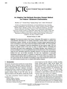
Figure 1. For each triangle T ∈ Tℓ , there is one fixed reference edge, indicated by the double line (left, top). Refinement of T is done by bisecting the reference edge, where its midpoint becomes a new node. The reference edges of the son triangles T ′ ∈ Tℓ+1 are opposite to this newest vertex (left, bottom). To avoid hanging nodes, one proceeds as follows: We assume that certain edges of T , but at least the reference edge, are marked for refinement (top). Using iterated newest vertex bisection, the element is then split into 2, 3, or 4 son triangles (bottom). If all elements are refined by three bisections (right, bottom), we obtain the so-called uniform bisec(3)-refinement which is denoted by Tbℓ .

2.2. Meshes and local mesh-refinement. A triangulation T of Γ consists of compact S 2-dimensional simplices (i.e., triangles) T such that T ∈T T = Γ. We do not allow hanging nodes. The volume area |T | of every element defines the local mesh-width hT ∈ L∞ (Γ) by hT |T := hT (T ) := |T |1/2 . We define ET to be the set of all edges e of the triangulation T , and NT as the set of all nodes z of the triangulation which are not on the boundary ∂Γ. We will need different kinds of patches. For a node z ∈ NT , we denote by ωz the node patch as the set of all elements T ∈ T sharing z. Likewise, we define an edge patch ωe . For an element T ∈ T , the patch ωT is the set of all elements sharing a node with T . Starting from an initial triangulation T0 of Γ, we will generate a sequence of meshes Tℓ for ℓ ∈ N via so-called newest vertex bisection (NVB). For a brief overview, we refer to Figure 1, and for a precise definition, we refer the reader to [Ver96, KPP13]. We denote by T a fixed reference element, and by u the pull-back of a function u defined on T , i.e., if FT : T → T is the affine element map, u := u ◦ FT . An important property of the NVB refinement strategy is that one can not only map elements T to fixed reference domains, but also patches. This means that there is a finite set of fixed reference patches and affine maps such that any node-, element-, or edge patch is the affine image of such a reference patch. In particular, there are only finitely many constants involved in scaling argument on patches, and hence, one may use patches in scaling arguments. For a mesh T , we denote by Tb the uniformly refined mesh, i.e., all edges in T are bisected. For a triangle T ∈ T , we denote by nT the normal vector on ∂T pointing outwards of T . For an inner edge e ∈ ET , i.e., e ⊂ Γ, we denote by Te+ and Te− the two elements of T sharing e, and we define n+ := nTe+ and n− := nTe− . For smooth enough functions φ : Γ → R and v : Γ → R2 we define the jumps J·K and averages {·} of the traces φ+ , φ− , v+ , and v− by {φ}|e := 21 (φ+ + φ− ), {v}|e := 21 (v+ + v− ), + + − − JφK|e := φ n + φ n , JvK|e := v+ n+ + v− n− . If we equip a mesh with an index, e.g., Tℓ , then we will use the index (·)ℓ instead of (·)Tℓ , i.e., we write, e.g., hℓ instead of hTℓ , and the same abbreviation will be used for sets of edges or nodes, e.g., Eℓ or Nℓ .

6


2.3. Crouzeix-Raviart boundary elements. For a given mesh T , P 1 (T ) is the space of piecewise linear functions. By V 0 = VT0 , we denote the space of lowest-order continuous boundary elements, i.e., V 0 := P 1 (T ) ∩ H01 (Γ), and V = VT is the space of Crouzeix-Raviart boundary elements, i.e., ( ) Φ is continuous in m ∀e ∈ E with e * ∂Γ, e T V := Φ ∈ P 1 (T ) , Φ(me ) = 0 ∀e ∈ ET with e ⊂ Γ where me is the midpoint of e ∈ ET . For curlT : P 1 (T ) → L2 (Γ) being the T -piecewise tangential curl operator, a norm in V is given by ||| · |||T := kcurlT · kH e −1/2 (Γ) . In the following we consider the bilinear form aT (Φ, Ψ) := hVcurlT Φ , curlT Ψi. By the properties of the single-layer operator V, cf. [McL00], aT is symmetric and there is a constant Cnorm > 1, independent of T and Φ ∈ V , such that −2 2 Cnorm |||Φ|||2T ≤ aT (Φ, Φ) ≤ Cnorm |||Φ|||2T .

This makes aT an inner product in V , which is therefore a Hilbert space. Assuming additional regularity f ∈ H −1/2+ε (Γ) with ε > 0, then (6)

hf , Ψi ≤ kf kH −1/2+ε (Γ) kΨkH 1/2−ε (Γ) ≤ CT |||Ψ|||T

for all Ψ ∈ V.

Here we used the equivalence of norms in the finite-dimensional space V , such that the number CT > 0 depends on T . By the Lax-Milgram lemma there exists a unique Galerkin solution Φ ∈ V of (7)

hVcurlT Φ , curlT Ψi = hf , Ψi

for all Ψ ∈ V.

The unique solvability of (7) was already addressed in [HS09] and studied via an equivalent saddle-point problem. We emphasize that the constant CT in (6) depends on V , but is not used in our analysis. In the statements and arguments below, our notations will mostly omit the explicit dependence on T by writing, e.g., ||| · |||, assuming that this is the norm related to the finest mesh which occurs in the norms’ argument. 2.4. Uniform refinement: consistency error and optimal convergence. We briefly discuss existing results for the Crouzeix-Raviart BEM of Section 2.3 based on a sequence of uniformly refined meshes (Tℓ )ℓ∈N0 . According to [HS09, Theorem 2], it holds that (8)

1/2

|||φ − Φℓ ||| . hℓ kφkH 1 (Γ) ,

if f ∈ L2 (Γ) and (Tℓ )ℓ∈N0 is a uniform sequence of meshes with mesh width hℓ . The proof of (8) uses, as is customary in the analysis of non-conforming methods, the Lemma of Berger, Scott, and Strang, see, e.g., [BSS72]. With a view to the well-known approximation results of conforming method, it suffices to bound the so-called consistency error. In [HS09, Prop. 5], it is shown that this can be done by #1/2 " X a(φ − Φℓ , Ψℓ ) 2 sup kte · Vcurlφ − µℓ kL2 (e) . inf0 µℓ ∈P (Eℓ ) Ψℓ ∈Vℓ kcurlΓ Ψℓ kH e −1/2 (Γ) e∈E ℓ

ADAPTIVE CR-BEM

7

1

0.1

0.01

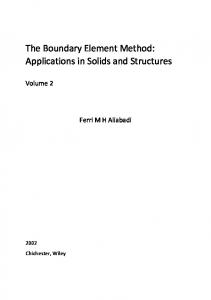
µ e2ℓ ηℓ2 ρ2ℓ + ρb2ℓ |||Φℓ − Φ0ℓ |||2 N −1/2 10

100

1000

Degrees of freedom Figure 2. Convergence rates for uniform mesh refinement and smooth solu−1/2 tion. Note that we plot squared quantities, so that O(Nℓ ) corresponds to 1/2 rate of O(hℓ ) for the original quantities. 1/2

and that the right-hand side converges like O(hℓ ), see [HS09, Lemma 6]. However, this bound for the convergence rate of the right-hand side is optimal. Indeed, for v ∈ P 1 (Γ)\P 0 (Γ) it holds that #1/2 " X 1/2 kv − µℓ k2L2 (e) ≃ O(hℓ ), inf0 µℓ ∈P (Eℓ )

e∈Eℓ

which can be seen by a direct calculation. Therefore, we are led to conjecture that the optimal order of convergence is O(h1/2 ). An easy numerical example supports this conjecture. We choose Γ = [0, 1]2 and divide it along the diagonals and the midpoints of its sides, such that we obtain a mesh T0 of 8 triangles. We choose the exact solution φ ∈ V00 that vanishes on ∂Γ and has the value 1 in the center of Γ. In Figure 2, we visualize the outcome of the corresponding Crouzeix-Raviart BEM based on a uniform mesh refinement. We have not yet defined the shown quantities, but what is important here is that Φℓ ∈ Vℓ denotes the Crouzeix-Raviart solution on the mesh Tℓ , whereas Φ0ℓ ∈ Vℓ0 denotes the conforming solution. According to the definition of φ, we have Φ0ℓ = φ, and hence, according to (8), 1/2

|||Φℓ − Φ0ℓ ||| = |||φ − Φℓ ||| = O(hℓ ). e 1/2 (Γ) ∩ H 3/2−ε (Γ). One would expect an increased order of O(h1−ε ℓ ) for every ε > 0, as φ ∈ H 1/2 However, as Figure 2 reveals, this increased rate is not achieved - we still observe O(hℓ ), which therefore seems to be the optimal rate that can be obtained. 3. Preliminaries

8


3.1. Conforming approximations and partial orthogonality. For the development and analysis of the adaptive Crouzeix-Raviart boundary elements, it will be convenient to use a decomposition of the space VT into conforming and non-conforming components. Such a decomposition is given by the identity VT = VT0 ⊕ VT⊥ , where VT⊥ is the orthogonal complement of VT0 with respect to the inner product aT (·, ·). For a function Φ ∈ VT , we write Φ = Φ0 + Φ⊥ with Φ0 ∈ VT0 and Φ⊥ ∈ VT⊥ . We emphasize that there is a partial orthogonality, i.e., if T⋆ is a refinement of T , then a⋆ (φ − Φ⋆ , Ψ) = 0

for all Ψ ∈ VT0 ,

where φ is the exact solution and Φ⋆ ∈ VT⋆ is its non-conforming Galerkin approximation. In contrast to conforming methods, this orthogonality property cannot be extended to all Ψ ∈ VT . However, it can be extended to a partial orthogonality as follows, cf. [BN10, Corollary 4.3]. Lemma 1. Let T⋆ be a refinement of T and Φ⋆ ∈ VT⋆ the Galerkin solution (7) on T⋆ . Then, for all ε > 0, and all Φ ∈ VT , we have a⋆ (φ − Φ⋆ , φ − Φ⋆ ) ≤ (1 + ε)a(φ − Φ, φ − Φ) −2 Cnorm 1 2 2 −2 − |||Φ − Φ⋆ |||⋆ + Cnorm (1 + ) + Cnorm |||(Φ − Φ0 ) − (Φ⋆ − Φ0⋆ )|||2⋆ 2 ε

Proof. As φ − Φ⋆ is orthogonal to VT0 and V 0 (T⋆ ), we have

a⋆ (φ − Φ⋆ , φ − Φ⋆ ) = a⋆ (φ − Φ⋆ − Φ0 + Φ0⋆ , φ − Φ⋆ − Φ0 + Φ0⋆ ) − a⋆ (Φ0⋆ − Φ0 , Φ0⋆ − Φ0 ) ⊥ ⊥ 0 0 0 0 = a⋆ (φ − Φ + Φ⊥ − Φ⊥ ⋆ , φ − Φ + Φ − Φ⋆ ) − a⋆ (Φ⋆ − Φ , Φ⋆ − Φ )

= a⋆ (φ − Φ, φ − Φ) + 2a⋆ (Φ⊥ − Φ⊥ ⋆ , φ − Φ) 0 0 0 0 ⊥ ⊥ + a⋆ (Φ⊥ − Φ⊥ ⋆ , Φ − Φ⋆ ) − a⋆ (Φ⋆ − Φ , Φ⋆ − Φ ),

where we used the identity Φ⋆ + Φ0 − Φ0⋆ = Φ − Φ⊥ + Φ⊥ ⋆ in the second step. Using the stability, ellipticity, and Young’s inequality ab ≤ a2 /(4ε) + εb2 , we obtain 1/2 ⊥ ⊥ 1/2 2a⋆ (φ − Φ, Φ⊥ − Φ⊥ a⋆ (Φ⊥ − Φ⊥ ⋆ ) ≤ 2a(φ − Φ, φ − Φ) ⋆ , Φ − Φ⋆ ) 2 2 ≤ εa(φ − Φ, φ − Φ) + ε−1 Cnorm |||Φ⊥ − Φ⊥ ⋆ |||⋆ ,

as well as −2 Cnorm −2 ⊥ 2 −2 0 0 2 0 0 0 0 |||Φ⋆ − Φ|||2⋆ − Cnorm |||Φ⊥ ⋆ − Φ |||⋆ ≤ Cnorm |||Φ⋆ − Φ |||⋆ ≤ a⋆ (Φ⋆ − Φ , Φ⋆ − Φ ). 2

Finally, the estimate ⊥ ⊥ 2 ⊥ ⊥ 2 a⋆ (Φ⊥ − Φ⊥ ⋆ , Φ − Φ⋆ ) ≤ Cnorm |||Φ − Φ⋆ |||⋆

concludes the proof.

ADAPTIVE CR-BEM

9

e −1/2 (Γ). Lemma 1 will be the basis for the anal3.2. Quasi-interpolation operators in H ysis of the a posteriori error estimators in Section 4, such that terms of the form |||Φ − Φ0 ||| will emerge. Those terms are (in principle) computable. However, they involve conforming approximations Φ0 , which we don’t want to compute, and hence we need to find a substitute involving only Φ. This will be done in Corollary 6, where we will estimate the nonconformity of a function Φ by its jumps over edges. The proof of this corollary will be based on results of the present section, the aim of which is to provide an interpolation operator to approximate the conforming part Φ0 of a given function Φ. We will use the well-known interpolation opere −1/2 (Γ). ator IT by Clément [Clé75, SZ90], and provide approximation results in the space H For a function v ∈ L2 (Γ), this operator is defined as X (9) ψ(z)ϕz , IT v := z∈NT

where ϕz is the nodal basis function of VT0 associated with the node z ∈ NT . The function ψ ∈ VT0 |ωz is such that Z (v − ψ)ϕ = 0 for all ϕ ∈ VT0 |ωz ωz

see also [BN10, Lemma 6.6]. In addition, we denote by ΠT the L2 (Γ) orthogonal projection onto the space of piecewise constants [P 0 (T )]2 . The well-known properties of the operator IT are collected in the following lemma. We again refer to [BN10, Lemma 6.6] for a proof. Lemma 2. Let T be a refinement of T0 . Then, there exists a constant CI which depends only on T0 such that (10)

kIT ϕkL2 (Γ) ≤ CI kϕkL2 (Γ)

and

kIT ϕkH 1 (Γ) ≤ CI kϕkH 1 (Γ) ,

and such that for all T ∈ T , for all ϕ ∈ H01 (Γ), and for all Φ ∈ VT , it holds that (11a)

kϕ − IT ϕkL2 (T ) ≤ CI khT ∇ϕkL2 (ωT ) ,

(11b)

kΦ − IT ΦkL2 (T ) ≤ CI khT JΦKkL2 (EωT ) ,

1/2

−1/2

k∇T (Φ − IT Φ)kL2 (T ) ≤ CI khT

(11c)

JΦKkL2 (EωT ) .

e −1/2 (Γ). To do For our purposes, we need to analyze the properties of IT in the space H so, we will use integration by parts piecewise. The resulting integrals over the skeleton ET will be bounded with the aid of the following auxiliary result. Lemma 3. Let T be a refinement of T0 with the set of edges ET . Then, there is a constant 2 Cedge which depends only on T0 such that for any choice of functions Φ ∈ VT and V ∈ [VT0 ] , it holds that Z (12) JΦK{V} ≤ Cedge kJΦKkL2 (ET ) kVkH1/2 (Γ) . ET

b ∈ V 0 , it holds that Furthermore, if Tb is the uniform refinement of T and Φ Tb Z 1/2 b b L2 (Γ) kVkH1/2 (Γ) . JΦK{V} ≤ Cedge khT (1 − ΠT )∇Tb Φk (13) ETb

10


Proof. For every edge e ∈ ET , we use an affine map to transfer the edge patch ωe to a reference configuration ωe . As we emphasized in Section 2.2, the number of this reference configurations is bounded uniformly, which permits us to use scaling arguments. Now we choose ce ∈ R2 such that kV − ce kL2 (e) . |V|H1/2 (ωe ) , slo

which is possible since V is an element of a finite dimensional space. Here, the index slo indicates that the norm is defined according to Sobolev-Slobodeckij. Mapping both sides back to the physical domain yields kV − ce kL2 (e) . |V|H1/2 (ωe ) ≤ kVkH1/2 (ωe ) .

(14)

slo

slo

As Φ is a Crouzeix-Raviart function, its jump JΦK has vanishing integral mean on every edge e ∈ ET , and hence, using the Cauchy-Schwarz inequality, we obtain with (14) !1/2 !1/2 Z X X XZ kV − ce k2L2 (e) kJΦKk2L2 (e) JΦK{V − ce } ≤ JΦK{V} = ET

e∈ET

e

e∈ET

≤

X

kJΦKk2L2 (e)

e∈ET

!1/2

e∈ET

X

kVk2H1/2 (ω slo

e∈ET

e)

!1/2

.

1/2

Locally, only three patches ωe overlap, and the fact that the norms Hslo (Γ) and H1/2 (Γ) are equivalent finally concludes the proof of (12). Now we prove (13). We start at (12), this time with Tb instead of T , to obtain 1/2  Z X b 2L (e)  kVkH1/2 (Γ) . b kJΦKk JΦK{V} . 2 ETb

e∈ETb

b over the skeleton E b into the contributions on the Now we split the L2 norm of the jump JΦK T skeleton ET and the rest, which we write sloppy as ETb \ ET . Then, X X X b 2 b 2 . b 2 kJ ΦKk + (15) kJΦKk kJΦKk = L2 (e) L2 (e) L2 (e) e∈ETb

e∈ET

e∈ETb \ET

b such that We claim that there is a constant C > 0, independent of ETb and Φ b L2 (ωe ) b L2 (e) ≤ Ch1/2 k(1 − ΠT )∇ b Φk kJΦKk e T b L (e) ≤ Ch1/2 k(1 − ΠT )∇ b Φk b L (T ) kJΦKk 2 e 2 T

if e ∈ ET ,

if e ∈ ETb \ ET with e ⊂ T ∈ T .

Both sides define seminorms, and the left one vanishes when the right one does. Hence, the bounded dimension of the underlying space and a scaling argument prove the claim. Using the last two estimates in (15) shows (13). Lemma 4. In addition to Lemma 2, we have the following estimates, where Tb denotes the b ∈ V b , it holds that uniform refinement of T : For Φ ∈ VT and Φ T (16a)

′ k∇T (1 − IT )ΦkH e −1/2 (Γ) ≤ CI khT JΦK kL2 (ET ) ,

(16b)

b e −1/2 ≤ CI kh (1 − ΠT )∇ b Φk b L (Γ) . k∇Tb (1 − IT )Φk 2 T H (Γ) T

1/2

ADAPTIVE CR-BEM

11

Proof. We will use estimates (10) and (11) to prove this lemma. First, if we denote by IT v the component-wise action of IT to v ∈ H1/2 (Γ), we integrate by parts piecewise to obtain XZ h∇T (1 − IT )Φ , IT vi = −h(1 − IT )Φ , divIT vi + (Φ − IT Φ)IT v · nT . T ∈T

ET

As JIT ΦK vanishes due to the continuity of IT Φ, the second term on the right-hand side can be written as Z Z XZ (Φ − IT Φ)IT v · nT = JΦ − IT ΦK{IT v} + {Φ − IT Φ}JIT vK T ∈T

ET

=

Z

ET

ET \∂Γ

JΦK{IT v}. ET

We conclude that, for any v ∈ H1/2 (Γ), h∇T (1 − IT )Φ , vi = h∇T (1 − IT )Φ , v − IT vi − h(1 − IT )Φ , divIT vi Z (17) + JΦK{IT v}. ET

We bound the terms on the right-hand side separately. Taking into account (11c), the first term on the right-hand side of (17) can be estimated by X h∇T (1 − IT )Φ , v − IT vi ≤ k∇T (1 − IT )ΦkL2 (T ) kv − IT vkL2 (T ) T ∈T

(18)

.

X

−1/2

hT |T

kJΦKkL2 (EωT ) kv − IT vkL2 (T )

T ∈T

−1/2

≤ kJΦKkL2 (ET ) khT −1/2

Now, it holds that khT the estimates

(v − IT v)kL2 (Γ) .

(v − IT v)kL2 (Γ) . kvkH1/2 (Γ) , which follows from interpolation of

kv − IT vkL2 (Γ) . kvkL2(Γ)

and

kh−1 T (v − IT v)kL2 (Γ) . kvkH1 (Γ) ,

which themselves can be derived summing (10) and (11a) over the elements of the mesh. We conclude that (19)

h∇T (1 − IT )Φ , v − IT vi . kJΦKkL2 (ET ) kvkH1/2 (Γ) .

The second contribution on the right-hand side of (17) can be bounded by using (11b) via X hΦ − IT Φ , divIT vi ≤ kΦ − IT ΦkL2 (T ) kdivIT vkL2 (T ) T ∈T

(20)

1/2

. kJΦKkL2 (ET ) khT divIT vkL2 (Γ) . kJΦKkL2 (ET ) kvkH1/2 (Γ) .

In the last step we used an inverse estimate, cf. [CP07, Proposition 3.1] and the recent extension [AFF+ 13b, Proposition 5], and the fact that IT is bounded in H1/2 (Γ), which again follows by interpolation, this time using the estimates (10). The third part on the right-hand side of (17) can be bounded by Lemma 3 and the H1/2 (Γ)-boundedness of IT via Z (21) JΦK{IT v} . kJΦKkL2 (ET ) kvkH1/2 (Γ) . ET

12


From the identity (17) we conclude, using (19), (20), and (21), that k∇T (1 − IT )ΦkH e −1/2 (Γ) =

sup

h∇T (1 − IT )Φ , vi . kJΦKkL2 (ET ) .

kvkH1/2 (Γ) =1

From this, (16a) follows from a Poincaré inequality, which may be used since Φ ∈ VT implies that the jump JΦK vanishes at the midpoint of every element. To prove (16b), we again use integration by parts piecewise and conclude as before (22)

b , vi = h∇ b (1 − IT )Φ b , v − IT vi − h(1 − IT )Φ b , divIT vi, h∇Tb (1 − IT )Φ T Z b T v}. + JΦK{I ETb

The first and second term can be bounded as in (18) and (20), this time using the local estimates b L (T ) ≤ Ck(1 − ΠT )∇ b Φk b L (ω ) k∇ b (1 − IT )Φk T

2

T

2

T

b L (T ) ≤ ChT |T k(1 − ΠT )∇ b Φk b L (ω ) , k(1 − IT )Φk 2 2 T T

which follow from a scaling argument and norm equivalence in finite dimensional spaces. The last term in (22) can be bounded by (13) of Lemma 3. We will also need the following boundedness result for IT . Lemma 5. In addition to Lemma 2, we have the following estimate, where Tb denotes the b ∈ V b , it holds that uniform refinement of T : For Φ ∈ VT and Φ T (23)

b e −1/2 ≤ CI k∇ b Φk b e −1/2 . k∇T IT Φk H (Γ) T H (Γ)

Proof. To prove (23), we first observe that due to the local L2 boundedness of (1 − ΠT ) and the inverse estimate [GHS05, Thm. 3.6], we have 1/2 b L2 (Γ) ≤ kh1/2 ∇ b Φk b e −1/2 . b L2 (Γ) . k∇ b Φk khT (1 − ΠT )∇Tb Φk T H (Γ) T T

Hence, the triangle inequality and (16b) show

b e −1/2 . b e −1/2 . k∇ b Φk b e −1/2 + k∇ b (1 − IT )Φk b e −1/2 ≤ k∇ b Φk k∇Tb IT Φk H (Γ) T H (Γ) T H (Γ) H (Γ) T

4. A posteriori error estimation and adaptive algorithm In this section, we introduce different error estimators, and show their reliability and efficiency. In Section 4.1, we introduce global error estimators, that is, the employed (noninteger) norm is nonlocal and therefore does not provide information for local mesh-refinement. In Section 4.2, we pass over to weighted (integer) norms, which are local and can therefore be employed in an adaptive algorithm, which will be introduced in Section 4.3. In order to estimate the nonconformity of a function in terms of the function itself, we will use the results of Sections 3.1 and 3.2. Corollary 6. Denote by T a refinement of T0 . Let Φ ∈ VT be the Galerkin solution (7). Then, there is a constant C4 > 0 which depends only on T0 such that |||Φ⊥ |||T = |||Φ − Φ0 |||T ≤ C4 khT JΦK′ kL2 (ET ) .

ADAPTIVE CR-BEM

13

Proof. This follows easily by using the fact that Φ − Φ0 is aT -orthogonal to VT0 and employing (16a). b ∈ V b be Galerkin solutions (7), where 4.1. Global error estimators. Let Φ ∈ VT and Φ T Tb is a uniform refinement of T . We introduce estimators on the mesh T by b − Φ||| b = kcurl b (Φ b − Φ)k e −1/2 , ηT := |||Φ T T H (Γ)

b − IT Φ||| b b = kcurl b (Φ b − IT Φ)k b e −1/2 . ηeT := |||Φ T T H (Γ)

The existing derivations of h − h/2 error estimators, e.g. [EFLFP09, FLP08], focus on conforming methods and rely mostly on the Galerkin orthogonality (3). Contrary, we have the weaker partial orthogonality of Lemma 1, where additional terms arise (what we called nonconformity error) which account for the nonconformity. In Corollary 6, we showed that these terms can be bounded by the inter-element jumps of Φ, i.e., by ρT := khT JΦK′ kL2 (ET ) . Consequently, we have that ηT and ηeT are equivalent up to ρT .

Lemma 7. Let T be a refinement of T0 . Then, there is a constant C5 > 0 which depends only on T0 such that b − IT Φ||| b b + ρT b − Φ||| b ≤ |||Φ C5−1 |||Φ T T

and

b − Φ||| b + ρT . b − IT Φ||| b b ≤ |||Φ C5−1 |||Φ T T

b − Φ is orthogonal to V 0 in a b , we conclude Proof. As Φ T T

b − Φ + Φ0 − IT Φ||| b ≤ |||Φ b − IT Φ||| b b + |||Φ − Φ0 |||T , b − Φ||| b . |||Φ |||Φ T T

and the last term can be bounded by ρT by Corollary 6. To see the second estimate, we use the projection property and boundedness (23) of IT to see that b − IT Φ||| b b . |||Φ b − Φ0 ||| b ≤ |||Φ b − Φ||| b + |||Φ − Φ0 |||T , |||Φ T T T

which shows the desired estimate.

In a next step, we show the efficiency and reliability of ηT . For the reliability, we assume that a saturation assumption for the conforming approximations holds true. Theorem 8. Let T be a refinement of T0 . Then, there is a constant Ceff > 0 such that b − Φ||| b is efficient up to the nonconformity error, i.e., ηT = |||Φ T (24)

−1 b Ceff |||Φ − Φ|||Tb ≤ |||φ − Φ|||T + ρT + ρTb .

Furthermore, assume that there is a constant Csat ∈ (0, 1) such that the saturation assumption for the conforming approximations (25)

b 0, φ − Φ b 0 ) ≤ Csat aT (φ − Φ0 , φ − Φ0 ) aTb (φ − Φ

b − Φ||| b is reliable up to holds true. Then, there is a constant Crel > 0 such that ηT = |||Φ T ρT + ρTb , i.e., (26)

holds true.

−1 b − Φ||| b + ρT + ρ b Crel |||φ − Φ|||T ≤ |||Φ T T

14


Proof. Efficiency (24) follows immediately from Lemma 1 by setting T⋆ := Tb and Corollary 6. To show reliability (26), we first note that the triangle inequality and ellipticity give |||φ − Φ||| . a(φ − Φ0 , φ − Φ0 ) + ρT .

Now, due to the conforming orthogonality and the saturation assumption (25), b 0 , Φ0 − Φ b 0 ) . |||Φ0 − Φ b 0 ||| b (1 − Csat )a(φ − Φ0 , φ − Φ0 ) ≤ a(Φ0 − Φ T 0 b − Φ||| b + |||Φ − Φ ||| + |||Φ b −Φ b 0 ||| ≤ |||Φ T

b − Φ||| b + ρT + ρ b , . |||Φ T T

where we used the triangle inequality and Corollary 6.

Remark 9. In finite element methods, the saturation assumption (25) is verified for the Poisson problem −∆u = f . In fact, in [DN02] it is shown that b 0ℓ ||| ≤ Csat |||φ − Φ0ℓ ||| + oscℓ , |||φ − Φ

where oscℓ is a measure for the resolution of f on the mesh Tℓ . Hence, small data oscillation implies the saturation assumption. However, the saturation assumption (25) is not proven for BEM. To the best of the our knowledge, the only contributions are [AFF+ 13a, EH06]. In [AFF+ 13a], it is shown that for 2D-BEM for the weakly singular integral equation, there is a k ∈ N and Csat < 1 which depend only on T0 and Γ, such that with k uniform refinements of Tℓ , which we denote by Tℓ(k) , there holds |||φ − Φℓ ||| ≤ Csat |||φ − Φℓ(k) ||| + oscℓ with oscℓ being a term of higher order than the others. In [EH06], the saturation assumption is analyzed for an edge singularity on a plane square-shaped domain, and uniform as well as graded meshes are considered. e −1/2 (Γ)4.2. Localized error estimators. The a posteriori estimators of Section 4.1 use the H norm, which is hard to compute and nonlocal. In order to provide a posteriori error estimators which can be split into element-wise indicators, we will use a weighted L2 -norm. We introduce the localized estimators 1/2 b − Φ)kL2 (Γ) , µT := kh curl b (Φ µ eT :=

T T 1/2 b khT (curlTb Φ

Then we have the following result.

Lemma 10. There holds 1/2 b − ΠT curl b Φ)k b L kh (curl b Φ (27a) T

T

T

1/2

2 (Γ)

and

(27b)

b L2 (Γ) . − ΠT curlTb Φ)k

1/2

b − Φ)kL (Γ) . |||Φ b − Φ||| b ≤ khT curlTb (Φ 2 T

b − IT Φ||| b b . kh (curl b Φ b − ΠT curl b Φ)k b L2 (Γ) . |||Φ T T T T

In particular, all estimators are equivalent up to ρT + ρTb , and for τ ∈ {ηT , ηeT , µT , µ eT }, the estimator τ is reliable and efficient up to ρT + ρTb , i.e., |||φ − Φ||| . τ + ρT + ρTb ,

τ . |||φ − Φ||| + ρT + ρTb .

ADAPTIVE CR-BEM

15

Proof. As in [FLP08], the first estimate in (27a) follows from the best approximation property of ΠT , while the second one follows from the inverse inequality [GHS05, Theorem 3.6]. The first estimate in (27b) is estimate (16b) from Lemma 4. Now, since b − Φ||| b ηT = |||Φ T

b − IT Φ||| b b ηeT = |||Φ T

and

are equivalent up to ρT + ρTb according to Lemma 7, all estimators are equivalent up to ρT + ρTb as well. As ηT is efficient and reliable up to ρT + ρTb according to Theorem 8, this is also true for the three other estimators. 4.3. Statement of the adaptive algorithm. We now introduce the adaptive algorithm. As error indicators on a mesh Tℓ , we use the element-wise quantities 1/2 b b 2 b ℓ k2L (T ) + khℓ JΦℓ Kk2 1 ̺ℓ (T )2 := khℓ (1 − Πℓ )curlTbℓ Φ H (Eℓ (T )) + khℓ JΦℓ KkH 1 (Eb (T )) . 2 ℓ

For a subset Mℓ ⊂ Tℓ , we write ̺ℓ (Mℓ )2 = ̺ℓ := ̺ℓ (Tℓ ). Hence,

P

T ∈Mℓ

̺ℓ (T )2 , and we use the abbreviation

̺2ℓ = µ e2ℓ + ρ2ℓ + ρb2ℓ

is a reliable error estimator according to Lemma 10. The adaptive algorithm now reads as follows. Algorithm 11. Input: Initial mesh T0 , parameter θ ∈ (0, 1), counter ℓ := 0. (i) (ii) (iii) (iv) (28)

Obtain Tbℓ by uniform bisec(3)-refinement of Tℓ , see Figure 1. b ℓ of (7) with respect to Tℓ and Tbℓ . Compute solutions Φℓ and Φ Compute refinement indicators ̺ℓ (T ) for all T ∈ Tℓ . Choose a set Mℓ ⊆ Tℓ with minimal cardinality such that X X ̺ℓ (T )2 . ̺ℓ (T )2 ≥ θ T ∈Mℓ

T ∈Tℓ

(v) Refine mesh Tℓ according to Algorithm NVB and obtain Tℓ+1 . (vi) Update counter ℓ := ℓ + 1 and goto (i). 5. Numerical experiments In this section we present numerical experiments for two different problems. The exact solution φ of the first experiment will be smooth in the sense that uniform and adaptive mesh refinement yield the same rate of convergence. Still, φ exhibits singularities which stem from the geometric setting (i.e., polygonal boundary). As we emphasized in the introduction, it is a peculiarity of Crouzeix-Raviart BEM that uniform mesh refinement is optimal for these kind of singularities. The second example reports on a case where the right-hand side of our model problem is chosen to be singular, such that, due to the mapping properties of W, the exact solution φ suffers from low regularity as well. In this case, it will turn out that uniform mesh-refinement is suboptimal while adaptive refinement recovers the optimal rate.

16


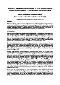
Figure 3. Initial mesh T0 used in the numerical experiments. 5.1. Experiment with smooth solution. We consider the screen Γ := [0, 1]2 . The initial mesh T0 consists of 8 congruent triangles, cf. Fig. 3, such that Γ is halved along the diagonals and the midpoints of its sides. The reference edges are chosen on the two diagonals. The right-hand side is given by f (x, y) = 1, and it is well known that the exact solution φ has square root edge singularities [Ste87] so e 1−ε (Γ) for all ε > 0. We use the following five different sequences of meshes. that φ ∈ H Uniform sequence, Figure 4. The sequence Tℓ , ℓ ∈ N0 , is generated by uniform refinement, i.e., the initial mesh T0 is chosen as in Figure 3, and the mesh Tℓ , ℓ ≥ 1 is generated from Tℓ−1 by a bisec(3)-refinement (as described in Figure 1) of every triangle T ∈ Tℓ . Due to 1/2−ε −1/4+ε the results in [HS09], we expect a convergence rate of O(hℓ ) = O(Nℓ ) for all ε > 0, cf. (8). This is exactly what we observe in the convergence history in Fig. 4. Adaptive sequence, Figure 5. The sequence of meshes Tℓ , ℓ ∈ N0 , is generated by Algorithm 11 with θ = 0.5, where T0 is chosen as in Figure 3. As we conjectured in Section 2.4, −1/4 the rate O(Nℓ ) cannot be improved in general, and this is what we see in the convergence history in Fig. 5. In Fig. 8 we plot the intermediate mesh T11 and the final mesh T22 that are constructed by the adaptive algorithm. What we observe qualitatively is that the meshes are refined towards the boundary ∂Γ, which meets the expectation as φ exhibits singularities there. Nevertheless, the computed meshes are not optimal for a conforming method. This is visualized in Fig. 5, where we also plot the conforming energy error |||φ − Φ0ℓ |||2. Clearly, we use the number of the degrees of freedom of the conforming method for the x-axis. Graded sequence, Figs. 6 and 7. We use a sequence of meshes Tℓ , ℓ ∈ N0 that is graded towards ∂Γ, i.e., for all elements T ∈ Tℓ there holds hℓ (T ) ≃ dist(T, Γ)β . We select the parameters β ∈ {2, 3}. The numerical results show that both gradings maintain the optimal rate for the Crouzeix-Raviart BEM, see Figs. 6 and 7. 5.2. Experiment with singular solution. The right-hand side is given by f (x, y) := x−6/10 ,

ADAPTIVE CR-BEM

17

10

1

0.1

0.01

0.001

µ e2ℓ

ρ2ℓ + ρb2ℓ

ηℓ2

|||Φℓ − Φ0ℓ |||2

10

100

−1/2

Nℓ

1000

10000

Degrees of freedom Figure 4. Convergence history for uniform mesh refinement and smooth so−1/2 lution. We see that the squared quantities exhibit the optimal rate O(Nℓ ). 10

1

0.1

0.01

0.001

1

µ e2ℓ

ρ2ℓ + ρb2ℓ

ηℓ2

|||Φℓ − Φ0ℓ |||2 10

100

|||φ − Φ0ℓ |||2 −1/2

Nℓ 1000

10000

Degrees of freedom Figure 5. Convergence history for adaptive algorithm and smooth solution. −1/2 We see that the squared quantities exhibit the optimal rate O(Nℓ ). and because of f ∈ / L2 (Γ) we conclude from the mapping properties of W that the exact solution fulfills φ ∈ / H 1 (Γ). The missing regularity will lead to a suboptimal convergence rate for uniform refinement, which will be recovered by the adaptive algorithm. Let us

18


10

1

µ e2ℓ

ρ2ℓ + ρb2ℓ

ηℓ2

|||Φℓ − Φ0ℓ |||2

−1/2

Nℓ

0.1

0.01

1000

10000

Degrees of freedom Figure 6. Convergence history for graded meshes with β = 2 and smooth −1/2 solution. We see that the squared quantities exhibit the optimal rate O(Nℓ ). 1000

100

10

µ e2ℓ

ρ2ℓ + ρb2ℓ

ηℓ2

|||Φℓ − Φ0ℓ |||2

−1/2

Nℓ

1

0.1

0.01

1000

10000

Degrees of freedom Figure 7. Convergence history for graded meshes with β = 3 and smooth −1/2 solution. We see that the squared quantities exhibit the optimal rate O(Nℓ ). briefly discuss what to expect in the uniform case: for the function g(x) = xα there holds g ∈ H α+1/2−ε (0, 1) \ H α+1/2 (0, 1) for all ε > 0. We conclude that, f ∈ H −0.1−ε (Γ) \ H −0.1 (Γ),

ADAPTIVE CR-BEM

19

Figure 8. Meshes T11 and T22 of the adaptive algorithm for smooth solution. e 9/10 (Γ). Hence, we expect and due to the mapping properties of W we conclude that φ ∈ /H 4/10 −1/5 a convergence rate which is worse than O(hℓ ) = O(Nℓ ) for uniform refinement. We already stated the choice of the initial mesh T0 . Uniform and adaptive meshes are computed exactly as described in Section 5.1. The convergence history for the uniform sequence of meshes is depicted in Fig. 9. We see that the uniform scheme is suboptimal, and the the −1/5 convergence rate is indeed worse than O(Nℓ ) (note that we plot squared quantities). However, the adaptive sequence of meshes, depicted in Fig. 10, recovers the optimal convergence rate. In Fig. 11, we plot the two adaptive meshes T11 and T23 which are generated by the adaptive algorithm. References [AFF+ 13a] Markus Aurada, Michael Feischl, Thomas Führer, Michael Karkulik, and Dirk Praetorius. Efficiency and Optimality of Some Weighted-Residual Error Estimator for Adaptive 2D Boundary Element Methods. Comput. Methods Appl. Math., 13(3):305–332, 2013. [AFF+ 13b] Markus Aurada, Michael Feischl, Thomas Führer, Michael Karkulik, and Dirk Praetorius. Energy norm based error estimators for adaptive BEM for hypersingular integral equations. Asc report, Institute for Analysis and Scientific Computing, Vienna University of Technology, 2013. [AO00] Mark Ainsworth and J. Tinsley Oden. A posteriori error estimation in finite element analysis. Pure and Applied Mathematics (New York). Wiley-Interscience [John Wiley & Sons], New York, 2000. [Ban96] Randolph E. Bank. Hierarchical bases and the finite element method. In Acta numerica, 1996, volume 5 of Acta Numer., pages 1–43. Cambridge Univ. Press, Cambridge, 1996. [BCS02] A. Buffa, M. Costabel, and D. Sheen. On traces for H(curl, Ω) in Lipschitz domains. J. Math. Anal. Appl., 276(2):845–867, 2002. [BH08] Alexei Bespalov and Norbert Heuer. The hp-version of the boundary element method with quasiuniform meshes in three dimensions. ESAIM Math. Model. Numer. Anal., 42(5):821–849, 2008. [BN10] Andrea Bonito and Ricardo H. Nochetto. Quasi-optimal convergence rate of an adaptive discontinuous Galerkin method. SIAM J. Numer. Anal., 48(2):734–771, 2010. [BSS72] Alan Berger, Ridgway Scott, and Gilbert Strang. Approximate boundary conditions in the finite element method. In Symposia Mathematica, Vol. X (Convegno di Analisi Numerica, INDAM, Rome, 1972), pages 295–313. Academic Press, London, 1972. [Clé75] Ph. Clément. Approximation by finite element functions using local regularization. RAIRO Analyse Numérique, 9(R-2):77–84, 1975.

20


100

10

1

0.1

µ e2ℓ

ρ2ℓ + ρb2ℓ

Nℓ

ηℓ2

|||Φℓ − Φ0ℓ |||2

Nℓ

10

100

−1/2

−2/5

1000

10000

Degrees of freedom Figure 9. Convergence history for uniform mesh refinement and singular right-hand side. The squared quantities do not exhibit the optimal rate, which −1/2 would be O(Nℓ ). 100

10

1

0.1

0.01

10

µ e2ℓ

ρ2ℓ + ρb2ℓ

ηℓ2

|||Φℓ − Φ0ℓ |||2 100

−1/2

Nℓ

1000

10000

Degrees of freedom Figure 10. Convergence history for adaptive algorithm and singular right−1/2 hand side. The squared quantities exhibit the optimal rate O(Nℓ ). [CP07]

Carsten Carstensen and Dirk Praetorius. Averaging techniques for the a posteriori BEM error control for a hypersingular integral equation in two dimensions. SIAM J. Sci. Comput., 29(2):782– 810 (electronic), 2007.

ADAPTIVE CR-BEM

21

Figure 11. Meshes T11 and T23 of the adaptive algorithm for singular solution.

[DH13]

Catalina Domínguez and Norbert Heuer. A posteriori error analysis for a boundary element method with non-conforming domain decomposition. http://arXiv.org/abs/1307.7310, 2013. Numer. Methods Partial Differential Eq., to appear. [DN02] Willy Dörfler and Ricardo H. Nochetto. Small data oscillation implies the saturation assumption. Numer. Math., 91(1):1–12, 2002. [EFLFP09] Christoph Erath, Samuel Ferraz-Leite, Stefan Funken, and Dirk Praetorius. Energy norm based a posteriori error estimation for boundary element methods in two dimensions. Appl. Numer. Math., 59(11):2713–2734, 2009. [EH06] Vincent J. Ervin and Norbert Heuer. An adaptive boundary element method for the exterior Stokes problem in three dimensions. IMA J. Numer. Anal., 26(2):297–325, 2006. [FLP08] Samuel Ferraz-Leite and Dirk Praetorius. Simple a posteriori error estimators for the h-version of the boundary element method. Computing, 83(4):135–162, 2008. [GHH09] Gabriel N. Gatica, Martin Healey, and Norbert Heuer. The boundary element method with Lagrangian multipliers. Numer. Methods Partial Differential Equations, 25(6):1303–1319, 2009. [GHS05] I. G. Graham, W. Hackbusch, and S. A. Sauter. Finite elements on degenerate meshes: inversetype inequalities and applications. IMA J. Numer. Anal., 25(2):379–407, 2005. [HNW87] E. Hairer, S. P. Nørsett, and G. Wanner. Solving ordinary differential equations. I, volume 8 of Springer Series in Computational Mathematics. Springer-Verlag, Berlin, 1987. Nonstiff problems. [HS09] Norbert Heuer and Francisco-Javier Sayas. Crouzeix-Raviart boundary elements. Numer. Math., 112(3):381–401, 2009. [KPP13] Michael Karkulik, David Pavlicek, and Dirk Praetorius. On 2D Newest Vertex Bisection: Optimality of Mesh-Closure and H 1 -Stability of L2 -Projection. Constr. Approx., 38(2):213–234, 2013. [McL00] William McLean. Strongly elliptic systems and boundary integral equations. Cambridge University Press, Cambridge, 2000. [Néd82] Jean-Claude Nédélec. Integral equations with nonintegrable kernels. Integral Equations Operator Theory, 5:562–572, 1982. [Ste87] Ernst P. Stephan. Boundary integral equations for screen problems in R3 . Integral Equations Operator Theory, 10:257–263, 1987. [SZ90] L. Ridgway Scott and Shangyou Zhang. Finite element interpolation of nonsmooth functions satisfying boundary conditions. Math. Comp., 54(190):483–493, 1990. [Tri95] Hans Triebel. Interpolation theory, function spaces, differential operators. Johann Ambrosius Barth, Heidelberg, second edition, 1995. [Ver96] Rüdiger Verfürth. A Review of A Posteriori Error Estimation and Adaptive Mesh-Refinement Techniques. B.G. Teubner, Stuttgart, 1996.

22


Facultad de Matemáticas, Pontificia Universidad Católica de Chile, Avenida Vicuña Mackenna 4860, Santiago, Chile E-mail address: {nheuer, mkarkulik}@mat.puc.cl URL: http://www.mat.puc.cl/{∼nheuer, ∼mkarkulik}

10

muTilde 1 eta coarse jumps inside conforming error N^{-1/2} 10

100

1000 N

10000

10

muTilde 1 eta coarse jumps inside conforming error N^{-1/2} 10

100

1000 N

10000