Adaptive Disk Spindown via Optimal Rent-to-Buy in Probabilistic

Algorithmica (1999) 23: 31–56

Algorithmica ©

1999 Springer-Verlag New York Inc.

Adaptive Disk Spindown via Optimal Rent-to-Buy in Probabilistic Environments1 P. Krishnan,2 P. M. Long,3 and J. S. Vitter4 Abstract. In the single rent-to-buy decision problem, without a priori knowledge of the amount of time a resource will be used we need to decide when to buy the resource, given that we can rent the resource for $1 per unit time or buy it once and for all for $c. In this paper we study algorithms that make a sequence of single rent-to-buy decisions, using the assumption that the resource use times are independently drawn from an unknown probability distribution. Our study of this rent-to-buy problem is motivated by important systems applications, specifically, problems arising from deciding when to spindown disks to conserve energy in mobile computers [4], [13], [15], thread blocking decisions during lock acquisition in multiprocessor applications [7], and virtual circuit holding times in IP-over-ATM networks [11], [19]. We develop a provably optimal and computationally efficient algorithm for the rent-to-buy problem. Our √ algorithm uses O( t) time and space, and its expected cost for the tth resource use converges to optimal as p O( log t/t), for any bounded probability distribution on the resource use times. Alternatively, using O(1) time and space, the algorithm almost converges to optimal. We describe the experimental results for the application of our algorithm to one of the motivating systems problems: the question of when to spindown a disk to save power in a mobile computer. Simulations using disk access traces obtained from an HP workstation environment suggest that our algorithm yields significantly improved power/response time performance over the nonadaptive 2-competitive algorithm which is optimal in the worst-case competitive analysis model. Key Words. Mobile computing, On-line algorithms, Machine learning, Power conservation, Disk spindown, Rent-to-buy, Multiprocessor spin/block, IP-over-ATM, Virtual circuit holding time.

1. Introduction. The single rent-to-buy decision problem can be described as follows: we need a resource for an unknown amount of time, and we have the option to rent it for $1 per unit time, or to buy it once and for all for $c. For how long do we rent the

1

An extended abstract appears in the Proceedings of the Twelfth International Machine Learning Conference, July 1995. Support to P. Krishnan was provided in part by an IBM Fellowship, by NSF Research Grant CCR9007851, by Army Research Office Grant DAAH04-93-G-0076, and by Air Force Office of Scientific Research Grant F49620-94-1-0217. This work was done while the author was visiting Duke University from Brown University. P. M. Long was supported in part by Air Force Office of Scientific Research Grants F49620-92J-0515 and F49620-94-1-0217. This work was done while the author was at Duke University. J. S. Vitter was supported in part by National Science Foundation Research Grant CCR-9007851, by Air Force Office of Scientific Research Grants F49620-92-J-0515 and F49620-94-1-0217, and by a Universities Space Research Association/CESDIS associate membership. 2 Bell Laboratories, 101 Crawfords Corner Road, Holmdel, NJ 07733, USA. [email protected]. 3 ISCS Department, National University of Singapore, Singapore 119260, Republic of Singapore. [email protected]. 4 Department of Computer Science, Duke University, Durham, NC 27708-0129, USA. [email protected]. Received October 22, 1996; revised September 25, 1997. Communicated by C. K. Wong.

32

P. Krishnan, P. M. Long, and J. S. Vitter

resource before buying it? The best algorithm with full prior knowledge of how long the resource will be needed (an off-line algorithm) will buy the resource immediately if the resource will be needed for at least c time units and rent otherwise. An on-line algorithm (i.e., one without a priori knowledge of how long the resource will be needed) that rents the resource for c units of time and then buys it incurs a cost of at most double the cost of the best off-line algorithm. This competitive factor5 of 2 is the best possible (for deterministic algorithms) in the worst case [8]. If we know of a probability distribution on the time the resource is needed, we can usually find a rent-to-buy strategy whose expected cost is substantially less than that of the on-line algorithm that waits c time units before buying. In this paper we are interested in the rent-to-buy problem described above with two important additional features motivated by practical applications. Many interesting systems problems can be modeled well by a sequence of single rent-to-buy problems. To solve the tth single rent-to-buy problem (or the tth round), the on-line algorithm can use what it has learned from the previous t −1 rounds. (The on-line algorithm that waits for c time before buying in each round is still within a factor of 2 of the best possible.) We call this the sequential rent-to-buy problem, or just the rent-to-buy problem. In these real-life situations we can assume that the time for which the resource is needed in each round is drawn from a probability distribution. However, it is unreasonable to assume that the distribution is known a priori. We now describe three interesting problems modeled by a sequence of rent-to-buy decisions. THE DISK SPINDOWN PROBLEM. Energy conservation is an important issue in mobile computing. Portable computers run on battery power and can function for only a few hours before draining their batteries. Current techniques for conserving energy are based on shutting down components of the system after reasonably long periods of inactivity. Recent studies show that the disk subsystem on notebook computers is a major consumer of energy [4], [13], [15]. Most disks used for portable computers (e.g., the small, lightweight Kittyhawk from Hewlett Packard [16]) have multiple energy states. Conceptually, the disk can be thought of as having two states: the spinning state in which the disk can access data but consumes a lot of energy and a spundown state in which the disk consumes effectively no energy but cannot access data.6 Spinning down a disk and spinning it up consumes a fixed amount of energy and time (and also produces wear and tear on the disk). During periods of inactivity, the disk can be spundown to conserve energy at the expense of increased latency for the next request. The disk spindown problem is to decide when to spindown the disk so as to conserve energy, with acceptable latency. The disk spindown scenario can be modeled as a rent-to-buy problem as follows. A round is the time between any two requests for data on the disk. For each round, we need to solve the disk spindown problem. Keeping the disk spinning is viewed as renting, since energy is continuously expended to keep the disk spinning. Spinning down the disk is viewed as a buy, since the energy to spindown the disk and spin it back up upon the next request is independent of the remaining amount of time until the next disk access. 5

A k-competitive algorithm incurs a cost of at most O(1) plus k times the cost of the optimal off-line algorithm. In general, the disks provide more than just two power management states, but only one state, the fully spinning state, allows access to data. 6

Adaptive Disk Spindown via Optimal Rent-to-Buy in Probabilistic Environments

33

The cost of the increased latency in serving the next disk access can also be integrated into the cost of the buy, if the algorithm is given as an input the relative importance of conserving energy and responding quickly to disk accesses. (This is discussed in detail in Section 6.) Based on observations of disk access patterns in workstation environments [18], the times between accesses to disk (which define the rounds) can be assumed to be generated by a probability distribution. The disk spindown problem will be our main motivating application for this study. THE SPIN/BLOCK PROBLEM. Another interesting and important problem from multiprocessor applications, the spin/block problem, involves threads trying to acquire locks to protect access to shared data [7]. A round is defined by a thread requesting locked data and eventually acquiring the lock. In a round, the system can have the thread wait (or spin) until the lock is free, incurring a fixed cost per unit time for wasted processor cycles, or block and incur a higher context switch overhead. The spinning can thus be viewed as renting, and a block can be viewed as a buy. In this situation too, practical studies suggest that lock-waiting times can be assumed to obey some unknown but time-invariant probability distribution [7]. THE VIRTUAL CIRCUIT PROBLEM. Deciding virtual circuit holding times in IP-overATM networks is another scenario modeled by the rent-to-buy framework [19]. When carrying Internet protocol (IP) traffic over an Asynchronous Transfer Mode (ATM) network, a virtual circuit is opened upon the arrival of an IP datagram, and the ATM adaptation layer has to decide how long to hold a virtual circuit open. There are many possible pricing policies for virtual circuit holding times. As described in Section 5 of [19], in future ATM networks it is expected that a large number of virtual circuits could be held open by paying a charge per unit time to keep the circuit open. Keeping the virtual circuit open can be thought of as a “rent” while closing it can be considered a “buy.” The interarrival time of packets on a circuit (i.e., the resource use times in the rent-to-buy model) can be modeled as being drawn independently from a probability distribution [14], [19]. An algorithm for the sequential rent-to-buy problem can be visualized in two ways. In any round, the algorithm can be thought of as making sequential binary decisions of “should I buy now?” Alternatively, we can think of the algorithm as setting a threshold or cutoff on the cost it is willing to accrue before buying, and behaving according to the cutoff. These two views are trivially equivalent; we adopt the second for convenience. There are two important requirements of any good on-line algorithm for the rent-to-buy problem: the algorithm should produce good cutoffs, and it should use minimal space and time to output its cutoffs. In this paper we develop on-line algorithms for the rentto-buy problem in probabilistic environments, assuming that the resource use times are independently randomly drawn from a fixed but unknown probability distribution. The most straightforward solution to the problem [8] is to store all past resource use times, and use that cutoff b for the current round which would have had the lowest total cost had we used it in the past. Straightforward application of results of Vapnik [20] implies that the expected rent-to-buy cost of this strategy converges to that of the best fixed cutoff. One can easily see that the cutoff b at any given time falls on (actually, near) one of the past resource use times; however, even taking this into account, this solution

34

P. Krishnan, P. M. Long, and J. S. Vitter

is computationally expensive. For the tth round, this solution would need space and time proportional to O(t), and this is unacceptable in system environments. In this paper we develop an algorithm L for the rent-to-buy problem which, for arbitrary probability distributions with support on [0, M], converges to optimal; i.e., the cost of the algorithm converges to the cost of the best algorithm with full prior knowledge of the distribution. More importantly, for the tth round that lasts xt time, the algorithm √ √ uses O(c t) space, generates its cutoffs in O(1) time, and uses O((min{xt , c}) t + log(ct)) time to update its data structures. Alternatively, our algorithm can be adapted to work in a situation when the space it can use is limited. Presented with O(s) space, our algorithm L s uses O(1) time to generate cutoffs, O((min{xt , c})s + log(cs)) time to update its structures, and almost converges to optimal, being away from optimal additively by O(min{M, c}/s). The O(xt ) component of the time used in updating the data structure can be done “on the fly” as the round is progressing. For example, in the disk spindown scenario, let the tth idle time at disk be z < c seconds. Before the idle period starts, algorithm L s outputs its recommended spindown threshold using O(1) time, and updates its data structure in O(zs + log(ct)) time. The updates corresponding to the “zs” term can be done while the disk is waiting for the next access. Most practical situations are well-modeled by bounded distributions. For example, in the disk spindown scenario, any reasonable algorithm will spin down the disk after a few minutes (say, 30 minutes) since the last access. Therefore, all idle times at disk greater than 30 minutes are practically equivalent, and can be assumed to be 30 minutes without loss of generality, resulting in a distribution with bounded support. Simulations of our algorithm on real-life disk access traces obtained from HP show that by giving a suitable value of c to our algorithm, we effectively trade power for response time (latency). In Section 6 we introduce the natural notions of excess energy and effective cost. The “excess energy” discounts from the total energy the portion that every algorithm would have to spend; the effective cost is a measure that merges the effects of energy conservation and response time performance into one metric based on a user-specified parameter a, the relative importance of response time to energy conservation. (The buy cost c varies linearly with a.) We show that our algorithm L is best amongst the on-line algorithms considered in terms of effective cost for almost all values of a, saving effective cost by 6–25% over the optimal on-line algorithm in the competitive model (i.e., the 2-competitive algorithm that spins down the disk after waiting c seconds). In addition, for small values of a (corresponding to when saving energy is critical), our algorithm when compared against the 2-competitive algorithm reduces excess energy by 17–60%, and when compared against the 5 second threshold, it reduced excess energy by 6–42%. 1.1. Related Work. The single rent-to-buy problem has been studied in the worst-case setting and efficient deterministic and randomized algorithms have been developed for the problem by Karlin et al. [8]. In particular, 2-competitive deterministic algorithms and e/(e −1)-competitive randomized algorithms have been developed. In [8] it was claimed that there is an adaptive algorithm achieving a competitive ratio approaching e/(e − 1) on input sequences generated according to any time invariant probability distribution. However, their technique as stated is computationally inefficient. For the disk spindown problem, current mobile computers spin disks down after about

Adaptive Disk Spindown via Optimal Rent-to-Buy in Probabilistic Environments

35

5 minutes of inactivity. In [4] and [13] the authors propose a more aggressive spindown policy, and support their proposal by simulation studies on workstation and notebook traces. The studies suggest that the gain in energy often overshadows the loss in response time. In [4] the comparison of fixed-threshold strategies is made against optimal offline algorithms. The authors also mention trying out predictive disk spindown policies. Adaptive spindown policies that continually change the spindown threshold based on perceived inconvenience to the user are studied in [3]. (Trading power for response time is an important systems necessity; our rent-to-buy modeling allows us to achieve this tradeoff in a uniform and elegant manner as explained in Section 6.) In [5] Greenawalt looks at the disk spindown problem assuming a Poisson arrival of requests at disk, and studies disk spindown and reliability issues. More recently, our rent-to-buy modeling for the disk spindown problem has motivated other learning theory-based approaches for disk spindown [6]. Karlin et al. in [7] have studied the spin/block problem empirically, evaluating different spin/block strategies including fixed-threshold and adaptive strategies. The virtual circuit problem has been empirically studied by Saran et al. [19], where they propose a Least Recently Used (LRU)-based holding time policy as performing well in their studies. The first LRU-based holding time policy they study is the 2-competitive algorithm described earlier in this paper, and their second holding time policy involves estimating the mean interreference interval with exponential averaging. In [11] Keshav et al. empirically study an adaptive policy for the virtual circuit problem that tries to estimate the distribution of interarrival times by keeping a histogram of observed interarrival times grouped into fixed-size buckets. In Section 2 we describe the main analytical results of the paper. We present algorithm Aε in Section 3; algorithm Aε lies at the heart of our optimal rent-to-buy algorithms, L and L s . We analyze algorithm Aε for space used, computational time, and convergence rate in Section 4. We describe how algorithm Aε can be used to get algorithms L and L s in Section 5. We explain in Section 6 precisely how the disk spindown problem can be modeled in the rent-to-buy framework, when the user is concerned about energy conservation and response time performance. We present our experimental results in Section 7 and conclude in Section 8.

2. Definitions and Main Analytical Results. We denote the reals by R, the nonnegative reals by R+ , and the positive integers by N. An on-line rent-to-buy algorithm is given the relative cost c ≥ 1 of buying. It works in rounds, where in the tth round it first formulates a cutoff on the amount of time it will wait before buying, and S then gets the tth resource use time. A rent-to-buy algorithm defines a mapping from n∈N (R+ )n (the past resource use times) to R+ (the cutoff generated). In other words, A(x1 , x2 , . . . , xt ) is the cutoff generated by algorithm A in the (t + 1)st round, when the previous resource use times were x1 , x2 , . . . , xt . If the resource use time in any round is x, then the cost of choosing cutoff b is ½ costc (x, b) =

x b+c

if x ≤ b, otherwise.

36

P. Krishnan, P. M. Long, and J. S. Vitter

For the disk spindown problem, the resource use time in round t corresponds to the tth idle time at disk, and a cutoff is a spindown threshold. Our first main result is an algorithm L that approaches optimal and is efficient in terms of the space and time it uses. THEOREM 1. For any c > 1, M > 1, there is a rent-to-buy algorithm L that, on round t with resource use time xt , √ • uses O(c t) space, • outputs its choice √ of cutoff in O(1) time, and updates its data structures in O((min{xt , c}) t + log(ct)) time, and • incurs a cost that approaches optimal: there exists k such that for any distribution D on [0, M], for all large enough t ∈ N, r ln t . ExE∈Dt (costc (xt , L(x1 , . . . , xt−1 ))) ≤ inf Ez∈D (costc (z, a)) + k a t Note that in Theorem 1, the same k can used for any distribution with support on [0, M]. Further, the time and space bounds are independent of D as well. It is easy to adapt algorithm L to get algorithm L 0 that successively increases its estimate of M, and converges to optimal for any distribution. However, the convergence rate of algorithm L 0 would depend on the distribution. In many practical situations, we would like to fix the amount of space and time used by our algorithm while converging approximately, rather than exactly, to optimal. Algorithm L s , a restricted space version of algorithm L, can be used in this scenario. THEOREM 2. When presented with s > k ln2 (M + c) ln ln(M + c) bytes of space, where k is a constant independent of M and c, for the tth round, algorithm L s outputs its choice of cutoff in O(1) time, updates its data structures in O((min{xt , c})s + log(cs)) time, and, for any probability distribution D on [0, M] for all large enough t ∈ N, converges approximately to optimal: µ ¶ min{c, M} . ExE∈Dt (costc (xt , L s (x1 , . . . , xt−1 ))) ≤ inf Ez∈D (costc (z, a)) + O a s We simulated our algorithms for the disk spindown problem using disk access traces obtained from an HP workstation environment. Our simulation results are described in Section 7. One obvious approach to attack the rent-to-buy problem in probabilistic environments is to learn the distribution on times for the rounds, calculate the optimal cutoff for the estimated distribution, and output that cutoff for each round. This is unacceptable from the computational standpoint. In our algorithms we bypass the estimation of the distribution, directly estimating the efficacy of different cutoff points. The analysis is complicated, however, by the fact that there are infinitely many cutoff points to evaluate at any given time on the basis of a finite number of samples from the distribution. We show for the rent-to-buy problem that to get a good solution, it is sufficient to consider a small finite set of possible cutoff points. The appropriate choice of this set depends on the distribution,

Adaptive Disk Spindown via Optimal Rent-to-Buy in Probabilistic Environments

37

and is done using the information gained in early rounds. We call this basic strategy, that chooses the appropriate set of possible cutoffs and evaluates them to determine the best cutoff to use in any round, algorithm Aε . Our algorithm L is based on algorithm Aε . It chooses from among successively larger finite sets of possible cutoff points to converge to optimal. A tree data structure, which is modified dynamically, is used to store the estimated quality of each considered cutoff point. Algorithm L s sets appropriate parameters based on the available space s, and uses algorithm Aε to converge approximately to optimal. We first describe algorithm Aε which lies at the heart of our optimal algorithms L and L s . 3. The Main Idea: Algorithm Aε . Algorithm Aε takes as parameters ε and M, and attempts to achieve an expected cost on a given round which is at most ε greater than the expected cost incurred by the optimal cutoff. We also call a resource use time an “example.” Our algorithms estimate optimal cutoffs based on past resource use times; in other words, they estimate optimal cutoffs based on the examples they have seen. Algorithm Aε works in two stages. In the first stage it uses a small number of examples to generate a small number of candidate cutoffs. (For the small number of rounds that constitute the first stage, the algorithm chooses an arbitrary cutoff, say buying immediately.) It fixes these candidate cutoffs and then starts its second stage. For the tth round in the second stage, it evaluates the candidate cutoffs on the past t − 1 examples, and chooses the cutoff with minimum total cost. The important point is that these small number of candidate cutoffs when generated carefully are sufficient to achieve a small enough cost, as described in Section 4.2. Also, updating these cutoffs can be done efficiently, as described in Section 4.3. We call an ε such that 0 < ε < 1/(ln2 (M + c) ln ln(M + c)) a suitable epsilon; for technical reasons, we assume in our discussions that ε is suitable. Note that the problem is trivial if c ≥ M, since no reasonable algorithm would ever buy in this case; the case of interest is when c ¿ M. 3.1. First Stage. In the first stage, algorithm Aε generates candidate cutoffs b0 , b1 , . . . , bv by partitioning [0, M] into v intervals. Intuitively, to be accurate in its estimations in the second phase, algorithm Aε wants these candidate cutoffs to be close in one of two senses: either that the probability of a point falling between them is not too large, or in absolute distance. However, for computational efficiency, we do not want too many candidate cutoffs. Hence, algorithm Aε attempts to partition [0, M] into v ≤ d4c/εe intervals, such that 1. each interval is at least ε/2 in length, and 2. if an interval has length > ε/2, then the interior of the interval has probability at most ε/2c. The endpoints of the intervals define the candidate cutoffs. We say that an interval satisfies the computational criterion if it is at least ε/2 in length, and that it satisfies the density criterion if the probability of the interval is at most ε/2c. (In other words, at the end of the first stage, algorithm Aε ensures that every interval satisfies the computational criterion, and intervals of length greater than ε/2 satisfy the density

38

P. Krishnan, P. M. Long, and J. S. Vitter

criterion.) Conceptually, we can think of algorithm Aε as generating v 0 intervals that each satisfy the density criterion, and then moving the potential cutoffs apart (discarding intervals of size 0) to get v ≤ v 0 intervals such that the computational criterion holds for each interval. As a result of the VC theory [1], [21], it is easy to partition [0, M] into ν intervals satisfying the density criterion with high probability, by storing η = 2(v ln v) examples, and calling a procedure generate cutoffs(w, η, σ ) on [0, M]. The procedure generate cutoffs breaks a specified interval into w intervals by taking a set σ of η examples, and ensuring that in any interval we have η/w examples from σ . (The procedure generate cutoffs can be implemented by sorting σ to get κ and iteratively moving through η/w examples in κ to define the intervals.) Algorithm Aε implements its first stage in a space efficient manner by storing at most O(v) examples at any time. It performs the first stage in three phases. In the first phase, algorithm Aε partitions [0, M] “roughly” into B big intervals, and in the second phase it refines these big intervals one by one into approximately v 0 /B intervals each. While refining a specific big interval, algorithm Aε discards examples that do not fall in the big interval. In the third phase, algorithm Aε moves potential candidate cutoffs apart to ensure that the computational criterion is met. Formally, algorithm Aε works as follows. Let δ = ε/(4(c + M)), and let the array σ store the examples being retained by algorithm Aε . In the first phase, it divides the interval [0, M] into B = 128 ln(1/δ) big intervals. It does this by collecting η1 = 1024B ln(2B/δ) examples and calling generate cutoffs( B, η1 , σ ) on interval [0, M]. The second phase consists of B subphases, where, in the ith subphase, algorithm Aε divides the ith big interval into d4c/(Bε)e intervals. It does this by sampling at most η20 = 4B(η2 +ln(2B/δ)) examples, where η2 = 1024c ln(4c/(εδ))/(ε B), and storing the first η2 examples that fall within the ith big interval. Let η2,i ≤ η2 be the number of examples stored in the ith subphase. Algorithm Aε calls generate cutoffs(d4c/ (Bε)e, η2,i , σ ) on the ith big interval. (We will see in Section 4.1 that η2,i = η2 with high probability.) At the end of the second phase, we are left with the required v 0 ≈ d4c/εe intervals. In the third phase, algorithm Aε ensures that the computational criterion is met. Let the ith interval at the end of the second phase be [li0 , ri0 ). Algorithm Aε sets l0 = 0, r0 = max(ε/2, r00 ), and processes the intervals iteratively by setting li = ri−1 , and ri = max(ri0 , li + ε/2). The ith interval is defined to be [li , ri ), and intervals such that li = ri are discarded. The total number of resulting intervals is v ≤ d4c/εe. The candidate cutoffs are defined to be bi = li , 0 ≤ i < v, bv = M. 3.2. Second Stage. In the second stage, algorithm Aε repeatedly chooses the cutoff from among those in {b0 , b1 , . . . , bv } that performed the best in the past. Formally, it formulates its tth cutoff in the second stage as follows. If x1 , x2 , . . . , xt−1 are the resource use times previously seen in the second stage, for all i ∈ N, 0 ≤ i ≤ v, algorithm Aε sets t−1 X costc (x j , bi ). qi = j=1

It uses a bi for which qi ≤ qk for all k ∈ {0, . . . , v} as its cutoff for the tth round. We now study the performance of algorithm Aε in terms of space used, the convergence rate, and time required for updates.

Adaptive Disk Spindown via Optimal Rent-to-Buy in Probabilistic Environments

39

4. Goodness of Algorithm Aε . In Section 4.1 we see that algorithm Aε can be implemented with O(v) space, and generates good cutoffs with high probability. In Section 4.2 we see that the distance algorithm Aε is away from optimal approaches ε as t gets large, and in Section 4.3 we see that in the second stage the strategies can be updated efficiently with a tree-based data structure. 4.1. Guarantees about the First Stage. Let δ = ε/(4(c + M)), B = 128 ln(1/δ), η1 = 1024B ln(2B/δ), and η2 = 1024c ln(4c/(εδ))/(ε B) be as defined in Section 3.1. From the discussion in Section 3.1, it follows that the space used by algorithm Aε in the first stage is bounded by the number of examples we use at any time plus the number of cutoffs we retain; i.e., the space used is bounded by B + v + max{η1 , η2 } = O(v) = O(c/ε). The operations in the third phase of the first stage ensure that every interval satisfies the computational criterion. We say that the first stage fails if at the end of the first stage there is an interval of length greater than ε/2 not satisfying the density criterion. The event that the first stage fails is a subset of the event that at the end of the second phase there is some interval that does not satisfy the density criterion. Let `ε be the total number of examples we see in the first stage; i.e., all examples, including the ones we discard. We now see that the first stage fails with low probability (i.e., probability 2δ). LEMMA 1. Let `ε = d256c ln2 ((c + M)/ε)/εe be the number of examples seen in the first stage, let δ = ε/(4(c + M)), and let E 1 be the event that the first stage fails. Then, for any ε that is suitable, Pr(E 1 ) ≤ ε/(2(c + M)). To prove the above lemma, we use a technique due to Kearns and Schapire [10]. Lemma 2 below is a variant of the classical Glivenko–Cantelli theorem (see Section 12.3 of [2]). The precise bound of Lemma 2 follows immediately from the results of Blumer et al. [1] using the techniques of Vapnik and Chervonenkis [21]. Informally, Lemma 2 says that m points are enough to estimate the probabilities of every interval simultaneously. LEMMA 2. Choose 0 < α, β ≤ 12 , c ≥ 1, and a probability distribution D on R+ . Then if m = d(256/α)(ln(1/α) + ln(1/β))e, then ¶ µ ¯ 1 ¯ PrxE∈Dm ∃a, b s.t. Pr D ((a, b)) ≥ 2α and ¯{ j : x j ∈ (a, b)}¯ ≤ α ≤ β m and ¶ µ ¯ 1 ¯ α PrxE∈Dm ∃a, b s.t. Pr D ((a, b)) ≤ and ¯{ j : x j ∈ (a, b)}¯ ≥ α ≤ β. 2 m The standard Chernoff bounds will be helpful in proving Lemma 1. LEMMA 3 (Chernoff). For t independent Bernoulli trials, each of which has a probability of success at least p, let L E( p, t, r ) denote the probability that there are at most

40

P. Krishnan, P. M. Long, and J. S. Vitter

r successes in the t trials. Then, for 0 < p < 1 and 0 ≤ q ≤ p, L E( p, t, qt) ≤ e−( p−q) t/2 p . 2

PROOF OF LEMMA 1. The value for `ε was obtained by assuming that the first phase requires us to look at η1 = 4k B ln(2B/δ) examples, and the ith subphase of the second phase requires us to look at a total of η20 = 4kc ln(2B/δ)/(ε B)total examples, where η2 = 4kc ln(2B/δ)/(ε B), and B = k ln(1/δ)/2. We bound the probability of the first stage failing by the probability of the event that at the end of the second phase there is some interval that does not satisfy the density criterion. We say that the first phase fails if any big interval generated in the first phase has probability greater than 2/B or less than 1/2B. We say that the ith subphase fails if any interval generated in the ith subphase has probability greater than ε/2c; the second phase fails if, for any i, the ith subphase fails. The lemma is proved if we can bound the probability of the first phase failing or any of the subphases failing by δ/B, since the net failure probability is then bounded by (δ/B) · (B + 1) ≤ ε/(2(c + M)). From Lemma 2, by setting α = 1/B and β = δ/(2B), we can easily verify that if we look at η1 examples, the first phase fails with probability at most δ/B. We now assume that the first phase did not fail; i.e., the probability of any big interval is between 1/2B and 2/B. We could fail in the ith subphase if we either do not get η2 examples in the ith big interval, or if after using the η2 examples we get an interval with probability > ε/2c. From Lemma 3, by substituting p = 1/(2B), r = η2 , and t = η20 , we see that the probability that the number of examples that fall in the ith big interval is less than η2 is at most δ/(2B). From Lemma 2, by setting α = ε B/(4c) and β = δ/(2B), we see that the probability that the η2 examples did not divide the ith big interval into subintervals with probability ≤ ε/2c is at most δ/2B. Hence the probability of the ith subphase failing is at most δ/B. 4.2. Convergence of Algorithm Aε . We have seen that the first stage works with high probability. The main result of this subsection is to bound the performance of Aε . THEOREM 3. Choose M and c such that M > c ≥ 1. Choose any ε that is suitable, and let m = d256c ln2 ((c + M)/ε)/εe be the number of examples seen by algorithm Aε in the first stage. There exists k1 > 0 such that for sufficiently large t ∈ N, for any distribution D on [0, M], E(Eu ,Ex )∈Dm ×Dt (costc (xt , Aε (u 1 , . . . , u m , x1 , . . . , xt−1 ))) r ≤ (inf Ez∈D (costc (z, a))) + ε + k1 (c + M) a

ln ((c + M)t/ε) . t

To prove the above theorem, we first show that if the first stage was successful, then one of the possible cutoffs b j generated in the first stage is only ε/2 away from optimal (Lemma 4). Intuitively, by choosing the cutoff with minimal cost in the second stage, we are close to b j in cost. We then bound the error in expected cost resulting from the first stage failing and prove Theorem 3.

Adaptive Disk Spindown via Optimal Rent-to-Buy in Probabilistic Environments

41

LEMMA 4. Choose 0 < ε ≤ 12 , c ≥ 1, s ∈ N, and a probability distribution D on [0, M]. Choose 0 = b0 < b1 < · · · < bs = M. If, for all j ∈ {1, . . . , s}, either Pr D ((b j−1 , b j )) ≤ ε/2c or b j − b j−1 = ε/2, then there exists i ∗ ∈ {0, . . . , s} such that ε Ez∈D (costc (z, bi ∗ )) ≤ inf Ez∈D (costc (z, a)) + . a 2 PROOF. Intuitively, if the optimal cutoff lies between b j−1 and b j , the way in which the candidate cutoffs were chosen ensures that the interval (b j−1 , b j ) is “small enough” (in probability or absolute size) so that one of b j−1 or b j is close to optimal. Assume without loss of generality that no bi is exactly optimal; i.e., for all δ > 0, there exists an a ∗ 6∈ {b0 , . . . , bs }, such that costc (z, a ∗ ) = infa Ez∈D (costc (z, a)) + δ. Choose δ > 0 and fix a ∗ , b j−1 < a ∗ < b j . We now show that one of i ∗ = j − 1 or i ∗ = j satisfies the lemma. Case 1: Pr(b j−1 , b j ) ≤ ε/2c. In this case we show that the lemma holds with i ∗ = j − 1. If a resource use time z lies outside of the interval [b j−1 , a ∗ ), then the cutoff a ∗ incurs at least as much cost as the cutoff b j−1 , since a ∗ > b j−1 . If the resource use time z ∈ (b j−1 , a ∗ ], then the expected extra cost of cutoff b j−1 is at most c · Pr D ((b j−1 , a ∗ )) ≤ c · (ε/2c) ≤ ε/2. Ez∈D (costc (z, b j−1 )) ≤ Ez∈D (costc (z, a ∗ ) | z 6∈ [b j−1 , a ∗ )) · Prz∈D (z 6∈ [b j−1 , a ∗ )) + Ez∈D (costc (z, a ∗ ) + c | z ∈ (b j−1 , a ∗ ]) · Pr D ((b j−1 , a ∗ ]) ε (since Pr D ((b j−1 , b j )) ≤ ε/2c) ≤ Ez∈D (costc (z, a ∗ )) + 2 ε ≤ inf Ez∈D (costc (z, a)) + δ + . a 2 Case 2: Pr(b j−1 , b j ) > ε/2c. In this case we show that the lemma holds with i ∗ = j. Note that b j − b j−1 = ε/2. For all c > 1 and all distributions D, Ez∈D (costc (z, a)) viewed as a function of a is Lipschitz bounded in one direction in a sense. (This is in spite of the fact that this function of a has jump discontinuities in general.) That is, if 0 ≤ a1 < a2 , then Ez∈D (costc (z, a2 )) − Ez∈D (costc (z, a1 )) ≤ a2 − a1 . Hence, Ez∈D (costc (z, b j )) − Ez∈D (costc (z, a ∗ )) ≤ b j − a ∗ ≤ b j − b j−1 ≤ which implies that ε Ez∈D (costc (z, b j−1 )) ≤ inf Ez∈D (costc (z, a)) + δ + . a 2 Since δ > 0 was chosen arbitrarily, this completes the proof. The standard Hoeffding bounds will be useful in proving Theorem 3.

ε , 2

42

P. Krishnan, P. M. Long, and J. S. Vitter

LEMMA 5 (see [17]). m ∈ N. Then

Choose M > 0, a probability distribution D on [0, M], and

¯ ï ! m ¯1 X ¯ 2 2 ¯ ¯ xi − Eu∈D (u)¯ ≥ ε ≤ 2e−2ε m/M . PrxE∈Dm ¯ ¯ m i=1 ¯

PROOF OF THEOREM 3. Regardless of what happens in the first stage, for all j ≤ s and for all x ∈ R+ , we have costc (x, b j ) ≤ c + M. Thus, applying Lemma 5, we get, for each j ≤ s, α > 0, ¯ ! ï t−1 ¯ ¯ 1 X 2 2 ¯ ¯ costc (xi , b j ) − Ez∈D (costc (z, b j ))¯ ≥ α ≤ 2e−2α (t−1)/(c+M) . PrxE∈Dm ¯ ¯ ¯ t − 1 i=1 Approximating s = d4c/εe by 8c/ε, we get ¯ ¯ à ! t−1 ¯ 1 X ¯ ¯ ¯ (1) costc (xi , b j ) − Ez∈D (costc (z, b j ))¯ ≥ α PrxE∈Dm ∃( j ≤ s) s.t. ¯ ¯ t − 1 i=1 ¯ ≤

16c −2α2 (t−1)/(c+M)2 e . ε

Let j ∗ be such that b j ∗ is the cutoff amongst the candidates with minimum cost; i.e., Ez∈D (costc (z, b j ∗ )) = min Ez∈D (costc (z, b j )), j

and let jˆ∗ be the index of the cutoff used by Aε in the tth round. Recall that ( ) t−1 t−1 1 X 1 X costc (xi , b jˆ∗ ) = min costc (xi , b j ) . j t − 1 i=1 t − 1 i=1 Let E 1 be the event that the first stage was successful, i.e., for all intervals (b j−1 , b j ) generated in the first stage, |b j − b j−1 | = ε/2, or Pr D ((b j−1 , b j )) < ε/2c. We have (2) E(Eu ,Ex )∈Dm ×Dt (costc (xt , Aε (u 1 , . . . , u m , x1 , . . . , xt−1 ))) = E(Eu ,Ex )∈Dm ×Dt (costc (xt , Aε (u 1 , . . . , u m , x1 , . . . , xt−1 )) | E 1 ) · Pr(E 1 ) + E(Eu ,Ex )∈Dm ×Dt (costc (xt , Aε (u 1 , . . . , u m , x1 , . . . , xt−1 )) | ¬E 1 ) · Pr(¬E 1 ) ≤ E(Eu ,Ex )∈Dm ×Dt (costc (xt , Aε (u 1 , . . . , u m , x1 , . . . , xt−1 )) | E 1 ) · Pr(E 1 ) ¶ µ ε (Lemma 1) + (c + M) 2(c + M) ε ≤ E(Eu ,Ex )∈Dm ×Dt (costc (xt , Aε (u 1 , . . . , u m , x1 , . . . , xt−1 )) | E 1 ) + . 2 Now, assume u 1 , . . . , u m make E 1 true. Fix α > 0. Let E 2 be the event that all the estimates of Ez∈D (costc (z, b j )) obtained through x1 , . . . , xt are accurate to within α.

Adaptive Disk Spindown via Optimal Rent-to-Buy in Probabilistic Environments

43

Then (3)

ExE∈Dt (costc (xt , Aε (u 1 , . . . , u m , x1 , . . . , xt−1 ))) = ExE∈Dt (costc (xt , Aε (u 1 , . . . , u m , x1 , . . . , xt−1 )) | E 2 ) · Pr(E 2 ) + ExE∈Dt (costc (xt , Aε (u 1 , . . . , u m , x1 , . . . , xt−1 )) | ¬E 2 ) · Pr(¬E 2 ) ≤ ExE∈Dt (costc (xt , Aε (u 1 , . . . , u m , x1 , . . . , xt−1 )) | E 2 ) µ ¶ −2α 2 (t − 1) 16c(c + M) exp , + ε (c + M)2

by (1). By the triangle inequality, if Ez∈D (costc (z, b jˆ∗ )) ≥ Ez∈D (costc (z, b j ∗ )) + 2α, then, for either v = j ∗ or v = jˆ∗ , ¯ ¯ t−1 ¯ ¯ 1 X ¯ ¯ costc (xi , bv )¯ ≥ α. ¯Ez∈D (costc (z, bv )) − ¯ ¯ t − 1 i=1 Thus, (3) and Lemma 4 imply that if E 1 is true, then ExE∈Dt (costc (xt , Aε (u 1 , . . . , u m , x1 , . . . , xt−1 )))

à ! ε 16c(c + M) −2α 2 (t − 1) exp ≤ (infa Ez∈D (costc (z, a))) + + 2α + . 2 ε (c + M)2

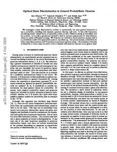
√ Combining with (2) and setting α = 100(c + M) ln ((c + M)t/ε) /t completes the proof. 4.3. Computation Time of Algorithm Aε . We now describe how the predictions of Aε are made efficiently. Let σt = x1 , x2 , . . . , xt−1 be the sequence formed by the first t − 1 rounds in the second stage, where xi , for 1 ≤ i < t, is the resource use time seen in round i. Recall from Section 3 that, for the tth round, algorithm Aε needs to output a strategy b j that has minimum cost on the rounds in σt . Any updates to the data structures used by algorithm Aε need to be made efficiently. We now describe a data structure maintained by algorithm Aε that allows predictions to be output in O(1) time and updates to be made in O(min{xt , c}/ε + log(c/ε)) time. (Note that in problems of interest, c ¿ M.) Algorithm Aε maintains the different candidate cutoffs as leaves of a balanced tree T . (See Figure 1.) We label the root of the tree by λ, and the leaves of the tree from left to right as 0 · · · v, such that the jth leaf corresponds to the cutoff b j . (For simplicity, we use the name b j for leaf j.) Let T (x) be the subtree of T rooted at node x, and let P(x) be the path from the root to (and including) node x. In particular, T is T (λ). With each (leaf and internal) node x, algorithm Aε maintains three variables, diff (x), min cost(x), and min cutoff (x). The algorithm maintains the following invariants for all t before the tth round. (These invariants define the variables.) We refer to the total cost of an algorithm that repeatedly uses a given cutoff over a sequence of resource use times as the cost of that cutoff on the sequence. The cost of using cutoff b j for σt is proportional to the sum of the diff values of the nodes in Pthe path from the root to b j , i.e., the cost of using cutoff b j for σt is proportional to x∈P(bj ) diff (x). The variable min cutoff (x) is the cutoff b j with minimum cost for σt amongst all cutoffs that are

44

P. Krishnan, P. M. Long, and J. S. Vitter

Fig. 1. Snapshot of the data structure used by algorithm Aε . In the situation depicted above there are eight candidate cutoffs labeled b0 , . . . , b7 , appearing as leaves of the tree. The value xt falls between b1 and b2 . The path P(b1 ) is shown with dotted lines. The diff values of all nodes marked with a “∗” are increased by the value of the cutoff at the node plus c. The diff values of the nodes marked with a “#” are increased by xt . The min cutoff and min cost values of all marked nodes (whether marked with a “∗,” “#,” or “+”) are updated.

leaves of T (x). The variable min cost(x) is closely related to the cost of the best cutoff amongst the leaves of T (x); in particular, it is the cost of the best cutoff amongst the leaves of T (x) minus the sum the nodes in P(parent(x)). Formally, P of the diff values ofP min cost(x) = minbl ∈T (x) { 1≤i 2 then discard current Aε , if one exists; set current Aε to be A1/2i endif feed resource use time xt to each active Aε end end At any sufficiently large time t, there are at most three active Aε ’s; i.e., if 4i ≤ t < 4i+1 , the active Aε ’s are A1/2i , A1/2i+1 , and A1/2i+2 . Hence, the space used by algorithm L is at most three times the√space used by algorithm A1/2i+2 , which we know from Section 4.1 is O(c/2i ) = O(c t). In round t, 4i ≤ t < 4i+1 , algorithm A1/2i has seen at least · 4i examples in its second stage; from Theorem 3, algorithm A1/2i is 4i − 4i−2 = 15 16 away from optimal by at most ! Ãr r ln(t (c + M)/2i ) ln t 1 . + k1 (c + M) =O 2i 15 · 4i−2 t The update time bound follows from Section 4.3.

46

P. Krishnan, P. M. Long, and J. S. Vitter

5.2. Algorithm L s . Algorithm L s is exactly Aε , with ε set appropriately such that s = B + v + max{η1 , η2,1 }. (See Section 4.1.) Since ε = 2(c/s), Theorem 2 follows from the discussion in Section 4. The lower bound on s arises from ε being suitable.

6. Adaptive Disk Spindown via Rent-to-Buy. As described in Section 1, the disk spindown scenario can be modeled as a rent-to-buy problem, where spinning the disk is equivalent to renting, and a spindown is equivalent to a buy. If energy conservation were the sole consideration of a disk spindown algorithm, the cost of a buy, c, is the ratio of the energy required to spindown the disk and spin it back up versus the power to keep the disk spinning. In practice, there are two conflicting goals of a disk spindown policy: conserving energy and preserving response time performance. In adaptive disk spindown, the user specifies the relative importance a of latency with respect to conserving energy, and the cost of the increased latency is integrated into c, the cost of the buy. We now describe precisely how this is done. Let Ps be the power consumed by a spinning disk. Typically, a spundown disk consumes Psd > 0 power, where Psd is much smaller than Ps . Let T be the net idle time at disk.7 This implies that the disk would consume at least T · Psd energy independent of the disk spindown algorithm. While comparing disk spindown algorithms for how well they do in terms of energy consumed, it is instructive to compare the excess energy, E X , consumed by a disk while using spindown algorithm X ; we define E X as the total energy consumed by algorithm X minus T · Psd . (This is essentially equivalent to saying that the power for keeping the disk spinning is Ps − Psd , and the power consumed by a spundown disk is zero.) The response time delay incurred while waiting for a spinup is proportional to the amount of time required to spinup a spundown disk. A natural measure of the net response time delay is, therefore, the number of operations that are delayed by a spinup. (Other measures of response time delay are possible as discussed in Section 7.2.5, item 4.) In adaptive disk spindown, the user specifies a parameter a, the relative importance of latency with respect to conserving energy. Let O X be the number of operations delayed by a spinup for algorithm X . Given a disk (spindown) management algorithm X , and a user specified parameter a, we define EC X , the effective cost of algorithm X , as (4)

EC X = E X + a · O X .

The goal of the disk spindown algorithm is to minimize the effective cost. The effective cost models the tradeoff between energy and response time in a natural fashion. In particular, a small value of a implies that energy conservation is the more important activity, while a larger value of a implies that response time is more critical. Minimizing effective cost can be modeled in the rent-to-buy scenario thus. Given the relative importance a, we determine the buy cost c. By definition, the value of c is the ratio of the effective cost for a spindown versus the effective cost per unit time to keep the disk spinning. Since a spindown delays one operation, the effective cost of 7 We assume that operations are synchronous, and that every algorithm sees the same sequence of idle times at disk. If this is not true, T can be defined as the minimum taken over all algorithms of the net idle time at disk.

Adaptive Disk Spindown via Optimal Rent-to-Buy in Probabilistic Environments

47

a spindown is E sd + a, where E sd is the total energy consumed by a spindown and a spinup. The effective cost per unit time to keep the disk spinning is Ps − Psd . Hence, c = (a + E sd )/(Ps − Psd ). For a given disk, the buy cost c is linearly related to the relative importance parameter a.

7. Experimental Results. In this section we describe the results of simulating our algorithm8 L from Section 5.1 for the disk spindown problem. We first describe the methodology used in our simulations and then describe the results of the simulation. 7.1. Methodology. We simulated algorithm L using a disk access trace from a HewlettPackard 9000/845 personal workstation running HP-UX. This trace is described in [18], and a portion of this trace was also used in a previous study of disk spindown policies [4]. The trace was obtained by Ruemmler and Wilkes by monitoring the disk for roughly 2 months; it consisted of 416,262 accesses to disk. We studied our algorithm for two disks, the Kittyhawk C3014A and the Quantum Go•Drive. The characteristics of the two drives are given in Table 1. (This table is derived from [4].) For our studies, we merged the active and idle states of the disk into one active state; notice that a disk can read and write data only in the active state. By merging these two states we ensure that a “buy” corresponds to a spindown. As in [4], we assumed that a disk access takes the average time for seek and rotational latency. We also assumed that all operations and state transitions take the average or “typical” time specified by the manufacturer, if one is specified, or else the maximum time. It is difficult to determine from a disk access trace why a specific access arrived at disk. We assumed that, if the disk is spundown, the application waits for the disk to spinup and complete the requested operation, and then performs the same sequence of operations as in the original system. In other words, although our simulations used disks that were different from the one on which the trace was collected, in our simulator we maintained the interarrival time of events at disk as in the original trace: if, in the original trace, Table 1. Disk characteristics of the Kittyhawk C3014A and Quantum Go•Drive 120. (This table appears in [4].)

Characteristic Capacity (Mbytes) Power consumed, active (W) Power consumed, idle (W) Power consumed, spundown (W) Power consumed, spinup (W) Normal time to spinup (s) Normal time to spindown (s) Average time to read 1 Kbyte (ms)

8

Hewlett-Packard Kittyhawk C3014A 40 1.50 0.62 0.27 2.17 1.10 0.55 22.50

Quantum Go•Drive 120 120 1.65 1.00 0.20 5.50 2.50 6.00 26.7

Instead of scheduling a new Aε at t ≈ 4i , in our simulations we scheduled a new Aε at t ≈ 2i .

48

P. Krishnan, P. M. Long, and J. S. Vitter

the tth access at disk arrived 1 seconds after the (t − 1)th access, in our simulation, we assumed that the tth access arrived 1 seconds after the (t −1)th access was completed by the disk. The basic problem with any strategy is that data dependency between different operations cannot be derived from the trace. We performed simulations for different values of a, the relative importance of response time to energy. For each a, we computed the buy cost c using the strategy described in Section 6. We compared our algorithm L against the following on-line algorithms: the two-competitive algorithm, which spins down the disk after c seconds of inactivity, and fixed-threshold policies that spindown the disk after 5 seconds, 30 seconds, and 5 minutes of inactivity; we also compared algorithm L against the optimal off-line rentto-buy algorithm, which knows the future and spins down the disk immediately if the next access is to take place more than c seconds in the future. For each algorithm X , we computed E X , the excess energy consumed, O X , the number of operations delayed by a spinup; from these values we computed EC X , the effective cost of algorithm X , using (4). For the HP trace, the maximum interarrival time was 1770.4 seconds; the maximum a we used corresponded to a c of 1770.4. 7.2. Results. In this section we present the results of our simulations. We first see how the effective cost varies with parameter a, and then look at how excess energy and number of operations delayed vary with a. Recall that the parameter a is linearly related to the buy cost c. In particular, for the Kittyhawk disk, c = 2.54 + a/1.225, and for the Go•Drive, c = 10.33 + a/1.45. The discussion from Section 6 implies that algorithm L and the 2-competitive algorithm try to optimize for effective cost as defined by (4). In particular, for really small values of a, algorithm L will essentially try to reduce excess energy, and for really large values of a, algorithm L will essentially try to reduce number of operations delayed. 7.2.1. Effective Cost versus a. Figures 2 and 3 show how the effective cost varies with parameter a using the Kittyhawk and Go•Drive disks, respectively. Each figure plots the curves for all values of a, and a clearer view for when a is small. We observe that algorithm L performs best amongst the on-line algorithms for (almost) all values of a. (It is roughly 1% worse than the 5-second threshold for a lying between 18 and 34 while using the Kittyhawk disk, and for a lying between 14 and 28 while using the Go•Drive.) In particular, the effective cost for algorithm L is 6–25% less than the effective cost of the 2-competitive algorithm (except for a small range of values of a between 34 and 60 with the Kittyhawk disk and for a between 28 and 58 for the Go•Drive when the effective costs for the two algorithms are roughly the same). As should be expected, each fixed threshold algorithm performs well for a very limited range of values for a. Interestingly, the 5-second threshold for certain small values of a and the 5-minute threshold for certain large values of a performs better than the 2-competitive algorithm. 7.2.2. Excess Energy versus a. As discussed in Section 6, when a is small, conserving energy is more important. Figure 4 plots the variation of excess energy with a using the Kittyhawk and Go•Drive disks for the various algorithms. We observe that for small values of a, algorithm L has the smallest excess energy amongst all on-line algorithms. In fact, it does better than the 5-second threshold, and

Adaptive Disk Spindown via Optimal Rent-to-Buy in Probabilistic Environments

49

Fig. 2. Variation of effective cost with a for the Kittyhawk disk. Part (b) zooms the portion of the graph for small values of a. The effective cost of the 5-minute threshold is comparatively high (the curve lies above 2,240,000), and is omitted from (b).

50

P. Krishnan, P. M. Long, and J. S. Vitter

Fig. 3. Variation of effective cost with a for the Go•Drive disk. Part (b) zooms the portion of the graph for small values of a. The effective cost of the 5-minute threshold is comparatively high (the curve lies above 2,700,000), and is omitted from (b); similarly, the curves for the 5-second and 30-second policies have been cropped at smaller values of a to show the details of the other three curves.

Adaptive Disk Spindown via Optimal Rent-to-Buy in Probabilistic Environments

51

Fig. 4. Variation of excess energy with a for the Kittyhawk and Go•Drive disks. The excess energy of the 5-minute threshold using the Kittyhawk disk is 2249 KJ, and using the Go•Drive is 2708 KJ; the curves for the 5-minute threshold are omitted from the graphs.

52

P. Krishnan, P. M. Long, and J. S. Vitter

its curve is almost parallel to the curve for the optimal off-line algorithm. In particular, algorithm L saves 17–60% more excess energy compared with the 2-competitive algorithm, and 6–42% more excess energy compared with the 5-second spindown threshold for small values of a (i.e., a < 25). We also observe that for small values of a, the 5-second threshold does better than the 2-competitive algorithm in terms of saving excess energy. (From Figures 2 and 3, we observe that, for most of these values of a, the 5-second threshold is also better than the 2-competitive algorithm in terms of effective cost.) 7.2.3. Operations Delayed versus a. As discussed in Section 6, when a is large, we want to reduce the number of operations delayed. Figure 5 plots the variation of number of operations delayed with a using the Kittyhawk and Go•Drive disks for the various algorithms. We observe two interesting phenomenon: first, the curves for the 2-competitive algorithm and the optimal off-line algorithm coincide for a large range of values for a. Second, algorithm L reduces the number of operations delayed over both these algorithms for sufficiently large a. 7.2.4. Adaptability and Rent-to-Buy. A different way of viewing the tradeoff between excess energy and response time is presented in Figure 6. In this figure excess energy is plotted as a function of number of operations delayed, and the different points on the curve are obtained by varying a; in particular, the value of a (or equivalently, c) decreases from left to right along the curve. (The curve for the Go•Drive is similar in shape and is omitted.) Figure 6 clearly shows the tradeoff between excess energy and response time obtained by varying a. We observe that by increasing the value of one parameter a (equivalent to varying the value of the buy cost c), we can effectively trade power for response time. Concerns on how to trade power for response time effectively have been raised for the disk spindown problem [3], [4], and the rent-to-buy model provides an elegant way of achieving this tradeoff. 7.2.5. Other Observations. lows:

Some other observations from our simulations are as fol-

1. As mentioned in Section 7.2.2, energy conservation is crucial when a is small, and algorithm L is best amongst the on-line algorithms in terms of excess energy for small a. Interestingly, we observed that the excess energy of algorithm L is less than the excess energy of the 2-competitive algorithm for all values of a. 2. We also compared our algorithm L against L s allowing at most 25 potential cutoffs for algorithm L s . Not surprisingly, algorithm L performed better than algorithm L s ; however, preliminary results suggest that algorithm L typically saved only 2–5% more excess energy than algorithm L s . Allowing more potential cutoffs for algorithm L s might help. 3. In our simulations, we used at most 300 cutoffs for our algorithm L. The computation time for the algorithm was therefore minimal. Interestingly, algorithm L did not change its cutoffs too often in stage 2. (The cutoff changed between 14 and 56 times when measured over all values of a.)

Adaptive Disk Spindown via Optimal Rent-to-Buy in Probabilistic Environments

53

Fig. 5. Variation of the number of operations delayed with a for the Kittyhawk and Go•Drive disks. The curves for the 2-competitive algorithm and the optimal off-line algorithm coincide for a large range of values of a.

54

P. Krishnan, P. M. Long, and J. S. Vitter

Fig. 6. Excess Energy, E L , as a function of the number of operations delayed, O L , for algorithm L. The graph was obtained by varying a (i.e., c); the value of a increases along the curve from left to right.

4. For measuring response time performance, we used the metric of the number of operations delayed. An alternative measure of response time performance is R X , the number of read operations delayed by a spinup for algorithm X [4]. This metric redefines the effective cost from (4) as E + a · R X . The rent-to-buy model can be easily modified to evaluate this measure, by having different costs for a spindown (i.e., different c’s) depending on whether the operation is a read or a write. We plan to consider the effect of this modification to the rent-to-buy cost in future work. For purely comparison purposes, Figure 7 plots the number of reads delayed as a function of a for the different algorithms; the algorithms are still optimizing for effective cost as defined by (4). (In other words, the rent-to-buy algorithms think they are optimizing for number of operations delayed, while we measure the number of reads delayed.) Interestingly, the curves from Figure 7 are similar to the corresponding curves from Figure 5(a), suggesting that we should expect to obtain similar results as presented in this paper by using the number of reads delayed metric instead of the number of operations delayed metric, when we modify the definition for effective cost appropriately.

8. Conclusions. In this paper we have looked at the problem of a sequence of unit rentto-buy choices where the resource use times are independently drawn from an unknown probability distribution. We have described how important systems problems (like the disk spindown problem in mobile machines) can be modeled by a rent-to-buy framework.

Adaptive Disk Spindown via Optimal Rent-to-Buy in Probabilistic Environments

55

Fig. 7. Number of reads delayed as a function of a for the various algorithms, while the rent-to-buy algorithms are optimizing using the definition of effective cost from (4). This graph is purely for illustration and comparison with Figure 5(a.) See Section 7.2.5, Item 4.

For the rent-to-buy problem, we have looked at computationally efficient strategies whose expected cost for the tth resource use converges to optimal as t → ∞ for any bounded probability distribution on the resource use times. We have also looked at a fixed-space algorithm which almost converges to optimal. We are currently looking at modeling the resource use times as being generated by a Hidden Markov Model (HMM) and have optimality results for special types of HMMs. Recently, Markov models have been effectively used to analyze caching and prefetching algorithms assuming user requests to pages in cache are generated by Markov sources [9], [12], [22]. Simulations of our algorithm for the disk spindown problem using disk access traces obtained from HP suggest that the rent-to-buy model is a good way to study disk spindown and related systems issues; in particular, a single parameter c effectively models the tradeoff between power and response time. We also introduced the new metric of “excess energy” that really reflects the relative performance in terms of energy consumed of one disk spindown algorithm against another. We introduced a natural notion of “effective cost” that incorporates the two metrics of excess energy, and number of operations delayed weighted by a user-specified parameter a, into one cost. We observed that our algorithm L out-performed other on-line algorithms in terms of effective cost for almost all values of a; in particular, it had 6–25% less effective cost than the 2-competitive algorithm. In addition, for small values of a (corresponding to when saving energy is critical), we observed that our algorithm L saves 17–60% more of excess energy compared with the 2-competitive algorithm, and 6–42% more excess energy compared with the 5-second fixed threshold.

56

P. Krishnan, P. M. Long, and J. S. Vitter

Acknowledgments. We thank John Wilkes and the Hewlett-Packard Company for making their file system traces available to us. We thank Peter Bartlett for his comments, and Fred Douglis for his comments and interesting discussions related to the disk spindown problem. References [1] A. Blumer, A. Ehrenfeucht, D. Haussler, and M. K. Warmuth, Learnability and the Vapnik–Chervonenkis Dimension, Journal of the ACM (October 1989). [2] L. Devroye, L. Gyorfi, and G. Lugosi, A Probabilistic Theory of Pattern Recognition, Springer-Verlag, New York, 1996. [3] F. Douglis, P. Krishnan, and B. Bershad, Adaptive Disk Spindown Policies for Mobile Computers, Computing Systems 8 (1995). [4] F. Douglis, P. Krishnon, and B. Marsh, Thwarting the Power Hungry Disk, Proceedings of the 1994 Winter USENIX Conference (January 1994). [5] P. Greenwall, Modeling Power Management for Hard Disks, Proceedings of the Symposium on Modeling and Simulation of Computer Telecommunication Systems (1994). [6] D. P. Helmbold, D. D. E. Long, and B. Sherrod, A Dynamic Disc Spin-down Technique for Mobile Computing, Proceedings of MOBICOM ’96. [7] A. R. Karlin, K. Li, M. S. Manasse, and S. Owicki, Empirical Studies of Competitive Spinning for a Shared-Memory Multiprocessor, Proceedings of the 1991 ACM Symposium on Operating System Principles (1991). [8] A. R. Karlin, M. S. Manasse, L. A. McGeoch, and S. Owicki, Competitive Randomized Algorithms for Non-Uniform Problems, Proceedings of the 1st ACM–SIAM Symposium on Discrete Algorithms (1990). [9] A. R. Karlin, S. J. Phillips, and P. Raghavan, Markov Paging, Proceedings of the 33rd Annual IEEE Conference on Foundations of Computer Science (October 1992). [10] M. J. Kearns and R. E. Schapire, Efficient Distribution-Free Learning of Probabilistic Concepts, Proceedings of the 31st Annual IEEE Symposium on Foundations of Computer Science (October 1990). [11] S. Keshav, C. Lund, S. J. Phillips, N. Reingold, and H. Saran, An Empirical Evaluation of Virtual Circuit Holding Time Policies in IP-over-ATM Networks, Proceedings of INFOCOM ’95. [12] P. Krishnon and J. S. Vitter, Optimal Prediction for Prefetching in the Worst Case, SIAM Journal on Computing, to appear. An extended abstract appears in Proceedings of the 5th Annual ACM–SIAM Symposium on Discrete Algorithms, January 1994. [13] K. Li, R. Kumpf, P. Horton, and T. Anderson. A Quantitative Analysis of Disk Drive Power Management in Portable Computers, Proceedings of the 1994 Winter USENIX (January 1994). [14] C. Lund, S. Phillips, and N. Reingold, IP over Connection-Oriented Networks and Distributed Paging, Proceedings of the 35th Annual IEEE Symposium on Foundations of Computer Science (November 1994). [15] B. Marsh, F. Douglis, and P. Krishnan, Flash Memory File Caching for Mobile Computers, Proceedings of the 27th IEEE Hawaii Conference on System Sciences (January 1994). [16] Hewlett Packard, Kittyhawk HP C3013A/C3014A Personal Storage Modules Technical Reference Manual, March 1993, HP Part No. 5961-4343. [17] D. Pollard, Convergence of Stochastic Processes, Springer-Verlag, New York, 1984. [18] C. Ruemmler and J. Wilkes, UNIX Disk Access Patterns, Proceedings of the 1993 Winter USENIX Conference (January 1993). [19] H. Saran, and S. Keshav, An Empirical Evaluation of Virtual Circuit Holding Times in IP-over-ATM Networks, Proceedings of INFOCOM ’94 (June 1994). [20] V. N. Vapnik, Inductive Principles of the Search for Empirical Dependences (Methods Based on Weak Convergence of Probability Measures), Proceedings of the 1989 Workshop on Computational Learning Theory (1989). [21] V. N. Vapnik and A. Y. Chervonenkis, On the Uniform Convergence of Relative Frequencies of Events to Their Probabilities, Theoretical Probability and Its Applications 16 (1971), 264–280. [22] J. S. Vitter and P. Krishnan, Optimal Prefetching via Data Compression, Journal of the ACM 43 (September 1996), 771–793.