Efficient Data Stream Classification via Probabilistic Adaptive Windows
Recommend Documents
Smaller values of GP3 (line 6, Algorithm 1) causes recalculations of the split heuristic ..... ing scenario since instances are sequentially presented as a time series [3]. This data set ...... online boosting. pages 2323â2331, 2015. 9. Albert Bife
Dayong Wangâ, Pengcheng Wuâ , Peilin Zhaoâ¡, Yue Wu§, Chunyan Miaoâ and Steven C.H. Hoiâ . âSchool of Computer Engineering, Nanyang Technological ...
S.M.Aqil Burney. M.Sadiq Ali Khan. Mr.Jawed Naseem. Department of Computer Science. Department of Computer Science. Principal Scientific Officer-PARC.
Incremental Parallel Random Forest (IPRF) algorithm for data streams in ... proposed mechanism using benchmark datasets are presented in this paper. .... massive distributed processing of datasets, receives input data streams, divides the data into b
Aug 1, 2014 - Our visual analysis tools: (a) the confusion wheel shows ...... visual analytics system for classification based on supervised dimension reduction.
Feb 22, 2018 - Sanket Kamthe, Marc Peter Deisenroth to the RBF policy. This allows ...... Press, 2003. [27] A. Y. Ng and M. I. Jordan. PEGASUS: A Policy.
Data stream classification and big data analytics. Nowadays, the development of computers technology and its recent applications provide access to new types ...
Adaptive XML Stream Classification using Partial Tree-edit Distance. Dariusz Brzezinski and Maciej Piernik. Institute of Computing Science, Poznan University of ...
Dec 13, 2005 - To facilitate understanding and support for steelhead conservation, management and recovery strategies. D
An Adaptive Energy-Efficient Stream Decoding. System for Cloud Multimedia Network on Multicore Architectures. Chin-Feng Lai, Member, IEEE, Ying-Xun Lai, ...
was adjusted to reduce the cloud multimedia data dependence by dynamic-voltage-frequency-scaling system. The adaptive energy- efficient stream decoding ...
Abstract. In the single rent-to-buy decision problem, without a priori knowledge of the amount of time a resource will be used we need to decide when to buy the ...
Jul 28, 2014 - discriminant analysis (PLDA), single SVM, classification and regression trees ... An R/BIOCONDUCTOR package MLSeq with a vignette is freely available at ... bisulfite-sequencing data for DNA methylation profiling. ..... The same workfl
the limited network capacity for moving large datasets. A tool that addresses this challenge is the Bulk Data Mover. (BDM), a data transfer management tool used ...
Dynamic Time Warping (DTW) similarity to acclimate its rate of sampling according to ...... Mouftah, HT (2011) 'The internet of things', IEEE. Commun. Mag, Vol.
ing search engines. Query classification is a task studied for this purpose. In query classification, user queries are clas- sified into one (or more) predefined target ...
Nov 3, 2015 - At the same time, gradient descent methods are becoming ... This gradient nature of the algorithm makes it suitable to be trained in- crementally ...
For the classification task on uncertain data, a few decision tree algorithms have been proposed [1 ... in attribute values by probability distribution functions (pdf). ..... Jenhani, I., Amor, N.B., Eluouedi, Z.: Decision trees as possibilistic clas
Nov 3, 2015 - Big Data streams are being generated in a faster, bigger, and more common- ... Keywords: Data Stream Mining, Big Data, Classification, GPUs.
click-stream analysis, market basket data mining, fraud detection etc.,. Therefore, the processing of data streams needs i) To examine each data element of data ...
fiers and applies automatic updating of ensemble models for han- ..... [7] C. W. Mohammad M. Masud, Jing Gao, Latifur Khan, Jiawei Han,. Kevin W. Hamlen ...
Jan 19, 2012 - we present a hormone based nearest neighbor classification algorithm for data stream classification, in which the classi- fier is updated every ...
Efficient Data Stream Classification via Probabilistic Adaptive Windows
tic adaptive window (PAW) for data-stream learning, which improves ... measurements in network monitoring and traffic manage- ment ..... for θ = 9, 8, 7 and 9.5.
Efficient Data Stream Classification via Probabilistic Adaptive Windows Albert Bifet
Jesse Read
Yahoo! Research Barcelona Barcelona, Catalonia, Spain
Dept. of Signal Theory and Communications Universidad Carlos III Madrid, Spain
Dept. of Computer Science University of Waikato Hamilton, New Zealand
Dept. of Computer Science University of Waikato Hamilton, New Zealand
[email protected] ABSTRACT In the context of a data stream, a classifier must be able to learn from a theoretically-infinite stream of examples using limited time and memory, while being able to predict at any point. Many methods deal with this problem by basing their model on a window of examples. We introduce a probabilistic adaptive window (PAW) for data-stream learning, which improves this windowing technique with a mechanism to include older examples as well as the most recent ones, thus maintaining information on past concept drifts while being able to adapt quickly to new ones. We exemplify PAW with lazy learning methods in two variations: one to handle concept drift explicitly, and the other to add classifier diversity using an ensemble. Along with the standard measures of accuracy and time and memory use, we compare classifiers against state-of-the-art classifiers from the data-stream literature.
1.
INTRODUCTION
The trend to larger data sources is clear, both in the real world and the academic literature. Nowadays, data is generated at an ever increasing rate from sensor applications, measurements in network monitoring and traffic management, log records or click-streams in web exploration, manufacturing processes, call-detail records, email, blogs, RSS feeds, social networks, and other sources. Real-time analysis of these data streams is becoming a key area of data mining research as the number of applications demanding such processing increases. A data stream learning environment has different requirements from the traditional batch learning setting. The most
Permission to make digital or hard copies of all or part of this work for personal or classroom use is granted without fee provided that copies are not made or distributed for profit or commercial advantage and that copies bear this notice and the full citation on the first page. To copy otherwise, to republish, to post on servers or to redistribute to lists, requires prior specific permission and/or a fee. SAC’13 March 18-22, 2013, Coimbra, Portugal. Copyright 2013 ACM 978-1-4503-1656-9/13/03 ...$15.00.
significant are the following, as outlined in [1]: • process one example at a time, and inspect it only once (at most); • be ready to predict (a class given a new instance) at any point; • adapt to data that may evolve over time; and • expect an infinite stream, but process it under finite resources (time and memory). Proper evaluation of the performance of algorithms in a stream environment is a major research question. Up to now the focus has mainly been on developing correct procedures for comparing two or more classifiers with respect to their predictive performance. In practice, finite resources limit the choice of algorithms that can actually be deployed; we need to gauge at least approximately how much predictive performance can be obtained given the investment of computational resources. Therefore we argue for the inclusion of time and memory usage as dimensions in the assessment of algorithm performance. Several methods from the literature incrementally record probabilistic information from each example they see in the stream to build an incremental model over time (for example, Naive Bayes, or Hoeffding Trees). Other methods maintain a “window” of examples to learn from (for example k-Nearest Neighbour (kNN), nearest centroid (Rocchio) classifiers, and other lazy methods). A basic implementation will maintain a sliding window of a fixed size. It is not possible to store of all stream instances due to eventual memory (and processing) limitations. Despite the fact that the implementation is limited by the size of its sliding window, our analysis has revealed that such methods can be extremely competitive in a data-stream environment, not only in terms of predictive performance but also time and memory usage. They require very few training examples to learn a concept (many less than, for example, Hoeffding Trees) and their window provides a natural mechanism for handling concept drift; as it will contain the most recent instances – precisely the ones which are most likely to be relevant for the next prediction. The resulting classifier
needs to be tuned to the data stream in terms of the size of the window, but even relatively small windows provide surprisingly good performance. However, a weakness of this existing sliding-window approach is that it can forget too many old instances, as they are dropped from the window. While the most recent training instances are usually most likely to be the most relevant ones when making a prediction for a new instance, this is not always the case, and older instances may carry information that is still relevant, or may become relevant again in the future. Using our analysis, we introduce a new method for learning from data streams: Probabilistic Approximate Window (PAW). This method finds the compromise between the relevance of information in the most recent instances, and the preservation of information carried by older instances. PAW maintains a sample of instances in logarithmic memory, giving greater weight to newer instances. But rather than leaving the window to naturally adapt to the stream we use an explicit change detector and keep only those instances that align with the most recent distribution of the data. Additionally, since it has been shown previously [2] that adding classifier diversity can significantly boost the performance of a base classifier, we also investigate the accuracy gains of deploying this leveraging bagging for our k-Nearest Neighbour method. This paper is structured as follows. Section 2 details prior work that we draw on for comparison. We introduce the Probabilistic Approximate Window method and its two variations in Section 3. Section 4 then details the data sets used and the results of comparing the three lazy learning methods with state-of-the-art base and ensemble classifiers. Finally, we make concluding remarks in Section 6 and indicate avenues for future research on these methods.
2.
PRIOR WORK
Naive Bayes [3] is a widely known classifier; it simply updates internal counters with each new instance and uses these counters to assign a class to an unknown instance probabilistically. Naive Bayes makes a good baseline for classification, but in terms of performance, has been superseded by Hoeffding Trees [4]: an incremental, anytime decision tree induction algorithm that is capable of learning from massive data streams by exploiting the fact that a small sample is often enough to choose an optimal splitting attribute. Hoeffding Trees have been shown to work particularly well in a Bagging ensemble [5, 2]. Unlike Naive Bayes and Hoeffding Trees, a k-Nearest Neighbour algorithm cannot learn from a stream indefinitely without discarding data, since it maintains an internal buffer of instances that it must search through to find the neighbours of each test instance. When the internal buffer fills up, it serves as a first-in-first-out sliding window of instances. The prediction of the class label of an instance is made using the majority vote of its k nearest neighbors from inside this window. Even though improved search [6] and instance-compression techniques [7] have been shown to improve its capacity considerably, the question of how to properly deal with kNN in a concept drift setting is still open. Recent work, such as [6] still only removes outdated instances when space is needed
for new instances, and they test their methods mainly on medium sized datasets. [8] also provides a fast implementation of k-Nearest Neighbour, but this work is focussed on automatically calibrating the number of neighbours k and does not consider data with concept drift. Reacting to concept drift is a fundamental part of learning from data streams [9]. As previously mentioned, k-Nearest Neighbour methods do this to some extent automatically, as they are forced to phase out part of their model over time due to resource limitations; nevertheless it is possible to add an explicit change detection mechanism. ADWIN [10], which keeps a variable-length window of recently seen items (such as the current classification performance), is an example of this, and has been used successfully with Hoeffding Trees [5]. Our experimental evaluation reveals that kNN methods perform surprisingly well. This has an important implication: that it is not necessary to learn from all instances in a stream to be competitive in data-stream classification.
3.
PROBABILISTIC APPROXIMATE WINDOWS (PAW)
In the dynamic nature of data streams, more recent examples tend to be the most representative ones of the current concept. Nevertheless, forgetting too many old instances will result in reduced accuracy, as too much past information disappears, leaving the learner with a small snapshot of part of the current concept. A classifier, therefore, should aim to learn as quickly as possible from new examples, but also maintain some information from older instances. We propose a new methodology which does exactly this by maintaining in logarithmic memory a sample of the instances, giving more weight to newer ones. Rather than storing all instances or only a limited window, the Probabilistic Approximate Window algorithm (PAW) keeps a sketch window, using only a logarithmic number of instances, storing the most recent ones with higher probability. It draws inspiration from the Morris approximate counting algorithm, which was introduced in what is considered to be the first paper on streaming algorithmics [11]. The main motivation of this counting algorithm, is how to store in 8 bits, a number larger than 28 = 256. Suppose that we have a stream of events or elements, and we want to count its number of events n using only a counter of 8 bits. The idea of the method is simple, instead of storing n using log(n) bits, it is possible to store its logarithm using log(log(n)) bits. Algorithm 1 Morris approximate counting 1 2 3 4 5
Init counter c ← 0 for every event in the stream do rand = random number between 0 and 1 if rand < p then c ← c + 1
Algorithm 1 shows the pseudocode of the algorithm. Basically, for each new event that arrives, it decides with probability p if it updates the counter c by one. The error and the variance of the estimation depends on the probability p chosen.
10
Algorithm 2 Probabilistic Approximate Window
8
Probabilistic Approximate Window 1 Init window w ← ∅ 2 for every instance i in the stream 3 do store the new instance i in window w 4 for every instance j in the window 5 do rand = random number between 0 and 1 6 if rand > b−1 7 then remove instance j from window w
6 4 2 0
0
2
4
6
8
10
x 100 dow, but not the window itself. PAW extends it to keep the window of elements using logarithmic memory. The algorithm works as follows: when a new instance of the stream arrives, it is stored in the window. Then, each single instance in the window is up for randomized removal, with a probability of 1 − b−1 . We use the setting proposed by Flajolet: b = 2−1/w where w is a parameter value related to the size of the sketch window that we would like to keep.
80 60 40 20 0
0
20
40
60
80
100
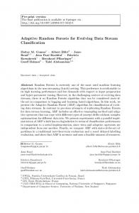
x Figure 1: Probability function used by Morris to store counts for a = 30: f (x) = log(1 + x/30)/ log(1 + 1/30); plotted up to x = 10 (top) and x = 100 (bottom). The first values are stored with higher probability and the rest with lower probability.
Let us see a simple case: for each event that arrives in the stream, the algorithm decides, randomly with p = 1/2, if it updates the counter c by one or not. The counter will maintain an estimate of the number of items arrived divided by two. The variance is σ 2 = np(1 − p) = n/4 as p = 1/2. For example, imagine that we have 400 events, the counter will maintain a count p of c = n/2 = 200, and the standard deviation will be σ = n/4, i.e. σ = 10 for this case. Morris proposed to store in the register the value given by the function f (x) = log(1 + x/a)/ log(1 + 1/a). Figure 1 shows for a = 30 how the first 10 values stored are similar to the real ones, but for values after the 10th element, the values follow a logarithmic law. Choosing p = 2−c where c is the value of the counter that we are maintaining, Flajolet [12] proved that we get an estimation E[2c ] = n + 2 and a variance of σ 2 = n(n + 1)/2. A way to improve the variance using the same amount of space, is using a base b smaller than 2 in the logarithms. Then p = b−c , the estimation is E[bc ] = n(b−1)+b, the value of the counter is n = E[(bc − b)/(b − 1)] and the variance is σ 2 = (b − 1)n(n + 1)/2. For example, suppose that we have 8 bits to store our counter, and b = 2. The maximum value stored is √ 2255 − 1 and the standard deviation is approximately 2255 / 2. Instead, if we use b = 21/16 then we reduce the variance to a twentieth part, since b − 1 = 0.044. Algorithm 2 shows the pseudocode of the Probabilistic Approximate Window algorithm (PAW). Morris approximate counting can be used to store the size of a win-
Proposition 1. Given a data stream of items i1 , i2 , i3 , . . . , it , . . . , the Probabilistic Approximate Window algorithm maintains a window data structure with the following properties: • Given b = 2−1/w , the probability pn of having item in stored in the window, after receiving a further m items, is pm−n = 2−(m−n)/w • An estimate of the size of the window W after receiving m items is given by (1 − 2−(m+1)/w )/(1 − 2−1/w ) • An estimate of the size of the window W to maintain an infinite stream is given by 1/(1 − 2−1/w ) We omit proofs here, as they are straightforward from Flajolet’s work. We further improve the method in two ways: 1. We add concept-drift adaptive power, using a change detector to keep only the examples that correspond to the most recent distribution of the data. We use ADWIN [10], since it is a change detector and estimator that solves, in a well-specified way, the problem of tracking the average of a stream of bits or real-valued numbers. ADWIN keeps a variable-length window of recently seen items, with the property that the window has the maximal length statistically consistent with the hypothesis “there has been no change in the average value inside the window”. ADWIN maintains its own window in a compressed fashion, using only O(ln(w)) space for a window of size w. 2. We add diversity using a leveraging bagging method [2] to improve accuracy, creating classifiers using different random instances as input. First, we initialize n classifiers. For each new instance that arrives, we train each classifier with a random weight of P oisson(λ), where λ is a parameter chosen by the user. When a change is detected, the worst classifier of the ensemble of classifiers is removed and a new classifier is added to the ensemble. To predict the class of an example, we output as a prediction the class with the most votes.
4.
EXPERIMENTS
In this section we look at the performance offered by Probabilistic Adaptive Windowing (PAW). We exemplify PAW with the k Nearest Neighbour algorithm (kNN), using the PAW window as its sliding window. The prediction of a class label for each instance is made by taking the majority vote of its k nearest neighbors in the window. kNN has been shown to perform surprisingly well against a variety of other methods in the data-stream context [13, 14]. We compare the performance of our method (kNN with PAW) to existing well-known and commonly-used methods in the literature: Naive Bayes, Hoeffding Tree, Hoeffding Tree ensembles, and kNN using a standard windowing technique of the previous w examples. These methods, and their parameters, are displayed in Table 1. We also compare to kNN with the variations of PAW we described in Section 3. All algorithms evaluated in this paper were implemented in Java by extending the MOA software [15]. We use the experimental framework for concept drift presented in [1]: considering data streams as data generated from pure distributions, we can model a concept drift event as a weighted combination of two pure distributions that characterizes the target concepts before and after the drift. This framework defines the probability that a new instance of the stream belongs to the new concept after the drift based on the sigmoid function. Our experimental evaluation comprises two parts: 1. We study the effects of different batch-size parameters value for the k nearest neighbour methods; and then
Table 1: The methods we consider. Leveraging Bagging methods use n models. kNNWA empties its window (of max w) when drift is detected (using the ADWIN drift detector). Abbr.
Classifier
Parameters
NB HT HTLB kNN kNNW kNNWA kNNLB W
Naive Bayes Hoeffding Tree Leveraging Bagging with HT k Nearest Neighbour kNN with PAW kNN with PAW+ADWIN Leveraging Bagging with kNNW
n = 10 w = 1000, k = 10 w = 1000, k = 10 w = 1000, k = 10 n = 10
Table 2: The window size for kNN and corresponding performance. Accuracy −w 100 −w 500 −w 1000 −w 5000 Real Avg. Synth. Avg. Overall Avg.
77.88 57.99 62.53
77.78 81.93 80.28
79.59 84.74 82.59
78.23 86.03 83.11
Time (seconds) Real Tot. Synth. Tot. Overall Tot.
−w 100
−w 500
−w 1000
−w 5000
297 371 668
998 1297 2295
1754 2313 4067
7900 10671 18570
RAM Hours −w 100 −w 500 −w 1000
−w 5000
2. We compare the performance of all methods. We measure predictive performance (accuracy), running time, and RAM-Hours (as in [16] where one GB of RAM deployed for one hour equals one RAM-Hour).
4.1
Data
In our experiments we use a range of both real and synthetic data sources. Synthetic data has several advantages – it is easier to reproduce and there is little cost in terms of storage and transmission. For this paper we use the data generators most commonly found in the literature. SEA Concepts Generator An artificial dataset, introduced in [17], which contains abrupt concept drift. It is generated using three attributes. All attributes have values between 0 and 10. The dataset is divided into four concepts by using different thresholds θ; such that: f1 +f2 ≤ θ where f1 and f2 are the first two attributes, for θ = 9, 8, 7 and 9.5. Rotating Hyperplane The orientation and position of a hyperplane in d-dimensional space is changed to produce concept drift; see [18]. Random RBF Generator Using a fixed number of centroids of random position, standard deviation, class label and weight. Drift is introduced by moving the centroids with constant speed. LED Generator The goal is to predict the digit displayed on a seven-segment LED display, where each attribute has a 10inverted; LED comprises 24 binary attributes, 17 of which are irrelevant; see [19].
The UCI machine learning repository [20] contains some real-world benchmark data for evaluating machine learning techniques. We consider three of the largest: Forest Covertype Contains the forest cover type for 30 x 30 meter cells obtained from US Forest Service data. It contains 581, 012 instances and 54 attributes. It has been used in, for example, [21, 22]. Poker-Hand 1, 000, 000 instances represent all possible poker hands. Each card in a hand is described by two attributes: suit and rank. Thus there are 10 attributes describing each hand. The class indicates the value of a hand. We sorted by rank and suit and removed duplicates. Electricity Contains 45, 312 instances describing electricity demand. A class label identifies the change of the price relative to a moving average of the last 24 hours. It was described by [23] and analysed also in [9].
Table 3: Comparison of all methods. Accuracy∗ HT HTLB
NB CovType Elec. Poker Real avg. LED(5E5) SEA(50) SEA(5E5) HYP10 0.0001 HYP10 0.001 RBF00 RBF50 0.0001 RBF10 0.0001 RBF50 0.001 RBF10 0.001 Synth. avg. Overall avg ∗
The experiments were performed on 2.66 GHz Core 2 Duo E6750 machines with 4 GB of memory. The evaluation method used was Interleaved Test-Then-Train; a standard online learning setting where every example is used for testing the model before using it to train. This procedure was carried out on 10 million examples from the hyperplane and RandomRBF datasets, and one million examples from the SEA dataset. The parameters of these streams are the following:
• SEA(v): SEA dataset, with length of change v. • LED(v): LED dataset, with length of change v. The Nemenyi test [24] is used for computing significance: it is an appropriate test for comparing multiple algorithms over multiple datasets; it is based on the average ranks of the algorithms across all datasets. We use a p-value of 0.05. Under the Nemenyi test, x y indicates that algorithm x is statistically significantly more likely to be more favourable than y. Table 2 displays results for a variety of window sizes for kNN. It illustrates the typical trade-off for window sizes: too small a window can significantly degrade the accuracy of a classifier (see w = 100); whereas too large a window can significantly augment the running time and memory requirements (w = 5000). Our choice is for w = 1000. Using higher w, for example, w = 5000, can result in slightly better accuracy, but the improvement is in our opinion not significant enough to justify the massive increase in the use of computational resources. Table 3 displays the final accuracy and resource use (time and RAM-hours) of all the methods, as detailed in Table 1. Accuracy is measured as the final percentage of examples correctly classified over the test/train inter-leaved evaluation.
5.
DISCUSSION
The overall most accurate method is our PAW-based kNNLB W : a lazy method with a data-stream specific adaption for phasing out older instances, combined with the power of Leveraging Bagging. This method performs the best on average of all the methods in our comparison. The kNN methods perform much better than baseline Naive Bayes (NB) and even the reputed Hoeffding Tree (HT). This is noteworthy, since their models are restricted to a relatively small subset of instances (1000 in this case). HT is relatively more competitive on the real data. This is almost
certainly because the real data comprises relatively stable concepts (little drift) where Hoeffding Trees perform well. HTLB is relatively much more powerful; achieving relatively higher accuracy compared to HT and even proving competitive with kNN methods overall. However, this is at the price of being RAM Hours, orders of magnitude greater than HT, and over 14 times slower. It is comparable with the kNN methods insofar as time, but uses many more RAM Hours. When our kNNW method is applied under Leveraging Bagging (kNNLB W ) we also see a considerable increase in the use of computational resources. But with this trade off it performs best on over half of all datasets. Table 3 provides us with an interesting comparison of Naive Bayes, Hoeffding trees, Leveraging Bagging with Hoeffding Tress, and variations of kNN. Naive Bayes (NB) uses the least resources, but its accuracy is poor compared to all other methods; with the single exception of HYP(10,0.0001), for which it obtains the second-best score. As claimed in the literature, Hoeffding Trees (HT) are a better choice than NB for instance-incremental methods.
6.
CONCLUSIONS
In this paper we presented a probabilistic adaptive window method for window-based learning in evolving data streams, based on the approximate counting of Morris. Using this window approach we designed three methods: one that does not take into consideration concept drift explicitly, one that detects concept drift explicitly and removes instances that may be not corresponding to the actual distribution of data, and additionally an approach using leveraging bagging as an ensemble method to improve diversity. Our experimental evaluation – of real and synthetic data sources with different types and magnitudes of concept drift – justified the effectiveness of our probabilistic adaptive window; the lazy learning strategies we employed with this window obtained a high predictive performance to efficiency ratio over the comparison methods. In future work we intend to experiment with different distance metrics in our lazy methods, and investigate the performance gains of using our probabilistic adaptive window approach with other classification techniques.
7.
[6]
[7]
[8]
[9]
[10]
[11]
[12] [13]
[14]
[15]
[16]
[17]
[18]
REFERENCES [19]
[1] A. Bifet, G. Holmes, B. Pfahringer, R. Kirkby, and R. Gavald` a, “New ensemble methods for evolving data streams,” in KDD, 2009, pp. 139–148. [2] A. Bifet, G. Holmes, and B. Pfahringer, “Leveraging bagging for evolving data streams,” in ECML/PKDD (1), ser. Lecture Notes in Computer Science, J. L. Balc´ azar, F. Bonchi, A. Gionis, and M. Sebag, Eds., vol. 6321. Springer, 2010, pp. 135–150. [3] G. H. John and P. Langley, “Estimating continuous distributions in bayesian classifiers,” in Eleventh Conference on Uncertainty in Artificial Intelligence. San Mateo: Morgan Kaufmann, 1995, pp. 338–345. [4] P. Domingos and G. Hulten, “Mining high-speed data streams,” in KDD, 2000, pp. 71–80. [5] A. Bifet and R. Gavald` a, “Adaptive learning from evolving data streams,” in IDA, ser. Lecture Notes in Computer Science, N. M. Adams, C. Robardet,
[20] [21]
[22]
[23]
[24]
A. Siebes, and J.-F. Boulicaut, Eds., vol. 5772. Springer, 2009, pp. 249–260. P. Zhang, B. J. Gao, X. Zhu, and L. Guo, “Enabling fast lazy learning for data streams,” in ICDM, 2011, pp. 932–941. E. Spyromitros-Xioufis, M. Spiliopoulou, G. Tsoumakas, and I. Vlahavas, “Dealing with concept drift and class imbalance in multi-label stream classification,” in IJCAI, 2011, pp. 1583–1588. Y.-N. Law and C. Zaniolo, “An adaptive nearest neighbor classification algorithm for data streams,” in 9th European Conference on Principles and Practice of Knowledge Discovery in Databases, 2005, pp. 108–120. J. Gama, P. Medas, G. Castillo, and P. P. Rodrigues, “Learning with drift detection,” in SBIA, 2004, pp. 286–295. A. Bifet and R. Gavald` a, “Learning from time-changing data with adaptive windowing,” in SDM, 2007. R. Morris, “Counting large numbers of events in small registers,” Commun. ACM, vol. 21, no. 10, pp. 840–842, Oct. 1978. P. Flajolet, “Approximate counting: A detailed analysis,” BIT, vol. 25, no. 1, pp. 113–134, 1985. J. Read, A. Bifet, B. Pfahringer, and G. Holmes, “Batch-incremental versus instance-incremental learning in dynamic and evolving data,” in 11th Int. Symposium on Intelligent Data Analysis, 2012. A. Shaker and E. H¨ ullermeier, “Instance-based classification and regression on data streams,” in Learning in Non-Stationary Environments. Springer New York, 2012, pp. 185–201. A. Bifet, G. Holmes, R. Kirkby, and B. Pfahringer, “MOA: Massive Online Analysis http://moa.cs.waikato.ac.nz/,” JMLR, 2010. A. Bifet, G. Holmes, B. Pfahringer, and E. Frank, “Fast perceptron decision tree learning from evolving data streams,” in PAKDD, 2010. W. N. Street and Y. Kim, “A streaming ensemble algorithm (SEA) for large-scale classification,” in KDD, 2001, pp. 377–382. G. Hulten, L. Spencer, and P. Domingos, “Mining time-changing data streams,” in KDD, 2001, pp. 97–106. L. Breiman, J. H. Friedman, R. A. Olshen, and C. J. Stone, Classification and Regression Trees. Wadsworth, 1984. A. Asuncion and D. Newman, “UCI machine learning repository,” 2007. J. Gama, R. Rocha, and P. Medas, “Accurate decision trees for mining high-speed data streams,” in KDD, 2003, pp. 523–528. N. C. Oza and S. J. Russell, “Experimental comparisons of online and batch versions of bagging and boosting,” in KDD, 2001, pp. 359–364. M. Harries, “Splice-2 comparative evaluation: Electricity pricing,” The University of South Wales, Tech. Rep., 1999. J. Demˇsar, “Statistical comparisons of classifiers over multiple data sets,” The Journal of Machine Learning Research, vol. 7, pp. 1–30, 2006.