Adaptive Distributed Estimation over Wireless Sensor Networks with Packet Losses Alberto Speranzon
Carlo Fischione
Bj¨orn Johansson and Karl Henrik Johansson
Unilever R&D Port Sunlight Quarry Road East CH63 3JW Bebington United Kingdom
UC Berkeley Hearst Ave. 94720 Berkeley CA
School of Electrical and Engineering Royal Institute of Technology Osquldas v¨ag 10 100-44 Stockholm, Sweden
[email protected]
[email protected]
{bjorn.johansson|kallej}@ee.kth.se
Abstract—A distributed adaptive algorithm to estimate a time-varying signal, measured by a wireless sensor network, is designed and analyzed. The presence of measurement noises and of packet losses is considered. Each node of the network locally computes adaptive weights that guarantee to minimize the estimation error variance. Decentralized conditions on the weights, which ensure the stability of the estimates throughout the overall network, are also considered. A theoretical performance analysis of the scheme is carried out both in the presence of perfect and lossy links. Numerical simulations illustrate performance for various network topologies and packet loss probabilities. Index Terms—Distributed filtering; Wireless sensor networks; Networked Embedded System.
I. I NTRODUCTION The robustness, flexibility and reduced cost of Wireless Sensor Networks (WSNs) motivate the development of new classes of estimation algorithms, which need to be designed considering the limited computational and communication capabilities of such systems. Collaboration is suitable to overcome intrinsic limitations in processing measurements from only a single sensor, which often provide data with correlated data and quantization noise [1]. The main contribution of this paper is a theoretical framework to the design of a collaborative distributed filter for tracking a time-varying signal with a WSN. The approach ensures that the filter is stable and exhibits good behavior with respect to packet losses. We state and solve an optimization problem that provides optimal filter coefficients that guarantees the stability of the estimation error even in presence of lossy communications. The filter design is based on new global constraints, which are different from those adopted in the earlier work [2], [3]. Studies on the properties of distributed algorithm are found in the area of parallel computing [4]. More recently, they have found renewed interest in several other research areas, including communication networks, multi-robot coordination, and signal processing. Here we limit the discussion to some recent and relevant contributions. In [5], the problem of The work by A. Speranzon has been partially supported by the European Commission through the Marie Curie Transfer of Knowledge project BRIDGET (MKTD-CD 2005 029961). C. Fischione was with KTH when this work was done. The work by C. Fischione, B. Johansson, K. H. Johansson is in the framework of the RUNES Integrated Project, contract number FP6-IST004536, and the HYCON Network of Excellence, contract number FP6-IST511368. It was partially funded also by the Swedish Foundation for Strategic Research and by the Swedish Research Council.
distributed estimation of an average by a wireless sensor network is presented. It is assumed that nodes take a set of initial samples, and then iteratively exchange the averages of the samples collected by other nodes. The authors show that each node reaches asymptotically the global average. In [6], a more general approach is investigated. The authors study a distributed average computation of a time-varying signal measured by each sensor, when the signal is affected by a zeromean noise. The same linear filter was also considered in [7], where the weights are computed to speed up the time of the average computation. A related consensus filter for distributed sensor fusion was proposed in [8], where the focus is on designing a distributed low pass filter. In [2], we extended the algorithms in [5]–[8] by designing the filter weights so that the variance of the estimation errors is minimized. The covariance matrix estimation problem of this filter was considered in [3]. The remainder of the paper is organized as follows: In Section II, the problem of adaptive distributed estimation algorithm over WSNs is posed. In Section III, conditions that guarantee the stability of the estimation errors are investigated in the presence of packet losses. Such conditions are included in the optimization problem studied in Section IV, where the filter coefficients are derived. The covariance of the estimates is discussed in Section VI. In Section VII, numerical results illustrate the performance of the distributed filter. Finally, conclusions and future perspectives are described in Section VIII. Notation: Given a stochastic variable x we denote by E x its expected value. When necessary, we write E y x to denote that the expected value is taken with respect to the probability density function of y. With k · k we denote the `2 -norm of a vector or the spectral norm of a matrix. Given a matrix A, we denote with `m (A) and `M (A) the minimum and maximum eigenvalue, respectively, and we refer to its largest singular value as γ(A). Given the matrix B, we denote with A ◦ B the Hadamard (element-wise) product between A and B. With I and 1 we denote the identity matrix and the vector (1, . . . , 1)T , respectively. II. P ROBLEM FORMULATION Consider a WSN with N > 1 sensors. At every time instant, each sensor in the network takes a noisy measure of a scalar signal d(t): u(t) = d(t)1 + v(t) ,
where u = (u1 , . . . , uN )T is the vector collecting the sensor measurements and v = (v1 , . . . , vN )T is vector of the additive noises. We assume that v(t) ∼ N (0, σ 2 I) and that t ∈ N0 = {0, 1, . . . }. We model the network as a weighted graph G(t) = (V, E), where V = {1, . . . , N } is the vertex set and E ⊆ V × V is the edge set. A weighting function W : E × N0 → R : (i, j)(t) 7→ gij (t), which assigns a weight to each edge of the graph. We denote the set of neighbors of node i ∈ V as Ni (t) = {j ∈ V : (j, i) ∈ E} ∪ (i, i). The nodes are supposed to transmit over wireless channels using same frequencies, thus communication channels are symmetric [9]. This means that if there exists a link (i, j), then there is also the link (j, i). Notice, however, that the weights are such that gij (t) 6= gji (t). We assume each node i computes an estimate xi (t) of d(t) by taking a linear combination of its own and of its neighbors’ estimates and measurements: X X kij (t)φij (t)xj (t − 1) + hij (t)φij (t)ui (t) , xi (t) = j∈Ni (t)
j∈Ni (t)
(1) where kij (t)φij (t) and hij (t)φij (t) are weights assigned to the arc (j, i). In particular, kij (t), hij (t) ∈ R are deterministic values, whereas φij (t), with i 6= j, are binary random variables modelling packet losses of the link from node j to node i. We assume that the estimate xi (t − 1) and measurements ui (t) are available at node i at time t, so that φii (t) = 1 for all t ≥ 0. For i 6= j, we assume that the random variables φij (t) are identically distributed with probability mass function Pr(φij (t) = 1) = p, and Pr(φij (t) = 0) = q = 1 − p, where p ∈ [0, 1] denotes the successful packet reception probability. We also make the natural assumption that the measurement noise v(t) and the random variables φij (t) are independent.We write (1) in matrix form as x(t) = (K(t) ◦ Φ(t)) x(t − 1) + (H(t) ◦ Φ(t)) u(t) = Kφ(t) (t)x(t − 1) + Hφ(t) (t)u(t) , where x = (x1 , . . . , xN )T and ½ kij (t), [K(t)]ij = 0,
if j ∈ Ni (t); otherwise.
The matrix H(t) is defined similarly and the elements of Φ(t) are equal to φij . In next section we derive conditions on K(t) and H(t) that guarantee the estimation error to converge. III. C ONVERGENCE OF THE ESTIMATION ERROR Define the estimation error e(t) = x(t) − d(t)1. Introduce δ(t) = d(t) − d(t − 1), so that the error dynamics can be described as e(t) = Kφ(t) (t)e(t − 1) + d(t)(Kφ(t) (t) + Hφ(t) − I)1 − δ(t)Kφ(t) (t)1 + Hφ(t) (t)v(t) . (2) We will assume that δ(t) is slowly varying, so |δ(t)| < ∆ for some small ∆ > 0. The following results holds: Proposition 3.1: Consider the system (2) and assume that: ¯ ¯ (i) ((K(t) + H(t) − I) ◦ Φ(t))1 = 0 for any realization Φ(t) of the stochastic process Φ(t),
(ii) |δ(t)| < ∆ for all t ∈ N0 , (iii) γ(K(t)) ≤ γmax < 1 for all t ∈ N0 . Then, √ ∆ N γmax lim k E φ E v e(t)k ≤ . t→+∞ 1 − γmax Proof: Taking the expected value of (2), with respect to the pdf’s of v(t) and φij (t) and using assumption (i), we have that E φ E v e(t) = (K(t) ◦ Q) E φ E v e(t − 1) − δ(t)(K(t) ◦ Q)1 . Let us, for simplicity, define s(t) = E φ E v e(t). The dynamics of s is thus given by a deterministic time-varying linear system. Let us consider the function V (s(t)) = ks(t)k. Then we have that √ V (s(t)) ≤ (kK(t) ◦ Qk − 1)V (s(t − 1)) + kK(t) ◦ P k∆ N . Notice that kK(t) ◦ Qk = kK(t) ◦ p11T + K(t) ◦ qIk = kpK(t) + K(t) ◦ qIk ≤ p kKk + kK(t) ◦ qIk ≤ p kK(t)k + qkK(t)k = kK(t)k , where we have used that for any unitarily invariant norm and for any matrix A and B, it holds that kA ◦ Bk2 ≤ kA∗ Ak kB ∗ Bk [10], that kK T Kk1/2 = kKk, and that kq 2 Ik1/2 = q. Hence, assumption (iii) gives that kK(t)◦Qk ≤ γmax < 1. Therefore, it follows t V (s(t − 1)) + γmax V (s(t)) ≤ γmax
t √ 1 − γmax ∆ N, 1 − γmax
from where, taking the limit t → +∞, we get the result. Proposition 3.1 provides conditions under which the estimation error converges to a neighborhood of the origin. The estimate will thus have a bias. From the proof of the √ Proposition 3.1, it is clear that the bias depends on kK(t)k, N and ∆. If the signal d(t) is slowly varying, ∆ ¿ 1, and kK(t)k small, then the bias will be small. An unbiased estimate can be obtained setting K(t)1 = 0 along with the conditions in Proposition (3.1). However, under this supplementary condition, the minimum variance estimator has K(t) = 0, and each node just takes the average of the communicated measurements. In the next session, we will pose an optimization problem that allows us to distributely determine optimal weights such that the error variance is minimized. IV. M INIMUM VARIANCE DISTRIBUTED ESTIMATOR In order to design a minimum variance distributed estimator, we need to consider how the error variance changes over time. The error variance, with respect to the measurement noise, is P (t) = E v (e(t) − E v e(t))(e(t) − E v e(t))T , and its update equation is T T P (t) = Kφ(t) (t)P (t − 1)Kφ(t) (t) + σ 2 Hφ(t) (t)Hφ(t) (t) .
As cost function, we consider the trace of P (t), and thus the problem is to determine Kφ(t) (t) and Hφ(t) (t) that minimize tr P (t) for a given P (t − 1). Notice that the matrix Kφ(t) (t)
and Hφ(t) (t) need to fulfill constraints imposed by Proposition 3.1 to guarantee the convergence of the error. Furthermore, observe that minimizing tr P (t) corresponds to minimizing the error variance at each node. We can thus distribute the computation among the nodes in the network. The error variance at node i can be written as E v e2i (t)
T
2
where kiφ (t) (t)T and hiφ (t) (t)T are the i-th rows of the matrices Kφ(t) (t) and Hφ(t) (t), respectively. Let us introduce Mi (t) = card(Ni (t)) and let us collect in a vector ²i (t) ∈ RMi (t) the estimation errors available at node i at time t. Assume that the nodes have a unique identifier, so that it sorts its neighbors according to the identifier, and sort the elements of ²i (t) accordingly: i1 < · · · < iMi (t) ≤ iMi max ,
where Mi max = maxt Mi (t). Consider E v (e2i |Φ(t) = ϕ(t)) =κTiϕ(t) (t)Γi (t − 1)κi ϕ(t) (t)+ σ 2 ηiTϕ(t) (t)ηi ϕ(t) (t) .
(4)
where ϕ(t) is a realization of the packet loss process [Φ(t)]i . The vectors κi ϕ(t) (t) and ηi ϕ(t) (t), corresponding to the outcome of the packet loss process, are the non-zero elements of the vectors kiϕ (t) (t) and hiϕ (t) (t), respectively, ordered according to the node order described above. In the following, to keep a lighter notation, we consider κi (t) and ηi (t) instead of κiϕ (t) (t) and ηiϕ (t) (t), respectively. The matrix Γi (t − 1) ∈ RMi (t) × RMi (t) in (4) is the error covariance matrix associated to ²i (t − 1), namely Γi (t − 1) = E v (²i (t − 1) − E v (²i (t − 1))) × (²i (t − 1) − E v (²i (t − 1)))T . Note that Γi (t − 1) is a sub-matrix of P (t − 1), obtained by puncturing from P (t−1) the rows and columns corresponding to neighbors of node i that do not communicate at time t. We did not so far explain how Γi (t) is computed by each node when data is lost. This issue is discussed in detail in the next section. To obtain the optimal weights κi (t) and ηi (t) that minimize the estimation error variance in (4), each node needs to solve the following optimization problem min κTi (t)Γi (t − 1)κi (t) + σ 2 ηiT (t)ηi (t)
κi (t),ηi (t)
j∈Θi (t)
If kκi (t)k2 ≤ ψi (t), i = 1, . . . , N , then γ(K(t)) ≤ γmax < 1.
T
= kiφ (t) (t) P (t − 1)kiφ (t) (t) + σ hiφ (t) (t) hiφ (t) (t) , (3)
²i (t) = (ei1 (t), . . . , eiMi (t) )T ,
Proposition 4.1: Suppose there exist ψi (t) > 0, i = 1, . . . , N , such that X q p ψj (t) ≤ γmax . (6) ψi (t) + ψi (t)
(5)
T
s.t. (κi (t) + ηi (t)) 1 = 1 γ(K(t)) < 1 . The constraints comes from Proposition 3.1. The first one is the distributed equivalent to (Kφ(t) (t) + Hφ(t) (t) − I)1 = 1. The second constraint is global, since K(t) depends on all ki (t), i = 1, . . . , N . For i = 1, . . . , N , let us define the set Θi (t) = {j 6= i : Nj (t) ∩ Ni (t) 6= ∅}, which is the collection of nodes located at two hops distance from node i plus neighbor nodes of i, at time t. The following result holds (the proof is along the lines of Proposition 3.1 in [11]).
Remark 4.1: The bound in Proposition 4.1 is rather conservative, because no a-priori knowledge of the network topology is used, and the proof rely on the conservative Gerˇsgorin discs. Many other results bounding the eigenvalues of a matrix by its elements are known, e.g., [12, pag. 378–389]. However, we have found none that provides bounds requiring only local information for a node i. Note also that Perron-Frobenius theory cannot be applied, because we have no assumption on the sign of the elements of K(t). ♦ In the optimization problem (5) we can now substitute the global constraint with the constraint kki k2 ≤ ψi (t) where ψi (t) satisfies the set of nonlinear inequalities (6). Suitable values of ψi (t) are computed in a distributed way, solving (6) at the equality and using the component solution method [4], [11]. The optimization problem (5) with the new constraint is similar to a Quadratically Constrained Quadratic Problem [13]. Assume the matrix Γ(t − 1) is positive definite. Since also σ 2 > 0, the cost function in (5) is convex. The problem also admits a strict interior point solution, corresponding to κi (t) = 0 and ηi (t)1 = 1. Thus Slater’s condition is satisfied and strong duality holds [13, pag. 226]. The problem, however, does not have a closed form solution and thus we need to rely on numerical algorithms to derive the optimal κi (t) and ηi (t). We have the following proposition whose proof is in [11]. Proposition 4.2: For a given covariance matrix Γi (t − 1), the values of κi (t) and ηi (t) that minimizes (5) are given by σ 2 (Γi (t − 1) + λi (t)I)−1 1 , − 1) + λi (t)I)−1 1 + Mi (t) 1 ηi (t) = 2 T , σ 1 (Γi (t − 1) + λi (t)I)−1 1 + Mi (t)
κi (t) =
σ 2 1T (Γi (t
(7) (8)
with the optimal Lagrange multiplier λi (t) ∈ p £ ¢ 0, σ 2 / Mi (t)ψi (t) − `m (Γi (t − 1)) . Previous proposition provides an interval within which the optimal λi can be found. Simple search algorithms can be considered to numerically solve (κ∗i )T κ∗i − ψi for λi , such as, for example, the bisection one [13]. V. C OVARIANCE ESTIMATION Since the estimator is a discrete linear time-varying system and the stochastic process x(t) and thus e(t) is not stationary, the estimation of the error covariance Γ(t) needed in Proposition 4.2 at next time step is not an easy task. However, if we consider the signals in the quasi-stationary sense, estimation based on samples guarantees to give good results. It turns out that, if a quasi-stationary signal is the input of a BIBO time-varying linear system, then its output is also quasistationary [14, pag. 34] [15]. In particular in our case the input signal is the measurement signal u(t) which is (componentwise) stationary and ergodic and thus also quasi-stationary.
This implies that also x(t) is quasi-stationary (componentwise) since it is the output of a uniformly exponentially stable time-varying linear system. We can estimate the error covariance using the sample covariance. In order to do that, let us introduce the vector ²ˆi (t) collecting the estimates of the estimation error of node i, at time t. Such a vector is defined using the same rules for ²i (t), where the nodes are sorted according to the identifier: ²ˆi (t) = (ˆ ei1 (t), . . . , eˆiMi (t) )T ,
i1 < · · · < iMi (t) ≤ iMi max .
Using previous definition, the sample mean m ˆ ²i (t) and covariˆ i (t) can be computed as ance estimate of Γ t
m ˆ ²i (t) =
1X ²ˆi (t) t i=0
(9)
t−1
X ˆ i (t) = 1 Γ (ˆ ²i (t) − m ˆ ²i (t))(ˆ ²i (t) − m ˆ ²i (t))T t i=0
(10)
ˆ ˆ is an unbiased estimator where ²ˆi (t) = xi (t) − d(t), and d(t) of the signal we would like to track. Remark 5.1: There are two major issues concerning the computations of (9) and (10). First, an unbiased estimate of d(t) must be available. Indeed, biased estimate would lead to a non-consistent estimation of the covariance matrix. Second, packet losses introduce zeros in the vector ²ˆi (t), whereas the reception of packets from nodes not connected at the previous time instance requires an initialization of the corresponding entries of the covariance matrix (10). We approach the issue mentioned in the previous remark in the sequel. A. Unbiased Covariance Estimation ˆ from available data. The problem reduces to estimate d(t) A node i in the network has the estimates xij (t) and measurements uij (t) with ij ∈ Ni . Let xi (t) and ui (t) be the collection of all these values. From the design of the estimator described above this data set is modelled as xi (t) = d(t)1 + ξ(t) + w(t) , Mi (t)
ui (t) = d(t)1 + v(t) ,
where ξ(t) ∈ R is the bias of the estimates and w(t) is zero-mean Gaussian noise modelling the variance of the estimator. In summary, node i has available 2Mi (t) data values in which half of the data are corrupted by a small biased term ξ(t) and a low variance noise w(t) and the other half is corrupted by zero-mean Gaussian noise v(t) with high variance. ˆ we can It is clear that using only ui (t) to estimate d(t) obtain an unbiased estimate of d(t), however its covariance is rather large since Mi (t) is typically small. Using only measurements we then over-estimate the error covariance and this results in poor performance. On the other hand using xi (t) only determines an under-estimate of the covariance, which rapidly makes the weights ηi (t) vanish. In this case the signal measurements are discarded and thus tracking becomes impossible. In order to use both xi (t) and ui (t) a minimum least square problem can be posed. However, numerical technique have
to be used to get the optimal solution. Since this is computationally expensive, we consider an alternative approach based on a regularized problem and the use of the Generalized Cross-Validation method [16]. See [3] for details. Another approach could be based on the use of stochastic least square. Unfortunately, such an approach requires knowledge of the covariance matrix of xi (t), which is not easily available. We do not consider this approach in the present paper. B. Packet losses The computation of the average (9) and covariance matrix (10) has to take into account that packets are lost. Indeed, if node i does not receive estimates xj (t) from some node j ∈ Ni (t), then eˆj (t) should be put to zero in ²ˆi (t), and the covariance matrix Γˆi (t) is filled with zeros along the jth row and jth column. This corresponds to say that when packets are lost, statistical information associated to the estimates from the node j are lost. If node i receives estimates xj (t) from some new node j ∈ Ni (t), then the corresponding eˆj (t) should simply be inserted in the corresponding position in ²i (t). We put maxk Γˆi (t−1)kk in the position jj, i.e., we initialize the variance of the error for the new neighbor of node i to be the maximum variance for previous set of neighbors. This choice is motivated by the fact that nodes are collaborating in estimating d(t), and their estimation error is decreasing and alike, as time goes on. Another possibility could be to initialize Γˆi (t)jj to σ 2 . However, such choice is a rather rough over approximation of the real covariance matrix, and numerical results we have performed showed that it strongly deteriorates performance. Once the estimation of the covariance matrix has been updated according to the packet loss process described above, and using (9) and (10), we can extract from Γˆi (t) the matrix Γei (t) corresponding to the index of the neighbors communicating with i. This guarantees the invertibility of the estimate of the covariance matrix. Such a matrix will then be used to compute the filter coefficients (8). VI. P ERFORMANCE ANALYSIS It is interesting to understand the filter performance in terms of its variance. Given the optimal weights κi (t) and ηi (t) for node i, we have the following results: Proposition 6.1: For any λi ≥ 0 and for any packet loss realization ϕ(t) ∈ Φ(t), the optimal value of κi (t) and ηi (t) are such that the error variance at node i satisfies E (e2i |Φ(t)) = ϕ(t)) ≤
σ2 . Mi (t)
Proof: The variance at each time instance is given by equation (4). Using the optimal values in the error variance we have E (e2i |Φ(t)) =ϕ(t)) = −
σ2 Mi (t) + σ 2 1T (Γi (t − 1) + λi (t)I)−1 1 σ 4 λi (t)1T (Γi (t − 1) + λi I)−2 1 2
(Mi (t) + σ 2 1T (Γi (t − 1) + λi (t)I)−1 1) σ2 . ≤ Mi (t) + σ 2 1T (Γi (t − 1) + λi (t)I)−1 1
Since Γi (t−1) Â 0 and λi ≥ 0, then 1T (Γi (t−1)+λi I)−1 1 > 0. Thus the proposition follows. Notice that previous proposition guarantees that the estimation error at each time t, and in each node, is always upper-bounded by the variance of the estimator that just takes the averages of the Mi (t) entries of ui (t). If we assume that `M (Γ(t − 1) + λi (t)I) ≤ σ 2 then we can improve the bound in Proposition 6.1. This assumption is hard to prove formally because the matrix Γ(t − 1) is estimated in a rather involved way, as we described in Section V, and also because λi is computed numerically. However, numerical simulations, which we do not report due to space limitations, show that such an assumption holds for q ∈ [0, 0.3]. Let consider in detail the system (3). The optimal values of kiφ (t) (t) and hiφ (t) (t)
(11)
1φ(t) σ 2 1Tφ(t) (Γiφ (t) (t − 1) + λiφ (t) I)−1 1φ(t) + 1Tφ(t) 1φ(t) where 1φ(t) = 1 ◦ (φ(t)ii1 , . . . , φ(t)iiMi max )T and the covariance matrix Γiφ (t) (t − 1) ∈ RMi max × RMi max is a covariance matrix that can be estimated for any packet loss process. We define this matrix so that its non-zero elements are the entries of Γi (t − 1), which are corresponding to packets received. Notice that under the hypothesis that `M (Γi (t − 1)) ≤ σ 2 , it holds that `M (Γiφ (t) (t − 1)) ≤ σ 2 , since this last matrix is obtain from the first introducing pairs of zero row-columns. We also define the inverse (Γiφ (t) (t−1)+λiφ (t) I)−1 such that the non-zero entries are as those of the matrix (Γi (t−1)+λi I)−1 , corresponding to any received packet, and zero otherwise. The λiφ (t) are, for any φ(t), non-negative scalars. We then have the following result. Proposition 6.2: Let assume that `M (Γiφ (t) (t − 1) + λi (t)I) ≤ σ 2 , for any φ(t) ∈ Φ(t), and that packets are dropped with probability q. Then E φ E v e2i ≤
1 − q Mi max σ2 . 1−q 2Mi max
(12)
Proof: The variance at node i is given by (3), and the optimal values of kiφ and hiφ are as in (11). Following the same steps as in the proof of Proposition 6.1, we have that E φ E v e2i ≤ E φ
σ2 . T T 2 1φ 1φ + σ 1φ (Γiφ + λiφ I)−1 1φ
(13)
Previous inequality hods since the argument of the statistical expectation is always positive and we are taking the expectation over a positive distribution, thus the sign of the argument is maintained [12, pag. 392]. From the assumption that `M (Γiφ (t) (t − 1) + λi I) ≤ σ 2 , it follows 1Tφ (Γiφ + λi I)−1 1φ ≥
1Tφ 1φ . σ2
E φ E v e2i ≤ E φ
σ2 . 21Tφ 1φ
PMi max The random variable 1Tφ 1φ = ij =1 φiij is binomial with parameter p, thus the right hand side of previous inequality is the first negative moment of a binomial random variable, which can be computed as in [17, pag. 432, eq. 3.4], obtaining the sought result. Notice that for q = 0, namely no packet errors and with the assumption that the error covariance estimate is bounded, previous Proposition allow us to refine the bound obtained in Proposition 6.1, where no hypothesis on the error covariance where done. VII. N UMERICAL RESULTS
kiφ (t) (t) = σ 2 (Γiφ (t) (t − 1) + λiφ (t) I)−1 1φ(t) T σ 2 1φ(t) (Γiφ (t) (t − 1) + λiφ (t) I)−1 1φ(t) + 1Tφ(t) 1φ(t) hiφ (t) (t) =
Using previous inequality in (13), we have
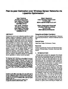
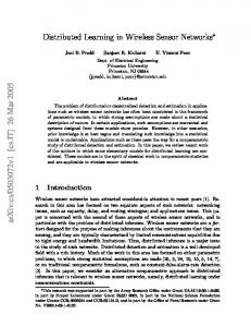
In this section we report some numerical results with the purpose to compare our strategy with other solutions from the literature. In particular, we considered a solution, denoted Eav , where the new estimate is the average between previous estimates and the current input. We also consider a solution where the weights are computed based on the Laplacian matrix associated to the communication graph, which we denoted with Elap . The estimator proposed in this paper is denoted with Enew . Simulations were carried out for two networks, with N = 20 and N = 35 nodes randomly distributed on an environment of size N/2 × N/2. Pair √ of nodes communicate only if their distance is less than 2 N . The signal to track is shown in the first plot of Fig. 2. Simulations were carried out for four cases of packet losses: perfect connectivity, p = 0.9, p = 0.7, and p = 0.5. The noise variance was chosen to be σ 2 = 1.5, which corresponds to a high peak signal to noise ratio. Time series of the estimates for our solution Enew , the Average Estimator Eav and the Laplacian Elap are reported in Fig. 2 for the cases of N = 20 and p = 0.3. The good behavior of Enew can be clearly noticed. It can be show that it remains basically the same also for other scenarios of number of nodes and packet loss. In order to compare the different solutions, we consider the average of the mean square estimation error over all the nodes of the network, which we denote MSE. As performance index we consider µi =
MSE(Ei ) − MSE(Enew ) , MSE(Ei )
i ∈ {av, lap} .
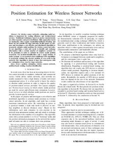
A summary of the results of the simulations is shown in Fig. 1, where each curve is referred to the pair estimatornetwork size. The performance improvement of our filter is evident in any situation of packet losses. Specifically, when N = 20, averaging over different q, there is an improvement of µN=20 av =52% with respect to the Average estimator and of about µN=20 lap =59% with respect to the Laplacian. In the case of N = 35, we obtain a µN=35 av =51% with respect to Average estimator and of about µN=35 = 62% with respect to the lap Laplacian. In Fig. 3 we show the value of γ(K(t)) for the simulation with N = 20 nodes and for different values of q.
γ(K(t)) for q = 0
Comparison between the three strategies for different network sizes
γ(K(t)) for q = 0.1
N=20 N=20
0.9
N=20
0.8
N=35 N=35
0.7
N=35
0.6
200
400
600
800
1000
0.5 0
200
400
t
600
800
1000
800
1000
t
γ(K(t)) for q = 0.3
γ(K(t)) for q = 0.5 1 0.9 0.8 0.7
0.05
0.1
0.15
0.2
0.25 q
0.3
0.35
0.4
0.45
0.6
0.5
200
400
600
800
1000
0.5 0
t
Fig. 1. Performance comparison among the different filtering strategies. The curves refer to the three estimators, Average, Laplacian and the one proposed in this paper for networks with N = 20 and N = 35.
200
400
600 t
Fig. 3. Value of γ(K(t)) as function of t for different values of q for the case N = 20.
Measurements 20 10 0
R EFERENCES 0
200
400
600
800
1000 1200 t Average Estimator
1400
1600
1800
2000
0
200
400
600
800
1400
1600
1800
2000
0
200
400
600
800
1400
1600
1800
2000
0
200
400
600
800
1400
1600
1800
2000
15 10 5
1000 1200 t Laplacian Estimator
15 10 5
1000 1200 t Proposed Estimator
15 10 5
1000 t
1200
Fig. 2. Signals representing the estimate and the measurements of d(t) for each of the 20 nodes in the network when p = 0.3.
As it can be clearly seen the maximum singular value is always below 1, thus confirming the validity of the local constraint in (6) adopted to the design of the filter coefficients. VIII. C ONCLUSIONS In this paper, we have presented a decentralized cooperative estimation algorithm for tracking a time-varying signal using a wireless sensor network. A mathematical framework is proposed to design a filter, which is supposed to run locally in each node of the network. As a relevant contribution, performance analysis has been carried out including time varying communication networks with Bernoulli models of the wireless channel. Theoretical analysis shows that the filter is stable, and the variance of the estimation error is bounded even in the presence of large packet losses probabilities. Numerical results illustrate the validity of our approach. ACKNOWLEDGMENT The authors thank Prof. M. Johannson, and Prof. B. Wahlberg for interesting and fruitful discussions.
[1] A. Savvides, W. L. Garber, R. L. Moses, and M. B. Srivastava, “An analysis of error inducing parameters in multihop sensor node localization,” IEEE Transaction on Mobile Computing, Vol. 4, No. 6, 2005. [2] A. Speranzon, C. Fischione, and K. H. Johansson, “Distributed and collaborative estimation over wireless sensor networks,” in In Proc. of IEEE CDC, 2006. [3] ——, “A distributed estimation algorithm for tracking over wireless sensor networks,” in IEEE ICC, 2007. [4] D. P. Bertsekas and J. N. Tsitsiklis, Parallel and Distributed Computation: Numerical Methods. Athena Scientific, 1997. [5] L. Xiao, S. Boyd, and S. Lall, “A scheme for robust distributed sensor fusion based on average consensus,” In Proc. of IEEE IPSN, 2005. [6] L. Xiao, S. Boyd, and S. J. Kim, “Distributed average consensus with least-mean-square deviation,” Submitted to Journal of Parallel and Distributed Computing, 2006. [7] L. Xiao and S. Boyd, “Fast linear iterations for distributed averaging,” System Control Letter, 2004. [8] R. Olfati-Saber and J. S. Shamma, “Consensus filters for sensor networks and distributed sensor fusion,” In Proc. of IEEE CDC, 2005. [9] G. L. St¨uber, Priciples of Mobile Communication. Kluwer Academic Publishers, 1996. [10] R. A. Horn and R. Mathias, “An analog of the Cauchy-Schwarz inequality for Hadamard products and unitarily invariant norms,” SIAM J. on Mat. Anal. and App., vol. 11, no. 4, pp. 481–498, 1990. [11] A. Speranzon, C. Fischione, and K. H. Johansson, “A distributed minimum variance estimator for wireless sensor networks,” School of Electrical Engineering, KTH, Sweden, Tech. Rep., 2007. [12] R. A. Horn and C. R. Johnson, Matrix Analysis. Cambridge University Press, 1985. [13] S. Boyd and L. Vandenberghe, Convex Optimization. Cambridge, UK: Cambridge University Press, 2004. [14] L. Ljung, System Identification: Theory for the User (2nd Edition). Prentice Hall PTR, 1998. [15] L. Ljung and B. Walhberg, “Asymptotic properties of the least-squares method for estimating transfer functions and disturbance spectra,” Adv. in App. Prob., vol. 24, no. 2, 1992. [16] G. H. Golub and U. Von Matt, “Tikhonov regularization for large scale problems,” Stanford SCCM, Stanford, Tech. Rep. 97-03, 1997. [17] M. T. Chao and W. E. Strawderman, “Negative moments of positive random variables,” Journal of the American Statistical Association, vol. 67, no. 388, 1972.