Adaptive Dynamic Programming.fm

---DRAFT--Adaptive Dynamic Programming J. Murray Department of Electrical Engineering State University of New York at Stony Brook Stony Brook, NY 11790 and C. Cox, G. Lendaris1, J. Neidhoefer, and R. Saeks Accurate Automation Corporation2 7001 Shallowford Rd. Chattanooga, TN 37421 February 1, 2001 Revised February 13, 2001, February 21, 2001, March 6, 2001

Abstract An Adaptive Dynamic Programming algorithm for nonlinear systems with unknown dynamics is developed. The algorithm is initialized with a positive definite cost functional / stabilizing control law pair (V0, k0) (coupled via the Hamilton Jacobi Bellman Equation). Given (Vi, ki), one runs the system using control law ki recording the state and control trajectories, with these trajectories used to define Vi+1 as the cost to take the initial state x0 to the final state using control law, ki, while ki+1 is taken to be the control law derived from Vi+1 via Hamilton Jacobi Bellman Equation. In this paper we show that this process is globally convergent with step-wise stability to the optimal cost functional / control law pair, (Vo, ko), for an (unknown) input affine system with an input quadratic performance measure (modulo the appropriate technical conditions). Furthermore, three specific implementations of the Adaptive Dynamic Programming algorithm are developed; for i) the linear case, ii) for the nonlinear case using a locally quadratic approximation to the cost functional, and iii) the nonlinear case using a (potentially global) radial basis function approximation of the cost functional; illustrated by applications to flight control.

1. INTRODUCTION Unlike the many soft computing applications where it suffices to achieve a “good approximation most of the time”, a control system must be stable all of the time. As such, if one desires to learn a 1. On Sabbatical Leave from Portland State University. 2. This research performed in part on NSF SBIR contracts DMI-9660604, DMI-9860370, and DMI9983287, NASA Ames SBIR Contracts NAS2-98016 and NAS2-20008, and NSF Grant ECS-9904378. Accurate Automation Corporation Proprietary - Nothing on this Page is Classified. Page 1

Adaptive Dynamic Programming

control law in real-time, a fusion of soft computing techniques to learn the appropriate control law with hard computing techniques to maintain the stability constraint and guarantee convergence is required. The objective of the present paper is to describe an Adaptive Dynamic Programming Algorithm which uses soft computing techniques to learn the optimal cost (or return) functional for a stabilizable nonlinear system with unknown dynamics and hard computing techniques to verify the stability and convergence of the algorithm. The present work has its roots in the approximate Dynamic Programming / adaptive critic concepts of [Barto, A., Sutton, R.S., C.W. Anderson, (1983)][Werbos, P.J. (1994)][Prokhorov, D. and L. Feldkamp. (1997)][Zaman, R., Prokhorov, D., and D. Wunsch. (1997)][Lendaris, G., Schultz, L., and T. Shannon, (2000)] in which soft computing techniques are used to approximate the solution of a dynamic programming algorithm without the explicit imposition of a stability or convergence constraint, and the authors’ stability criteria for these algorithms [Cox, C., Stepniewski S.W., Jorgensen C.C, and R. Saeks, (1999)][Saeks, R., and C. Cox, (1998)]. Alternatively, a number of authors have combined hard and soft computing techniques to develop tracking controllers. These include Lyapunov synthesis techniques using both neural [Sanner, R.M., and J.E. Slotine, (1991)][Wang, L.-X.,(1993)][Liu, G.P., Kadkivkamanthan, V., and S. A. Billings, (1999)][Cox, C., M. Lothers, R. Pap, and C. Thomas. (1992)][Saeks, R., and C. Cox (1997)] and fuzzy learning laws [Wang, L.-X.,(1993)][Wang, L.-X.,(1996)][Lingari, G., and M. Tomizuko, (1990)], sliding mode techniques [Wu, J.C., and T.S. Liu, (1996)], and input-output techniques [Ge, S.S., Hang, C.C., and T. Zhang, (1999)]. The centerpiece of Dynamic Programming is the Hamilton Jacobi Bellman (HJB) Equation [Bellman, R.E., (1957)][Bertsekas, D.P., (1987)][Luenberger, D.G., (1979)] which one solves for the optimal cost functional, Vo(x0, t0). This equation characterizes the cost to drive the initial state, x0, at time to to a prescribed final state using the optimal control. Given the optimal cost functional, one may then solve a second partial differential equation (derived from the HJB Equation) for the corresponding optimal control law, ko(x, to), yielding an optimal cost functional / optimal control law pair, (Vo, ko). Although direct solution of the Hamilton Jacobi Bellman Equation is computationally untenable (the so-called “curse of dimensionality”), the HJB Equation and the relationship between Vo and the corresponding control law, ko, derived therefrom, serves as the basis of the Adaptive Dynamic Programming Algorithm developed in the present paper. In this algorithm we start with an initial cost functional / control law pair, (V0, k0), where k0 is a stabilizing control law for the plant, and construct a sequence of cost functional / control law pairs, (Vi, ki), in real-time, which converge to the optimal cost functional / control law pair, (Vo, ko) as follows.

•

Given (Vi, ki); i = 0, 1, 2, … ; we run the system using control law ki from an array of initial conditions, x0, covering the entire state space (or that portion of the state space where one expects to operate the system);

•

recording the state, x i ( x 0, · ) , and control trajectories, u i ( x 0, · ) , for each initial condition.

Accurate Automation Corporation Proprietary - Nothing on this Page is Classified. Page 2


•

Given this data, we define Vi+1 to be the cost to take the initial state x0 at time t0, to the final state, using control law, ki, and

• •

take ki+1 to be the corresponding control law derived from Vi+1 via HJB Equation; iterating the process until it converges.

Indeed, in the following Section and in Appendix B it is shown that (with the appropriate technical assumptions) this process is:

• • •

globally convergent to the optimal cost functional, Vo, and the optimal control law, ko, and is stepwise stable; i.e., ki is a stabilizing controller at every iteration with Lyapunov function, Vi.

Since stability is an asymptotic property, technically it is sufficient that ki be stabilizing in the limit. In practice, however, if one is going to run the system for any length of time with control law, ki, it is necessary that ki be a stabilizing controller at each step of the iterative process. As such, for this class of adaptive control problems we “raise the bar”, requiring stepwise stability; i.e., stability at each iteration of the adaptive process, rather than simply requiring stability in the limit. Moreover, a-priori knowledge of the state dynamics matrix is not required to implement the algorithm, while the requirement that the input matrix be known (to compute ki+1 from Vi+1), can be circumvented by the pre-compensator technique described in Appendix A. As such the above described Adaptive Dynamic Programming Algorithm can be applied to plants with completely unknown dynamics. While one must eventually explore the entire state space (probably repeatedly) in any (truly) nonlinear control problem with unknown dynamics, in the above described Adaptive Dynamic Programming Algorithm one must explore the entire state space at each iteration of the algorithm (by running the system from an array of initial states which cover the entire state space). Unfortunately, this is not feasible and is tantamount to fully identifying the plant dynamics at each iteration of the algorithm. As such, Sections 3. - 5. of the present paper are devoted to the development of three approximate implementations of the Adaptive Dynamic Programming Algorithm which do not require global exploration of the state space at each iteration. These include:

•

the linear case, where one can evaluate ki+1 and Vi+1 from n local observations of the system state at each iteration;

•

an approximation of the nonlinear control law at each point of the state space, derived using a quadratic approximation of the cost functional at that point, requiring n(n+1)/2 local observations of the system state at each iteration; and



•

a nonlinear control law, derived at each iteration of the algorithm from a radial basis function approximation of the cost functional, which is updated locally at each iteration using data obtained along a single state trajectory.

2. ADAPTIVE DYNAMIC PROGRAMMING ALGORITHM In the formulation of the Adaptive Dynamic Programming Algorithm and Theorem, we use the following notation for the state and state trajectories associated with the plant. The variable “x” denotes a generic state while “x0” denotes an initial state, “t” denotes a generic time and “t0” denotes an initial time. We use the notation, x(x0, ·), for the state trajectory produced by the plant (with an appropriate control) starting at initial stare x0 (at some implied initial time), and the notation, u(x0, ·), for the corresponding control. Finally, the state reached by a state trajectory at time “t” is denoted by x = x(x0, t), while the value of the corresponding control at time “t” is denoted by u = u(x0, t). For the purposes of the present paper, we consider a stabilizable time-invariant input affine plant of the form x· = f ( x, u ) ≡ a ( x ) + b ( x )u; x ( t 0 ) = x 0

(1)

with input quadratic performance measure ∞

J =

ò l ( x ( ( x 0,

λ ) , u ( x 0 , λ ) ) ) dλ

t0

(2)

∞ T

≡ ò [ q ( x ( x 0, λ ) ) + u ( x 0, λ )r ( x ( x 0, λ ) )u ( x 0, λ ) ] dλ t0 ∞

Here a(x), b(x), q(x), and r(x) are C matrix valued functions of the state which satisfy: 1

a(0) = 0, producing a singularity at (x,u) = (0,0);

2

da ( 0 ) the eigenvalues of -------------- have negative real parts, i.e., the linearization of the uncontrolled dx plant at zero is exponentially stable;

3

q ( x ) > 0, x ≠ 0; q ( 0 ) = 0 ; 2

4

5

d q(0) > 0 , i.e., any non-zero state is penalized q(x) has a positive definite Hessian at x = 0, ---------------2 dx independently of the direction from which it approaches 0; and r(x) > 0 for all x.



The goal of the Adaptive Dynamic Programming Algorithm is to adaptively construct an optimal control, uo(x0, ·), which takes an arbitrary initial state, x0, at t0 to the singularity at (0,0), while minimizing the performance measure, J. Since the plant and performance measure are time invariant, the optimal cost functional and optimal control law are independent of the initial time, t0, which we may, without loss of o

o

o

o

generality, take to be 0; i.e. V ( x 0, t0 ) = V ( x 0 ) and k ( x, t 0 ) ≡ k ( x ) . Even though the optimal cost functional is defined in terms of the initial state, it is a generic function of the state, Vo(x), and is used in this form in the Hamilton Jacobi Bellman Equation and throughout the paper. Finally, o

o

we adopt the notation F ( x ) ≡ a ( x ) + b ( x )k ( x ) , for the optimal closed loop feedback system. Using this notation, the Hamilton Jacobi Bellman Equation then takes the form o

( x )- o o oT o dV ---------------F ( x ) = – l ( x, k ( x ) ) = – q ( x ) – k ( x )r ( x )k ( x ) dx

(3)

in the time-invariant case [Luenberger, D.G., (1979)]. Differentiating the HBJ Equation (3) with respect to uo = ko(x) now yields o

dV ( x )oT ---------------b ( x ) = – 2k ( x )r ( x ) dx

(4)

or equivalently o

o 1 –1 T dV ( x ) u = k ( x ) = – --- r ( x )b ( x ) ----------------dx 2

T

(5)

which is the desired relationship between the optimal control law and the optimal cost functional. Note, that an input quadratic performance measure is required to obtain the explicit form for ko in terms of Vo of Equation 5, though a similar implicit relationship can be derived in the general case. (See [Saeks, R., and C. Cox, (1998)] for a derivation of this result). Given the above preparation, we may now formulate the desired Adaptive Dynamic Programming Algorithm as follows. Adaptive Dynamic Programming Algorithm: 1

Initialize the algorithm with a stabilizing cost functional / control law pair (V0, k0), where V0(x) is a C

∞

function, V0 ( x ) > 0, x ≠ 0; V0 ( 0 ) = 0 , with a positive definite Hessian at x =

2

d V0 ( 0 ) dV 0 ( x ) 1 –1 ∞ T 0, ------------------> 0 ; and k0(x), is the C control law, u = k 0 ( x ) = – --- r ( x )b ( x ) ----------------2 2 dx dx

T

.



2

For i = 0, 1, 2, ... run the system with control law, ki, from an array of initial conditions, x0 at t0 = 0, recording the resultant state trajectories, xi(x0,·), and control inputs ui(x0,·) = ki(xi(x0,·)).

3

For i = 0, 1, 2, ... let ∞

V i + 1 ( x 0 ) ≡ ò l ( x i ( x 0, λ ), u ( u i ( x 0, λ ) ) ) dλ 0

and dVi + 1 ( x ) 1 –1 T u = k i + 1 ( x ) = – --- r ( x )b ( x ) ---------------------2 dx

T

where, as above, we have defined Vi+1 in terms of initial states but use it generically. 4

Go to 2.

Since the state dynamics matrix, a(x), does not appear in the above algorithm one can implement the algorithm for a system with unknown a(x). Moreover, one can circumvent the requirement that b(x) be known in Step 3, by augmenting the plant with a known pre-compensator at the cost of increasing its dimensionality, as shown in Appendix A. As such, the Adaptive Dynamic Programming Algorithm can be applied to plants with completely unknown dynamics. As indicated in the introduction, however, the requirement that one fully explore the state space at each iteration of the algorithm is tantamount to identifying the plant dynamics. As such, the applicability of the Adaptive Dynamic Programming Algorithm to plants with unknown dynamics is only meaningful in the context of the approximate implementations of Sections 3. 5., where only a local exploration of the state space is required. In the following we adopt the notation Fi for the closed loop system defined by the plant and control law, ki. dVi ( x ) 1 –1 T x· = F i ( x ) ≡ a ( x ) + b ( x )k i ( x ) = a ( x ) – --- b ( x )r ( x )b ( x ) --------------2 dx

T

(6)

To initialize the Adaptive Dynamic Programming Algorithm for a stable plant, one may take T

V 0 ( x ) = εx x and k0(x) = -εr-1(x)bT(x)x which will stabilize the plant for sufficiently small ε (though in practice we often take k0(x) = 0). Similarly, for a stabilizable plant, one can “pre2

d V0( 0) - > 0 and the stabilize” the plant with any desired stabilizing control law such that ------------------2 dx dF0 ( 0 ) - have negative real parts; and then initialize the Adaptive Dynamic eigenvalues of ---------------dx Accurate Automation Corporation Proprietary - Nothing on this Page is Classified. Page 6


Programming Algorithm with the above cost functional / control law pair. Moreover, since the state trajectory going through any point in state space is unique, and the plant and controller are time-invariant, one can treat every point on a given state trajectory as a new initial state when evaluating Vi+1(x0), by shifting the time scale analytically without rerunning the system. The Adaptive Dynamic Programming Algorithm is characterized by the following Theorem. Adaptive Dynamic Programming Theorem: Let the sequence of cost functional / control law pairs (Vi, ki); i = 0, 1, 2, ... ; be defined by, and satisfy the conditions of the Adaptive Dynamic Programming Algorithm. Then, i) Vi + 1 ( x ) and ki+1(x) exist, where Vi+1(x) and ki+1(x) are C

∞

functions with

2

d Vi + 1 ( 0) - > 0 ; i = 0, 1, 2, ... . V i + 1 ( x ) > 0, x ≠ 0; Vi + 1 ( 0 ) = 0; ------------------------2 dx ii) The control law, ki+1, stabilizes the plant (with Lyapunov function Vi+1(x)) for dFi + 1 ( 0 ) - have negative real parts. all i = 0, 1, 2, ... , and that the eigenvalues of ---------------------dx iii) The sequence of cost functional / control law pairs, (Vi+1, ki+1), converge to the optimal cost functional / control law pair, (Vo, ko). Note that in ii), the existence of the Lyapunov function Vi+1(x) together with the eigenvalue dFi + 1 ( 0 ) - implies that the closed loop system, Fi+1(x), is exponentially stable condition on ---------------------dx [Halanay, A., and Rasvan, V., (1993)], rather than asymptotically stable, as implied by the existence of the Lyapunov function alone. In the following, we sketch the proof of the Adaptive Dynamic Programming Theorem, while the details of the proof appear in Appendix B. The proof includes 4 steps as follows. 1

Show

that

Vi + 1 ( x )

and

ki+1(x)

exist

and

are

C

∞

functions,

with

V i + 1 ( x ) > 0, x ≠ 0; Vi + 1 ( 0 ) = 0 ; i = 0, 1, 2, ... . ∞

The first step required to prove that V i + 1 ( x ) and ki+1(x) exist and are C functions, is to show that the state trajectories defined by the control law ki and their derivatives with respect to the initial condition are integrable. Since ki is a stabilizing control law the state trajectories xi(x0,·) are asymptotic to zero. Although this implies that they are bounded, it is not sufficient dFi ( 0 ) for integrability. In combination with the condition that the eigenvalues of ---------------- have negadx Accurate Automation Corporation Proprietary - Nothing on this Page is Classified. Page 7


tive real values, however, asymptotic stability implies exponential stability [Halanay, A., and Rasvan, V., (1993)], which is sufficient to guarantee integrability. Intuitively, asymptotic stability guarantees that the state trajectories will eventually converge to a neighborhood of zero where the closed loop system defined by Fi may be approximated by the linear system defined dF i ( 0 ) dFi ( 0 ) - , which is exponentially stable since the eigenvalues of --------------- have negative real by --------------dx dx values. See [Halanay, A., and Rasvan, V., (1993)] for the details of this theorem. Similarly, one can show that the derivatives of the state trajectories with respect to the initial n ∂ x i ( x 0, . ) condition, ----------------------, are exponentially stable by showing that they also satisfy a differential n ∂x 0 dFi ( 0 ) equation which may be approximated in the limit by the linear system defined by ---------------- . dx Moreover, since the state trajectories and their derivatives with respect to the initial condition are exponentially stable, it follows from the defining properties for the plant and performance measure, that l ( x i ( x 0, . ), u ( u i ( x 0, . ) ) ) and its derivatives with respect to the initial condition are also exponentially convergent to zero. As such, l ( x i ( x 0, . ), u ( u i ( x 0, . ) ) ) and its derivatives with respect to the initial condition are ∞

∞

integrable, while they are C functions, since Fi is a C function [Dieudonne, J., (1960)]. As such, ∞

Vi + 1 ( x 0 ) ≡ ò l ( x i ( x 0, λ ), u ( ui ( x 0, λ ) ) ) dλ

(7)

0

and dV i + 1 ( x ) 1 –1 T k i + 1 ( x ) = – --- r ( x )b ( x ) ----------------------2 dx

T

(8)

∞

exist and are C functions. 2

Show that the Iterative Hamilton Jacobi Bellman Equation dVi + 1 ( x ) ---------------------- F i ( x ) = – l ( x, k i ( x ) ) dx 2

d Vi + 1 ( 0 ) - > 0 ; i = 0, 1, 2, ... . is satisfied, and that ------------------------2 dx



The iterative HJB Equation, which may be used as an alternative to Equation 7 for implementing the Adaptive Dynamic Programming algorithm, is derived by computing dVi + 1 ( x i ( x 0, t ) ) --------------------------------------- via the chain rule to obtain the left side of the Iterative HJB Equation, and dt by directly differentiating Equation 7 to obtain the right side of the equation. Then if one takes the second derivative of both sides of the resultant equation, evaluates it at x = 0, and drops dV i + 1 ( 0 ) those terms which contain ----------------------- or Fi ( 0 ) , both of which are zero; one obtains the Linear dx Lyapunov Equation 2

2

dFi ( 0 ) T d Vi + 1 ( 0 ) d V i + 1 ( 0 ) dFi ( 0 ) ---------------- -------------------------- + -------------------------- ---------------2 2 dx dx dx dx 2

2

d Vi + 1 ( 0 ) Vi + 1 ( 0 ) d q ( 0 -) 1--- d------------------------- ( b ( x )r –1 ( x )b T ( x ) ) ------------------------= – ---------------+ 2 2 2 2 dx dx dx 2

(9)

T

dF i ( 0 ) Now, since the eigenvalues of ---------------- have negative real parts, while the right side of Equadx tion 9 is a negative definite symmetric matrix, the unique symmetric solution of the Linear 2

d Vi + 1 ( 0 ) - > 0 , as Lyapunov Equation 9 is positive definite [Barnett, S., (1971)] and, as such, ------------------------2 dx required. 3

Show that Vi+1(x) is a Lyapunov Function for the Closed Loop System, Fi+1, and that the dF i + 1 ( 0 ) - have negative real parts; i = 0, 1, 2, ... . eigenvalues of ---------------------dx dV i + 1 ( x i + 1 ( x 0, t ) ) This is achieved by directly computing ---------------------------------------------- , i.e., the derivative of Vi+1(x) dt along the trajectories of the closed loop system, Fi+1, with the aid of the chain rule and the Iterative HJB equation, implying that ki+1 is a stabilizing controller for the plant for all i = 0, 1, 2, ... . dF i + 1 ( 0 ) - have negative real parts, we use an argument simiTo show that the eigenvalues of ---------------------dx lar to that used in 2, taking the second derivative of the expression derived for dVi + 1 ( x ) dVi + 1 ( x i + 1 ( x 0, t ) ) ----------------------- Fi + 1 ( x ) = ---------------------------------------------derived above. dx dt



4

Show that the sequence of cost functional / control law pairs, (Vi+1, ki+1) is convergent. This is achieved by showing that the derivative of Vi+1(x)-Vi(x) is positive along the trajectod [ V i + 1 ( x i ( x 0, t ) ) – Vi ( x i ( x 0, t ) ) ] ries of Fi, -------------------------------------------------------------------------------- > 0 , for i = 1, 2, 3, ... . Moreover, since Fi is dt asymptotically stable, its state trajectories, xi(x0,t), converge to zero, and hence so does d [ Vi + 1 ( x i ( x 0, t ) ) – Vi ( x i ( x 0, t ) ) ] Vi+1(xi(x0,t))-Vi(xi(x0,t)). Since -------------------------------------------------------------------------------- > 0 along these trajectories, dt however, this implies that Vi+1(xi(x0,t))-Vi(xi(x0,t)) < 0 on the trajectories of Fi; i = 1, 2, 3, ... . Since every point in the state space lies along some trajectory of Fi this implies that Vi+1(x)Vi(x) < 0, or equivalently, Vi+1(x) < Vi(x) for all x; i = 1, 2, 3, ... . As such, Vi+1 is a decreasing sequence of positive functions; i = 1, 2, 3, ... ; and is therefore convergent (as is the sequence Vi+1; i = 0, 1, 2, ... ; since the behavior of the first entry of a sequence does not affect its convergence). Note, the requirement that i ≥ 1 in this step of the proof is a “physical fact” and not just a “mathematical anomaly”, as indicated by the examples of Sections 3.-5., where the “cost-togo” from a given state typically jumps from its initial value for i = 0 to a large value, and then monotonically decreases to the optimal cost as one runs the algorithm for i = 1, 2, 3, ... .

3. THE LINEAR CASE The purpose of this section is to develop an implementation of the Adaptive Dynamic Programming algorithm for the linear case, where local exploration of the state space at each iteration of the algorithm is sufficient, yielding a computationally tractable algorithm. For this purpose we consider a linear time-invariant plant x· = Ax + Bu; x ( t0 ) = x 0

(10)

with the quadratic performance measure ∞

J =

ò [x

T

T

( x 0, λ )Qx ( x 0, λ ) + u ( x 0, λ )Ru ( x 0, λ ) ] dλ

(11)

t0

Here Q is a positive matrix, while R is positive definite. For this case Vo(x) = xTPox is a quadratic o

form,

where o

Po

is

a

positive

definite

matrix.

As

such,

dV T o -------( x ) = 2x P dx

and

–1 T o

u = K x = –R B P x . To implement the Adaptive Dynamic Programming Algorithm in the linear case, we initialize the –1 T

algorithm with a quadratic cost functional, V0(x) = xTP0x and K 0 = – R B P0 . Now, assuming



T

Vi ( x ) = x P i x

that

is

quadratic

–1 T

and

Ki = –R B P i ,

then

–1 T

F i ( x ) = [ A – BK i ]x = [ A – BR B Pi ]x ≡ Fi x ; where by abuse of notation we have used the symbol, Fi, for both the closed loop system and the matrix which represents it. As such, the state trajectories for the plant with control law Ki can be expressed in the exponential form Ft

Ft

x i ( x 0, t ) = e i x o , while the corresponding control is u i ( x 0, t ) = K i e i x o . As such, V i + 1 ( x0 ) =

T

ò

T

[ x i ( x 0, λ )Qx i ( x 0, λ ) + u i ( x 0, λ )Ru i ( x 0, λ ) ] dλ

0 ∞

=

ò

T Fi λ T

x0 e

Qe

Fi λ

T Fi λ T

xo + x0 e

Fλ T K i QK i e i x o

∞

dλ = x 0

0

T

òe

T

Fi t

T

[ Q + K i RK i ]e

Fi λ

dλ x o

(12)

0 ∞

= x0

T

òe

T

Fi t

–1 T

[ Q + P i BR B Pi ]e

Fi λ

T

dλ x o ≡ x 0 Pi + 1 x o

Now, since Fi is asymptotically stable the integral of Equation 12 exists, confirming that Vi+1(x) = xTPi+1x is also quadratic. Moreover, the integral defining Pi+1 is the “well known” integral form of the solution of the Linear Lyapunov Equation [Barnett, S., (1971)] T

–1 T

Pi + 1 Fi + Fi P i + 1 = – [ Q + P i BR B Pi ]

(13)

As such, in the linear case, rather directly evaluating the integral of Equation 12 one can iteratively solve for Pi+1 in terms of Pi by solving the Linear Lyapunov Equation (13). Note, that as an alternative to the above derivation one can obtain Equation 13 by expressing

dVi + 1 --------------- ( x ) dx

dVi + 1 T –1 T and Ki+1 in the form --------------- ( x ) = 2x Pi + 1 and K i + 1 = – R B P i + 1 , and substituting these dx expressions into the Iterative HJB Equation. –1 T

Although the A matrix for the plant is implicit in Fi ( = [ A – BR B P i ] ) , one can estimate Fi directly from measured data without a priori knowledge of A. To this end, one runs the system using control law Ki over some desired time interval, and observes the state at n (the dimension of the state space) or more points, xj; j = 1, 2, ... n; while (numerically) estimating the time derivative of the state at the same set of points; x· ; j = 1, 2, ... n. Now, since F is the closed loop j

i

system matrix for the plant with control law Ki, x· j = Fi x j ; j = 1, 2, … ; or equivalently · X i = F i Xi where X i = x 1 x 2 … x n . Assuming that the points where one observes the state are linearly independent, one can then solve for Fi from the observations via the equality Accurate Automation Corporation Proprietary - Nothing on this Page is Classified. Page 11


· –1 F i = X i Xi , yielding the alternative representation of the Linear Lyapunov equation · –1 · –1 T –1 T Pi + 1 [ X i Xi ] + [ X i Xi ] P i + 1 = – [ Q + Pi BR B Pi ]

(14)

which can be solved for Pi+1 in terms of Pi without a-priori knowledge of A. Moreover, one can circumvent the requirement that B be known via the pre-compensation technique of Appendix A. As such, Equation 14 can be used to implement the Adaptive Dynamic Programming Algorithm –1 without a-priori knowledge of the plant. Moreover, since F = X· X is asymptotically stable, i

i i

Equation 14 always admits a well defined positive definite solution, Pi+1, while there are numerous numerical solution techniques for solving this class of Linear Lyapunov Equations [Barnett, S., (1971)]. Moreover, unlike the full nonlinear algorithm, this implementation of the Adaptive Dynamic Programming Algorithm requires only local information at each iteration. Finally, if one implements the above algorithm off-line to construct the optimal controller for a · –1 system with known dynamics, using Fi at each iteration in lieu of Xi Xi , then the algorithm reduces to the Newton-Raphson iteration for solving the matrix Riccati Equation [Holley, W.E., and S.Y. Wei, (1979)][Kwakernaak, H., and R. Sivan, (1972)]. As an alternative to the above Linear Lyapunov Equation implementation, one can formulae an alternative implementation of linear Adaptive Dynamic Programming Algorithm using local information along a single state trajectory, xi(x0,·), and the corresponding control, u i ( x 0, · ) = K i x i ( x 0, · ) , starting at initial state x0 and converging to the singularity at (0,0). Indeed, for this trajectory one may evaluate Vi+1(x0) via ∞

Vi + 1 ( x0 ) =

ò [ xi

T

T

T

( x 0, λ )Qx i ( x 0, λ ) + u i ( x 0, λ )Rui ( x 0, λ ) ] dλ = x 0 Pi + 1 x 0

(15)

0

since the plant and control law are time-invariant. More generally, for any initial state, xj = xi(x0, tj), along this trajectory ∞

Vi + 1 ( xj ) =

ò [ xi

T

T

T

( x 0, λ )Qx i ( x 0, λ ) + u i ( x 0, λ )Ru i ( x 0, λ ) ] dλ = x 0 Pi + 1 x 0

(16)

tj

Now, since the positive definite matrix Pi+1 has only q = n(n+1)/2 independent parameters, one can select q (or more) initial states along this trajectory; xj; j = 1, 2, ..., q; and solve the set of simultaneous equations T

x j P i + 1 x j = V i + 1 ( x j ); j = 1, 2, …, q

(17)



for

Pi+1.

Equivalently,

applying

the

matrix

Kronecker

product

formula,

T

vec ( ABC ) = [ C ⊗ A ]vec ( B ) where the “vec” operator maps a matrix into a vector by stacking its columns on top of one another, one may transform Equation 17 into a q x n2 matrix equation T

T

T x2

T x2

x1 ⊗ x1 ⊗

Vi + 1 ( x1 ) vec ( Pi + 1 ) =

: T

T

xq ⊗ xq

Vi + 1 ( x2 )

(18)

: Vi + 1 ( xq )

Now, let “vec+” be the operator that maps an n x n matrix, B, to a q = n(n+1)/2 vector, vec+(B), by stacking the upper triangular part of its columns, b ij , i ≤ j , on top of one another. Now, if B is symmetric, vec+(B) fully characterizes B and, as such, one may define an n2 x q matrix, S, which maps vec+(B) to vec(B) for any symmetric matrix, B. As such, one may express Equation 18 in the form of a q x q matrix equation in the unknown vec+(Pi+1), æ ç ç ç ç ç ç è

T

T

T

T

x1 ⊗ x1 x2 ⊗ x2 : T xq

T

⊗ xq

ö ÷ ÷ + S÷÷ vec ( P i + 1 ) ÷ ÷ ø

V i + 1 ( x1 ) =

V i + 1 ( x2 )

(19)

: V i + 1 ( xq )

As such, assuming that the points where one observes the state are chosen to guarantee that Equation 19 has a unique solution, one can solve Equation 19 for a unique symmetric Pi+1. Moreover, since the general theory implies that Equation 19 has a positive definite solution, the unique symmetric solution of Equation 19 must, in fact, be positive definite. As such, one can implement the Adaptive Dynamic Programming Algorithm for a linear system by solving Equation 19 for Pi+1, instead of Equation 14. Although both Equations 14 and 19 require that one solve a linear equation in q = n(n+1)/2 unknowns, the derivatives of the state are not required by the Kronecker product formulation of Equation 19, while the Vi+1(xj) are computed by integrating along the entire state trajectory, thereby filtering any measurement noise. On the other hand, the Linear Lyapunov formulation of Equation 14 requires that one observe the state at only n points per iteration, and allows one to adapt the control multiple times along a given state trajectory. In both implementations one must assume that the xjs are chosen to guarantee that the appropriate matrix will be invertible. Although this is generically the case, this assumption may fail when one reaches the “tail” of the state trajectory. As such, in our implementation of the algorithm, we dither the state in the “tail” of a trajectory, and cease to update the control law when the state is near the singularity at (0,0).



To illustrate the implementation of the Adaptive Dynamic Programming Algorithm in the linear case, we developed an autolander for the NASA X-43 (or HyperX) [Singh, S.N., Yim, W., and W.R. Wells, (1995)]. The X-43, shown in Figure 1a, is an experimental testbed for an advanced a)

b)

Figure 1: a) NASA X-43 (HyperX) and b) its Glide Path scramjet engine operating in the Mach 7-10 range. In its present configuration, the X-43 is an expendable test vehicle, which will be launched from a Pegasus missile, perform a flight test program using its scramjet engine, after which it will crash into the ocean. The purpose of the simulation described here was to evaluate the feasibility of landing a follow-on series of X-43s. To this end, we developed an autolander for the X-43 designed to follow the glide path illustrated in Figure 1b, using the Adaptive Dynamic Programming Algorithm, and simulated its performance using a 6 degree-of-freedom linearized model of the X-43. This model has eleven states indicated in Table 1 and four inputs indicated in Table 2. To stress the adaptive controller, the simulation used an extremely steep glide path angle. Indeed, so steep that the drag of the aircraft was initially insufficient to cause the aircraft to fall fast enough, requiring negative thrust. Of course, in practice one would never use such a steep glide slope, alleviating the requirement for thrust reversers in the aircraft. To illustrate the adaptivity of the controller, no a-priori knowledge of either the A or B matrices for the X-43 model was provided to the controller. Table 1: States of Linearized 6 DoF X-43 Model State

Symbol

Units

Trim Value

Initial Error

roll rate

p

rad/s

0.0

0.0850

yaw rate

r

rad/s

0.0

0.0850

pitch rate

q

rad/s

0.0

0.0850

roll

phi

rad

0.0

0.0850

yaw

psi

rad

-0.0778

0.0850

pitch

theta

rad

0.0

0.0850

vertical component of airspeed

w

ft/s (positive in down direction)

96.1442

-20.0000

forward component of airspeed

u

ft/s

0.0

-20.0000

side component of airspeed

v

ft/s

30.6225

-20.0000



Table 1: States of Linearized 6 DoF X-43 Model side tracking error (side deviation from desired glide-path)

ft

0.0850

altitude tracking error (vertical deviation from desired glide-path)

ft

0.0850

Table 2: Inputs (symbol, units) of Linearized 6 DoF X-43 Model control

symbol

units

trim value

elevator deflection

de

deg

-15.86

rudder deflection

dr

deg

-0.0

control

symbol

units

aileron deflection

da

deg

thrust

dt

poun ds

trim value 0.0 10.728

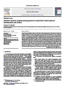
A “trim routine” is used to calculate the steady state settings of the aircraft control surfaces required to achieve the desired flight conditions, with the state variables and controlled inputs for the flight control system taken to be the deviations from the trim point. In the present example the trim control was calculated to maintain the aircraft on the specified glide slope. The performance of the X-43 autolander is summarized in Figure 2 where the altitude and lateral errors from the

Figure 2: X-43 Autolander Altitude Error, Lateral Error, and Sink Rate glide path and the vertical component of the aircraft velocity (sink rate) along the glide path are plotted. After correcting for the initial deviation from trim, the autolander brings the aircraft to, and maintains it on, the glide path. The control values employed by the autolander to achieve this level of performance are shown in Figure 3a, all of which are well within the dynamic range of the X-43’s controls, while the remaining states of the aircraft during landing are shown in Figures 3b, 3c, and 3d. To evaluate the adaption rate of the autolander, the “cost-to-go” from the initial state is plotted as a function of time as the controller adapts in Figure 4. As expected, the cost-to-go jumps from the Accurate Automation Corporation Proprietary - Nothing on this Page is Classified. Page 15


a)

b)

c)

d)

Figure 3: a) Aircraft Controls (de, da, dr, and T); b) Orientation Rates (p, q, and r); c) Orientation Angles (phi, theta, and psi); and Airspeed Components (u, v, and w).

Figure 4: Cost-to-Go from Initial State as a Function of Time low initial value associated with the initial guess, Po, to a relatively high value, and then decays monotonically to the optimal value as the controller adapts. Although the theory predicts that the cost-to-go jump should occur in a single iteration, a filter was used to smooth the adaptive process Accurate Automation Corporation Proprietary - Nothing on this Page is Classified. Page 16


in our implementation, which spreads the initial cost-to-go jump over several iterations

4. QUADRATIC APPROXIMATION OF THE COST FUNCTIONAL The purpose of this section is to develop an approximate implementation of the Adaptive Dynamic Programming Algorithm in which the actual cost functional is approximated by a ∞

quadratic at each point in state space. To this end, we let a(x), b(x), q(x), and r(x) be C functions dV i T as defined in Section 2., and we let Vi(x) = xTPix in which case -------- ( x ) = 2x Pi and dx –1

T

k i ( x ) = – r ( x )b ( x )Pi + 1 x are also C Iterative HJB Equation we obtain T

∞

functions. Substituting these expression into the

T

T

–1

x Pi + 1 x· = – q ( x ) – x P i b ( x )r ( x )b ( x )Pi x

(20)

Following the model developed for the Kronecker Product formulation of the linear algorithm in Section 3., we observe the state at q = n(n+1)/2 points; xj; j = 1, 2, ... , q; and solve the set of simultaneous equations T

T

T

–1

x j Pi + 1 x· j = – q ( x j ) – x j Pi b ( x j )r ( x j )b ( x j )Pi x j ; j = 1, 2…, q

(21)

or, equivalently in matrix form T T x· 1 ⊗ x 1

T

–1

T

– q ( x 1 ) – x 1 Pi b ( x1 )r ( x 1 )b ( x 1 )Pi x 1

T T T x· 2 ⊗ x 2 vec ( P ) = – q ( x 2 ) – x 2T Pi b ( x2 )r –1 ( x 2 )b ( x 2 )Pi x 2 i+1 : : T T T T –1 x· q ⊗ x q – q ( x q ) – x 2 Pi b ( xq )r ( x q )b ( x q )Pi x q

(22)

Unlike the linear case, however, where one could reduce the number of degrees of freedom of Pi+1 to q by requiring it to be hermitian, with positivity following from the fact that a positive definite solution of Equation 19 is known to exist, in the nonlinear case one cannot guarantee that a hermitian solution to Equation 22 will be positive definite. As such, we reduce the number of degrees of freedom of Pi+1 to q by expressing it as the product of an upper triangular matrix with T

positive diagonal entries, Ui+1, and its transpose, Pi + 1 = U i + 1 U i + 1 , forcing Pi+1 to be positive definite hermitian. Substituting this expression into Equation 22 we then solve the quadratic equation



T

T

–1

– q ( x1 ) – x 1 Pi b ( x 1 )r ( x 1 )b ( x 1 )Pi x 1

T T x· 1 ⊗ x 1

T T T x· 2 ⊗ x 2 vec ( U T U ) = – q ( x2 ) – x 2 T Pi b ( x 2 )r –1 ( x 2 )b ( x 2 )Pi x 2 i+1 i+1 : : T T x· q ⊗ x q

T

(23)

T

–1

– q ( xq ) – x q Pi b ( x q )r ( x q )b ( x q )Pi x q T

T

for Ui+1, yielding an approximation of the actual cost functional in the form x U i + 1 U i + 1 x . To circumvent the differentiation of the observed state trajectory, one can formulate an alternative implementation of the above algorithm using observations obtained along a state trajectory, x ( x , . ) , starting at initial state x0 and converging to the singularity at (0,0). As before, we i

0

approximate Vi(x) by a quadratic, xTPix, but work with the integral expression for Vi+1(x) rather than the Iterative HJB equation, obtaining the set of equations ∞

V i + 1 ( xj ) =

T

T

–1

ò [ q ( x i ( x 0, λ ) ) + x i ( x 0, λ )P i b ( x i ( x 0, λ ) )r ( x i ( x 0, λ ) )b ( x i ( x 0, λ ) )P i x i ( x 0, λ ) ] dλ (24) t j

T

= x j P i + 1 x j ; j = 1, 2, …, q for a sequence of initial states xj = xi(x0, tj); j = 1, 2, ... , q; along xi(x0, ·). Converting Equation 24 to Kronecker Product form now yields the q x n2 matrix equation T

T

T x2

T x2

x1 ⊗ x1 ⊗

Vi + 1 ( x1 ) vec ( Pi + 1 ) =

: T

T

xq ⊗ xq

Vi + 1 ( x2 )

(25)

: Vi + 1 ( xq )

T

or equivalently, letting P i + 1 = U i + 1 U i + 1 T

T

x1 ⊗ x1

Vi + 1 ( x1 )

T T x 2 ⊗ x 2 vec ( U T U ) = Vi + 1 ( x 2 ) i+1 i+1 : : T T Vi + 1 ( xq ) xq ⊗ xq

(26)

which may be solved for Ui+1, yielding an approximation of the actual cost functional in the form Accurate Automation Corporation Proprietary - Nothing on this Page is Classified. Page 18


T

T

x Ui + 1 Ui + 1 x . Although both Equations 22 and 26 require that one solve a quadratic equation in q = n(n+1)/2 unknowns, the derivatives of the state are not required by the formulation of Equation 26, while the Vi+1(xj) are computed by integrating along the entire state trajectory, xi(x0,·), from x0 to the singularity at (0,0) thereby filtering out “most” of the measurement noise. On the other hand, the formulation of Equation 22 allows one to adapt the control multiple times along a given state trajectory. In both implementations one must assume that the xjs are chosen to guarantee that the appropriate matrix will be invertible. As in the linear case, this assumption may fail when one reaches the “tail” of the state trajectory. To evaluate the performance of the Adaptive Dynamic Programming Algorithm of Equation 22, we selected the system illustrated in Figure 5. in which a unit mass (m = 1) is constrained to

v v = u2 m=1 c = .001

fV fH

g

u

Figure 5: Mass Constrained to a Parabolic Track follow a parabolic track (u = v2) under the influence of horizontal (fH) and vertical (fV) forces, gravity (g), and a small amount of viscous damping (c = 0.001). This 2nd order system, though somewhat academic, is highly nonlinear yet sufficiently well understood to allow us to evaluate the performance of the adaptive controller. Taking the state variables to be x2 = u and x 1 = x· 2 , this system has the input affine state model · x1 x2

2

2x 2 – 4x 1 x 2 – 2gx 2 – cx 1 1 -------------------------- -------------------------- fV ------------------------------------ ----------2 2 2 = + m m ( 1 + 4x ) m ( 1 + 4x ) 1 + 4x 2 2 2 fh 0 0 x1 0

(27)

Moreover, it is stable with a Lyapunov function taken to be the total (kinetic + potential) energy 2 2 2 m E = ---- ( 1 + 4x 2 )x 1 + mgx 2 2

(28)



while the derivative of E along the trajectories of the system takes the form 2 2 E· = – c ( 1 + 4x 2 )x 1

(29)

To evaluate the performance of the Adaptive Dynamic Programming Algorithm without a-priori knowledge of either a(x) or b(x), a 1st order pre-compensator was used (increasing the order of the system to 3 as per Appendix A). The state response of the system starting from initial state x0 = [1,2]T at t0 = 0 without control is shown in Figure 6a while the response of the controlled system a)

b)

Figure 6: a). Uncontrolled and b). Controlled Response of Parabolically Constrained Mass is shown in Figure 6b. Here, the controlled response converges to the singularity at (0,0) in less than 3 seconds with a reasonably smooth response, while the minimally damped uncontrolled system oscillates for several minutes before settling down.

5. RADIAL BASIS APPROXIMATION OF THE COST FUNCTIONAL Unlike the nonlinear implementation of the Adaptive Dynamic Programming algorithm of Section 4., where one approximates Vi+1(x) locally by a quadratic function of the state, the purpose of this section is to develop an implementation of the algorithm in which Vi+1(x) is approximated nonparametrically by a linear combination of radial basis functions. Since radial basis functions are “local approximators,” however, one can update the approximation locally in a neighborhood of each trajectory, xi(x0,·), without waiting to explore the entire state space. As such, an approximation of Vi+1(x), updated on the basis of a local exploration of the state space at each iteration, which is “potentially” globally convergent is obtained. To demonstrate the radial basis function implementation of the Adaptive Dynamic Programming algorithm we chose a 4th order longitudinal model of the LoFLYTE® UAV (Unmanned Autonomous Vehicle) with a nonlinear pitching moment coefficient, illustrated in 7. The states of the model are indicated in Table 3, with the zero point in the state space shifted to correspond to a



Figure 7: LoFLYTE® UAV at Edwards AFB selected trim point for the aircraft. The input for this model was the elevator deflection, with δ e = 0 in the model corresponding to a downward elevator deflection of -2.784o. Table 3: States of Nonlinear Longitudinal LoFLYTE® Model State

Symbol

Units

Min

Trim Point

Max

q

rad/s

-0.3491

0.0000

0.3491

theta

rad

-0.6850

-0.3359

0.0132

vertical component of airspeed

w

ft/s (positive in down direction)

-4.116

16.12

36.12

forward component of airspeed

u

ft/s

95.97

115.97

135.97

pitch rate pitch

For our radial basis function implementation of the Adaptive Dynamic Programming algorithm, each axis of the state space is covered by 21 radial-basis-functions, from a predetermined minimum to a predetermined maximum value indicated in Table 3. As such, that part of state space where the UAV operates is covered by 21x21x21x21=194,481 radial-basis-functions. Given the local nature of the radial basis functions, however, at any point in the state space Vi+1(x) is computed by summing the values a 5x5x5x5=625 block of radial basis functions in a neighborhood of x, corresponding to a 4-cube in state space centered at x with ∆u = +/-4.76 ft/s, ∆w = +/-4.76 ft/s, ∆q = +/-0.083 rad/s, and ∆θ = +/-0.083 rad. The following figures illustrate the performance of the radial basis function implementation of the Adaptive Dynamic Programming algorithm, learning an “optimal” control strategy from a given initial point in the state space, using the quadratic performance measure J =

∞ T ò 0 [ x Qx

T

+ u Ru ] dλ with

Q = diag [ .0015, .0015, .0015, .0015 ] and R = [.005]. The

algorithm was initiated on the 0th iteration with k0(x)=0. After the state converged to the trim point, the iteration count was incriminated, a radial basis function approximation of Vi+1(x) was computed, the new control law, ki+1(x), was constructed, and the system was restarted at the same Accurate Automation Corporation Proprietary - Nothing on this Page is Classified. Page 21


initial state. In these simulations, the aircraft state was updated 100 times per second while the elevator deflection angle was updated 10 times per second. The performance of the radial basis function implementation of the Adaptive Dynamic Programming algorithm is illustrated in Figures 8 through 11, where we have plotted each of the key system variables on the 0th, 1st, 2nd, 3rd, 4th, 5th, iterations of the algorithm and the limiting value of these plots (at the 60th iteration). The state variables of the aircraft are plotted in Figure 8. For each state variable the initial (0th) a)

b) vertical com ponent of airspeed as function of tim e for each iteration

horizontal com ponent of airspeed as function of tim e for eac h iteration

horizontal com ponent of airspeed in feet per second

vertical com ponent of airspeed in feet per secopnd

17.4

17.2

limiting response 17

16.8

initial response

16.6

16.4

16.2

1st iteration

126

124

limiting response

122

120

1st iteration

118

initial response 116

16 0

1

2

3 tim e in seconds

4

5

0

6

c)

1

2

3 tim e in s ec onds

4

5

6

d) pitch rate as func tion of time for eac h iteration

pitch angle as func tion of time for each iteration -0.3

0.045

initial response

-0.31 -0.32

limiting response pitch angle in radians

pitch rate in radians per s econd

0.04 0.035 0.03 0.025 0.02

1st iteration

0.015

limiting response

-0.33 -0.34

1st iteration

-0.35 -0.36

0.01 -0.37

0.005

initial response

-0.38

0

-0.39

-0.005 0

1

2

3 time in seconds

4

5

6

0

1

2

3 time in seconds

4

5

6

Figure 8: Aircraft State Variables on the 0th, 1st, 2nd, 3rd, 4th, 5th and 60th Iteration: a) Vertical Velocity, b) Horizontal Velocity, c) Pitch Rate, and d) Pitch Angle. response (indicated by “x”s) is at one extreme (high for the vertical velocity, pitch, and pitch rate; and low for the horizontal velocity), with the response jumping to the opposite extreme on the 1st iteration (indicated by “o”s) and then converging toward the limiting value, with the adaption process effectively convergent after 10 iterations. The elevator deflection required to achieve these responses is show in Figure 9. Since k0(x)=0 the initial (0th) elevator deflection remains Accurate Automation Corporation Proprietary - Nothing on this Page is Classified. Page 22


elevator deflection as function of time for each iteration -2.4

1st iteration

-2.45

elevator deflec tion in degrees

-2.5 -2.55

limiting control

-2.6 -2.65 -2.7 -2.75 -2.8 -2.85 0

initial control 1

2

3 time in seconds

4

5

6

Figure 9: Elevator Deflection on the 0th, 1st, 2nd, 3rd, 4th, 5th and 60th Iteration constant at the trim point of -2.784o (indicated by “x”s). The elevator deflection then jumps to a high values on the 1st iteration (indicated by “o”s), and then converges toward the limiting value. All variables are well within a reasonable dynamic range for the LoFLYTE® UAV except for the initial drop of the aircraft (indicated by the initial positive spike in the vertical velocity curve of Figure 8a), due to the use of a “null” controller on the first iteration (which would not be the case for the actual aircraft where k0(x) would be selected on the basis of prior simulation). The performance of the Adaptive Dynamic Programming algorithm is illustrated in Figure 10 where the computed (Figure 10a) and radial basis function approximation (Figure 10b) of the optimal cost functional are plotted as a function of time along the state trajectory, on the 0th, 1st, a)

b) RBF output as function of time for each iteration 0.3

0.25

0.25

0.2

0.2

limiting approximation 0.15

RB F output

com puted V i

computed Vi as function of time for each iteration 0.3

1st iteration

limiting approximation 0.15

1st iteration 0.1

0.1

initial approximation

initial approximation 0.05

0.05

0

0 0

1

2

3 time in seconds

4

5

6

0

1

2

3 time in seconds

4

5

6

Figure 10: a) Computed and b) RBF Approximation of the Optimal cost functional on the 0th, 1st, 2nd, 3rd, 4th, 5th and 60th Iteration



2nd, 3rd, 4th, 5th, and 60th (limiting) iteration of the algorithm. In both cases, the initial estimate (indicated by “x”s) is low and converges upward to the limiting value, with the RBF approximation error decreasing in parallel with the adaption process. Finally, the cost-to-go based on the computed (“x”s) and radial basis function approximation (“o”s) of the optimal cost functional is plotted as a function of the iteration number in Figure 11. As predicted by the theory,

calculated Vi (-x-) & RBF output (-o-); same initial state used in each iteration 0.3

c alc ulated V i and RB F es tim ate of V i

0.28

0.26

0.24

0.22

0.2

0.18 0

10

20

30 iteration number

40

50

60

Figure 11: Cost-to-Go based on the Computed (“x”s) and RBF Approximation (“o”s) of the Optimal cost functional vs. Iteration Number the cost-to-go has an initial spike and then declines monotonically to the limiting value.

6. CONCLUSIONS Our goal in the preceding has been to provide the framework for a family of Asymptotic Dynamic Programming algorithms by developing the general, if not directly applicable, theory and the three implementations of Sections 3.-5. Indeed, several alternative implementations come to mind. First, by taking advantage of the intrinsic adaptivity of the algorithm, one could potentially use a linear adaptive controller on a nonlinear system, letting it adapt to a different linearization of the plant at each point in state space, effectively implementing an “adaptive gain scheduler.” dVi ( x ) - , not Vi(x), any approximation of the cost Secondly, since the control law is based on --------------dx functional should consider the gradient error as well as the direct approximation error. Therefore, in Section 5. one might replace the radial basis function approximation, which produces a “bumpy” Tchebychev-like approximation of Vi(x), with a “smoother” cubic spline approximation, or an alternative local approximator. Finally, by requiring the plant and performance measure ∞

matrices to be “real analytic” rather than C (and extending the proof of the theorem to guarantee that the matrices generated by the iterative process are also “real analytic”) one might consider the possibility of using analytic continuation to extrapolate local observations of the state space to the entire (or a larger region in the) state space, implementing the process with one of the modern symbolic mathematics codes.



7. REFERENCES Barnett, S., (1971). The Matrices of Control Theory, Van Norstrand Reinhold, New York. Barto, A., Sutton, R.S., C.W. Anderson, (1983). “Neuronlike Adaptive Elements That Can Solve Difficult Learning Problems,” IEEE Trans. on Systems, Men, and Cybernetics, Vol. 13, No.5, pp. 834-846. Bellman, R.E., (1957). Dynamic Programming, Princeton University Press, Princeton. Bertsekas, D.P., (1987). Dynamic Programming: Deterministic and Stochastic Models, PrenticeHall, Englewood Cliffs. Cox, C., M. Lothers, R. Pap, and C. Thomas. (1992). “A Neurocontroller for Robotics Applications.” In Proceedings of the Conference on Systems, Man, and Cybernetics, Chicago, pp. 712-716. Cox, C., Stepniewski S.W., Jorgensen C.C, and R. Saeks, (1999). “On the Design of a Neural Network Autolander”, Int. Jour. of Robust and Nonlinear Cont., Vol. 9, pp. 1071-1096. Devinatz, A., and Kaplan, J.L., (1972). “Asymptotic Estimates for Solutions of Linear Systems of Ordinary Differential Equations Having Multiple Characteristics Roots”, Indiana Univ. Math Journal, Vol. 22, p. 335. Dieudonne, J., (1960). Foundations of Mathematical Analysis, Academic Press, New York. Ge, S.S., Hang, C.C., and T. Zhang, (1999). “Adaptive Neural Network Control of Nonlinear Systems by Stable Output Feedback”, IEEE Trans. on Systems Man an Cybernetics: Part B, pp. 818-828. Halanay, A., and Rasvan, V., (1993). Applications of Liapunov Methods in Stability, Kluwer, Dordrecht. Holley, W.E., and S.Y. Wei, (1979). “An Inprovement in the MacFarlane-Potter Method for Solving the Algebraic Riccati Equation”, Proc. of the Joint Auto. Cont. Conf., pp. 921-923, Denver. Kwakernaak, H., and R. Sivan, (1972). Linear Optimal Control Systems, Wiley, New York. Lendaris, G., Schultz, L., and T. Shannon, (2000). “Adaptive Critic Design for Intelligent Steering and Speed Control of a 2-Axle Vehicle”, Proc. of the Inter. Joint Conf. on Neural Networks, Washington, (to appear). Lingari, G., and M. Tomizuko, (1990). “Stability of Fuzzy Linguistic Control Systems”, Proc. of the IEEE Decision and Control, Hawaii, pp. 2185-2190, Liu, G.P., Kadkivkamanthan, V., and S. A. Billings, (1999). “Variable Neural Network for Adaptive Control of Nonlinear Systems”, IEEE Trans. on Systems man and Cybernetics: Part C, Vol. 29, pp. 34-43. Luenberger, D.G., (1979). Introduction to Dynamic Systems: Theory, Models, and Applications, John Wiley and Sons, New York. Prokhorov, D. and L. Feldkamp. (1997). “Primitive Adaptive Critics,” In Proceedings of the 1997 International Conference on Neural Networks. Vol. IV, pp. 2263-2267. Saeks, R., and C. Cox (1997). “LoFLYTE®: a Neurocontrols Testbed”, 35th AIAA Aerospace Sciences Meeting, AIAA Paper 97-0085. Saeks, R., and C. Cox, (1998). “Adaptive Critic Control and Functional Link Networks”, Proc. of the 1998 IEEE Conf. on Systems, Man, and Cybernetics, San Diego, pp. 1652-1657. Sanner, R.M., and J.E. Slotine, (1991). “Gaussian Networks for Direct Adaptive Control”, Proc. of the Amer. Cont. Conf., pp. 2153-2159. Singh, S.N., Yim, W., and W.R. Wells, (1995). “Direct Adaptive and Neural Control of WingRock Motion of Slender Delta Wings”, Jour. of Guidance, Control and Dynamics, Vol. 18, pp. 25-30. Sitz, J., (1998). “HYPEER-X: Hypersonic Experimental Research Vehicle”, NASA Fact Sheet, FS-1994-11-030. Wang, L.-X.,(1993). “Stable Adaptive Fuzzy Control with Applications to Inverted Pendulum Tracking”, IEEE Trans. on Fuzzy Systems, Vol. 1, pp. 146-155. Wang, L.-X.,(1996). “Stable Adaptive Fuzzy Control of Nonlinear Systems”, IEEE Trans. on Systems Man an Cybernetics: Part B, pp. 677-691. Werbos, P.J. (1994). “Approximate Dynamic Programming For Real Time Control and Neural Modeling.” In Handbook of Intelligent Control. White and Sofge, Eds. Van Nostrand Reinhold. pp. 493-525. Wu, J.C., and T.S. Liu, (1996). “Fuzzy Control Stabilization with Applications to Motorcycle Control”, IEEE Trans. on Systems Man an Cybernetics: Part B, pp. 836-847. Accurate Automation Corporation Proprietary - Nothing on this Page is Classified. Page 25


Zaman, R., Prokhorov, D., and D. Wunsch. (1997 ). “Adaptive Critic Design in Learning to Play Game of Go.” In Proceedings of the 1997 International Conference on Neural Networks, Vol. I, pp. 1-4.

APPENDIX A. PRE-COMPENSATION PROCEDURE The purpose of this appendix is to derive the precompensation technique originally described in [Saeks, R., and C. Cox, (1998)], which embeds the b(x) matrix of an input affine plant into the a(x) matrix of the combined pre-compensator / plant model, thereby allowing one to apply the Adaptive Dynamic Programming techniques developed in the present paper for a plant with an unknown a(x) matrix, to a plant with both a(x) and b(x) unknown. This technique is illustrated in u· = α ( u ) + β ( u )v u ( 0 ) = uˆ

x· = a ( x ) + b ( x )u x ( 0 ) = xˆ

o v = k˜ ( x, u )

Figure 12: Control System with Pre-Compensator Figure 12, where, the pre-compensator is defined by any desired (controllable) input affine differential equation, u· = α ( u ) + β ( u )v , whose state vector is of the same dimension as the input vector for the given plant, with a singularity at (u=0, v=0). Now, the dynamics of the augmented plant, obtained by combining the pre-compensator with the original plant take the form · ·˜ x = x = a ( x ) + b ( x )u = a ( x ) + b ( x )u + 0 v α ( u ) + β ( u )v α( u) β( u) , u

(30)

= a˜ ( x, u ) + b˜ ( x, u )v = a˜ ( x˜ ) + b˜ ( x˜ )v which is also input affine, with the augmented state vector, x˜ = x u

T

and a singularity at

( x˜ =0,ν=0). Moreover, all of the dynamics of the original plant are now embedded in the a˜ ( x˜ ) matrix of the augmented plant with b˜ ( x˜ ) known (since the dynamics of the precompensator are specified by the system designer). Furthermore, we may define an augmented performance measure by J˜ = ∞

=

ò

0

∞

ò

0

[ ˜l ( x˜ ( x 0, λ ), v ( x 0, λ ) ) ] dλ ∞

(31)

[ l ( x ( x 0, λ ), u ( x 0, λ ) ) + l v ( v ( x0, λ ) ) ] dλ = J + ò [ lv ( v ( x 0, λ ) ) ] dλ t0



where lv ( v ( x 0, t ) ) ≥ 0 with equality if and only if ν=0. As such, one can apply the above described Adaptive Dynamic Programming Algorithm to a plant in which both a(x) and b(x) are unknown by applying the algorithm to the augmented system of Equation 30 with the augmented performance measure of Equation 31, yielding a control law o o of the form k˜ ( x˜ ) = k˜ ( x, u ) . This is, however, achieved at the cost of using a modified performance measure and increasing the dimension of the state space.

APPENDIX B.PROOF OF THE ADAPTIVE DYNAMIC PROGRAMMING THEOREM The proof of the Adaptive Dynamic Programming Theorem follows the 4 steps indicated in Section 2. 1

Show

that

Vi + 1 ( x )

and

ki+1(x)

exist

and

are

C

∞

functions

with

V i + 1 ( x ) > 0, x ≠ 0; Vi + 1 ( 0 ) = 0 ; i = 0, 1, 2, ... . By construction Vi + 1 ( x ) > 0, x ≠ 0; Vi + 1 ( 0 ) = 0 , while the existence and smoothness of ∞

k i + 1 ( x ) follows from that of Vi + 1 ( x ) since b(x) and r(x) are C functions and r-1(x) exists. As such, it suffices to show that V i + 1 ( x ) exists and is a C

∞

function. Since Vi + 1 ( x ) is

defined by the state trajectories generated by the ith control law, ki(x), we begin by characterizing the properties of the state trajectories xi(x0,·). In particular, since the control law and the ∞

∞

plant are defined by C functions, the state trajectories are also C functions of both x0 and t [Dieudonne, J., (1960)]. Furthermore, since ki(x) is a stabilizing controller and the eigenvalues dF i ( 0 ) of ---------------- have negative real parts, the state trajectories, xi(x0,·), converge to zero exponendx tially [Halanay, A., and Rasvan, V., (1993)]. In addition to showing that the state trajectories, xi(x0,·), are exponentially stable, we would also like to show that the partial derivatives of the state trajectories with respect to the initial n ∂ x i ( x 0, . ) ∂x i ( x 0, . ) --------------------- satcondition, ----------------------, are also exponentially stable. To this end we observe that n ∂x 0 ∂x 0 isfies the differential equation

∂x· i ( x 0, . ) ∂Fi ( x i ( x 0, . ) ) x i ( x 0, . ) ∂- ∂----------------------= --------------------- = -------------------------------∂x 0 ∂x 0 ∂x 0 ∂t dFi ( x i ( x 0, . ) ) = -------------------------------dx

∂x i ( x 0, . ) ∂x i ( x 0, 0 ) --------------------- ; ----------------------=1 ∂x 0 ∂x 0

(32)



Since xi(x0,·) is asymptotic to zero, Equation 32 reduces to the linear time-invariant differential equation ∂x i ( x 0, . ) dFi ( 0 ) ∂- ----------------------= ---------------∂t ∂x 0 dx

∂x i ( x 0, . ) ∂x i ( x 0 , 0 ) --------------------; ----------------------- = 1 ∂x 0 ∂x 0

(33)

∂x i ( x 0, . ) for large t. As such, the partial derivative of the state trajectory --------------------- with respect to the ∂x 0 dF i ( 0 ) - have negative real initial condition is exponentially stable since the eigenvalues of --------------dx parts. j

∂ xi ( x 0, . ) ; j = 1, 2, ... Applying the above argument inductively, we assume that xi(x0,·) and ---------------------j ∂x 0 n

∂ xi ( x 0, . ) n-1; are exponentially stable and observe that ----------------------satisfies a differential equation of the n ∂x 0 form n ∂ xi ( x 0, . ) dF i ( x i ( x 0, . ) ) ∂ ---- ----------------------- = ------------------------------n ∂t dx ∂x 0

n

n

∂ x i ( x 0, . ) ∂ xi ( x 0, 0 ) ----------------------- + D ( t ) ; ------------------------=0 n n ∂x 0 ∂x 0

(34) j

∂ x i ( x 0, . ) where D(t) is a polynomial in xi(x0,·) and the trajectories of the lower derivatives, ---------------------; j ∂x 0 j

∂ x i ( x 0, . ) ; j = 1, 2, ... n-1; are all j = 1, 2, ... n-1. By the inductive hypothesis xi(x0,·) and ---------------------j ∂x 0 exponentially convergent to zero and, therefore, so is D(t). As such, Equation 34 reduces to the linear time-invariant differential equation n x i ( x 0, . ) dF i ( 0 ) ∂---- ∂----------------------= ---------------n ∂t dx ∂x 0

n

n

∂ xi ( x 0, . ) ∂ xi ( x 0, 0 ) ----------------------- ; ------------------------=0 n n ∂x 0 ∂x 0

(35)

∂x i ( x 0, . ) for large t, implying that the nth partial derivative of the state trajectory --------------------with respect ∂x 0 dFi ( 0 ) to the initial condition is exponentially stable, since the eigenvalues of ---------------- have negative dx



n

∂ x i ( x 0, . ) real parts. As such, xi(x0,·) and ----------------------; n = 1, 2, ... ; are exponentially convergent to zero. n ∂x 0 See [Devinatz, A., and Kaplan, J.L., (1972)] for an alternative proof that the derivatives of the state trajectories with respect to the initial condition are exponentially convergent to zero, directly in terms of Equations 32 and 34. To verify the existence of Vi+1(x), we express l ( x i ( x 0, . ), u ( u i ( x 0, . ) ) ) in the form T

l ( x i ( x 0, . ), u ( u i ( x 0, . ) ) ) = q ( x ) + k i ( x )r ( x )k i ( x ) dVi ( x ) 1 dVi ( x ) - b ( x )r – 1 ( x )b T ( x ) --------------= q ( x ) + --- --------------4 dx dx

T

≡ l i ( x i ( x 0, . ) )

(36)

where the notation, li ( x i ( x 0, . ) ) , is used to simplify the expression and emphasize that l ( x i ( x 0, . ), u ( u i ( x 0, . ) ) ) is a function of the state trajectory. Now, expanding q(x) as a power dq ( 0 ) series around x = 0 and recognizing that q(0) = 0 and -------------- = 0 , since x = 0 is a minimum dx of the positive definite function, q(x), we obtain 2

2

dq ( 0 ) T d q(0 ) 3 T d q( 0 ) 3 q ( x ) = q ( 0 ) + -------------- x + x ---------------x + o ( x ) = x ---------------x + o( x ) 2 2 dx dx dx As such, there exists K1 such that q ( x ) < K 1 x

2

(37)

for small x. Similarly, upon expanding

dVi ( x ) dV i ( 0 ) ---------------- in a power series around x = 0, and recognizing that --------------- = 0 since x = 0 is a mindx dx imum of Vi, we obtain 2

2

dVi ( 0 ) d Vi ( x ) d Vi( x ) dVi ( x ) 2 ---------------- = --------------- + ------------------ x + o ( x 2 ) = -----------------x + o ( x ) 2 2 dx dx dx dx

(38)

dVi ( x ) As such, there exists K2 such that ---------------- < K 2 x for small x. Finally, since b(x)r(x)-1bT(x) is dx –1

T

continuous at zero, there exists K3 such that b ( x )r ( x )b ( x ) < K 3 for small x. Substituting 2 dV i ( x ) - < K 2 x , and b ( x )r –1 ( x )b T ( x ) < K 3 into Equation 36 the inequalities q ( x ) < K 1 x , --------------dx therefore yields



l ( x i ( x 0, . ), u ( u i ( x 0, . ) ) ) < K 1 x i ( x 0, . ) = [K1 +

2 K3K2 ]

x i ( x 0, . )

2

2

2

+ K 3 K 2 x i ( x 0, . )

≡ K x i ( x 0, . )

2

2

(39)

As such, ∞

V i + 1 ( x 0 ) ≡ ò l ( x i ( x 0 , λ ), u ( u i ( x 0 , λ ) ) ) d λ

(40)

0

exists and is continuous in x0, since the state trajectory, xi(x0,·), is exponentially convergent to zero. Finally, to verify that Vi+1(x) is a C

∞

function it suffices to show that trajectories

n

d li ( x i ( x 0, . ) ) --------------------------------- are integrable, in which case one can interchange the derivative and integral n dx 0 operators obtaining n

d V i + 1 ( x0 ) ---------------------------- = n dx 0

∞ n

d l i ( x i ( x 0, . ) ) --------------------------------- dλ ò n dx 0

(41)

0

Now, dl i ( x i ( x 0, . ) ) dl i ( x i ( x 0, . ) ) dx i ( x 0, . ) ------------------------------ = ----------------------------- ---------------------dx 0 dx dx 0

(42)

n j d li ( x i ( x 0, . ) ) d l i ( x i ( x 0, . ) ) - is a sum of products composed of factors of the form -------------------------------- and while -------------------------------n j dx 0 dx k

d x i ( x 0, . ) ------------------------ , where every term has at least one factor of the latter type. Since the ith closed loop k dx 0 system is stable each state trajectory, xi(x0,·), is contained in a compact set and since j

d l i ( x i ( x 0, . ) ) - , are bounded on the state trajecl i ( x i ( x 0, . ) ) is a C function the derivatives, ------------------------------j dx tory, xi(x0,·), while we have already shown that the derivatives of the state trajectories with ∞

k

d x i ( x 0, . ) - , converge to zero exponentially. As such, respect to the initial conditions, ----------------------k dx 0



n

d li ( x i ( x 0, . ) ) -------------------------------- converges to zero exponentially and is therefore integrable, validating Equan dx 0 ∞

tion 41 and verifying that Vi+1(x) is a C function. 2

Show that the Iterative Hamilton Jacobi Bellman Equation dVi + 1 ( x ) ---------------------- F i ( x ) = – l ( x, k i ( x ) ) dx 2

d Vi + 1 ( 0 ) - > 0 ; i = 0, 1, 2, ... . is satisfied, and that ------------------------2 dx dVi + 1 ( x i ( x 0, t ) ) To verify the Iterative HJB equation we compute --------------------------------------- via the chain rule, obtaindt ing dV i + 1 ( x i ( x 0, t ) ) dVi + 1 ( x i ( x 0, t ) ) dx i ( x 0, t ) dV i + 1 ( x i ( x 0, t ) ) --------------------------------------- = ------------------------------------------------------------ = --------------------------------------F i ( x i ( x 0, t ) ) dt dx dt dx

(43)

and by directly differentiating the integral ∞

V i + 1 ( x i ( x 0, t ) ) =

ò [ l ( x i ( x i ( x 0,

t ), λ ), u i ( x i ( x 0, t ), λ ) ) ] dλ

(44)

0

Since there is a unique state trajectory passing through the state, xi(x0,t), the trajectory xi(xi(x0,t),·) must coincide with the tail, after time t, of the trajectory xi(x0,·) starting at x0 at t0 = 0. Translating this trajectory in time to start at t0 = 0, then yields the relationship x i ( ( x i ( x 0, t ), λ ) ) = x i ( x 0, λ + t ); λ ≥ 0

(45)

and similarly for the corresponding control. Substituting this expression into 44 and invoking the change of variable, γ = λ+t, now yields ∞

V i + 1 ( x i ( x 0, t ) ) =

ò l ( x i ( x 0, 0

∞

λ + t ), u i ( x 0, λ + t ) ) dλ =

ò l ( x i ( x 0,

γ ), u i ( x 0 , γ ) ) d γ

(46)

t

Now,



∞

dVi + 1 ( x i ( x 0, t ) ) d--------------------------------------- = ---l ( x ( x , γ ) , u ( u i ( x 0 , γ ) ) ) dγ dt dt ò i 0

(47)

t

l ( x i ( x 0, γ ), u ( u i ( x 0, γ ) ) )

∞ t

= – l ( x i ( x 0, t ), u ( ui ( x 0, t ) ) )

since, l ( x i ( x 0, . ), u ( u i ( x 0, . ) ) ) ≡ l i ( x i ( x 0, . ) ) is asymptotic to zero (See 1 above). Finally, the Iterative HJB equations follows by equating the two expressions for dVi + 1 ( x i ( x 0, t ) ) --------------------------------------of Equations 43 and 47. dt 2

dVi ( 0 ) d Vi + 1 ( 0 ) - > 0 , we note that --------------- = 0 since zero it is a minimum of Vi(x), To show that ------------------------2 dx dx dVi ( 0 ) T dVi + 1 ( 0 ) 1--–1 T ------------------------------------ = 0 and similarly for = 0 , while Fi ( 0 ) = a ( 0 ) – b ( 0 )r ( 0 )b ( 0 ) dx dx 2 since a(0) = 0. As such, taking the second derivative on both sides of the Iterative HJB EquadVi ( 0 ) dVi + 1 ( 0 ) - , ----------------------- , or tion, evaluating it at x = 0, and deleting those terms which contain --------------dx dx Fi(0) as a factor, yields 2

2

2

2 d Vi + 1 ( 0 ) dF i ( 0 ) d Vi( 0 ) d Vi( 0 ) d---------------q ( 0 -) 1--- -------------------------------------------------------- ( b ( x )r –1 ( x )bT ( x ) ) -----------------2 = – + 2 2 2 2 dx 2 dx dx dx dx

T

(48)

Since the right side of Equation 48 is symmetric so is the left side. As such, one can replace 2

d Vi + 1 ( 0 ) dF i ( 0 ) - ---------------- terms on the left side of Equation 48 by its transpose yieldone of the two ------------------------2 dx dx ing the Linear Lyapunov Equation [Barnett, S., (1971)] dF i ( 0 ) --------------dx

T d2V

i + 1(0) ------------------------2

dx

2

2

d Vi + 1 ( 0 ) dF i ( 0 ) - ---------------+ ------------------------2 dx dx 2

Vi + 1 ( 0 ) d Vi + 1 ( 0 ) d q ( 0 )- 1--- d------------------------- ( b ( x )r –1 ( x )b T ( x ) ) ------------------------= – ---------------+ 2 2 2 2 dx dx dx 2

T

(49)



2

d Vi + 1 ( 0 ) - is symmetric in deriving Equation 49. Moreover, where we have used the fact that ------------------------2 dx 2 dF i ( 0 ) d q ( 0 )since the eigenvalues of ---------------- have negative real parts, while ---------------> 0 and 2 dx dx 2

2

d Vi( 0 ) d Vi( 0 ) ------------------ ( b ( x )r –1 ( x )bT ( x ) ) -----------------2 2 dx dx

T

≥ 0 , the unique symmetric solution of Equation 49 2

d Vi + 1 ( 0 ) - > 0 , as required. is positive definite [Barnett, S., (1971)]. As such, ------------------------2 dx 3

Show that Vi+1(x) is a Lyapunov Function for the Closed Loop System, Fi+1, and that the dF i + 1 ( 0 ) - have negative real parts; i = 0, 1, 2, ... . eigenvalues of ---------------------dx To show that ki+1 is a stabilizing control law for the plant, we show that Vi+1(x) is a Lyapunov Function for the closed loop system, Fi+1; i = 0, 1, 2, ... . Since Vi+1(x) is positive definite it suffices to show that the derivative of Vi+1(x) along the state trajectories defined by the control dV i + 1 ( x i + 1 ( x 0, t ) ) law ki+1, ---------------------------------------------is negative definite. To this end we use the chain rule to comdt pute dVi + 1 ( x i + 1 ( x 0, t ) ) d [ Vi + 1 ( x i + 1 ( x 0, t ) ) ] dx i + 1 ( x 0, t ) ---------------------------------------------- ----------------------------= -------------------------------------------------dt dx dt d [ V i + 1 ( x i + 1 ( x 0, t ) ) ] = --------------------------------------------------F i + 1 ( x i + 1 ( x 0, t ) ) dx

(50)

Now, upon substituting dVi + 1 ( x i + 1 ) –1 T 1 Fi + 1 ( x i + 1 ) = a ( x i + 1 ) – --- b ( x i + 1 )r ( x i + 1 )b ( x i + 1 ) ------------------------------2 dx

T

(51)

(where we have used xi+1 as a shorthand notation for xi+1(x0,t)) into Equation 50 we obtain dVi + 1 ( x i + 1 ( x 0, t ) ) ---------------------------------------------dt dVi + 1 ( x i + 1 ) dV i + 1 ( x i + 1 ) 1 dV i + 1 ( x i + 1 ) –1 T = ------------------------------- a ( x i + 1 ) – --- ------------------------------- b ( xi + 1 )r ( x i + 1 )b ( x i + 1 ) ------------------------------dx dx dx 2

T

(52)

Similarly, we may substitute the equality



dV i ( x i + 1 ) 1 –1 T Fi ( x i + 1 ) = a ( x i + 1 ) – --- b ( x i + 1 )r ( x i + 1 )b ( x i + 1 ) -----------------------2 dx

T

(53)

into the Iterative HJB Equation obtaining dV i + 1 ( x i + 1 ) ------------------------------a ( xi + 1 ) dx dV i ( x i + 1 ) 1 dV i + 1 ( x i + 1 ) –1 T = --- ------------------------------b ( x i + 1 )r ( x i + 1 )b ( x i + 1 ) -----------------------2 dx dx

T

(54) – l ( x i + 1, k i ( x i + 1 ) )

Substituting Equation 54 into Equation 52 now yields dVi + 1 ( x i + 1 ( x 0, t ) ) ---------------------------------------------dt dV i ( x i + 1 ) 1 dV i + 1 ( x i + 1 ) –1 T = --- ------------------------------- b ( x i + 1 )r ( x i + 1 )b ( x i + 1 ) -----------------------2 dx dx

T

– l ( x i + 1, k i ( x i + 1 ) )

dVi + 1 ( x i + 1 ) 1 dVi + 1 ( x i + 1 ) –1 T – --- ------------------------------b ( x i + 1 )r ( x i + 1 )b ( x i + 1 ) ------------------------------2 dx dx

(55)

T

while expressing l ( x i + 1, k i ( x i + 1 ) ) in the form l ( x i + 1, k i ( x i + 1 ) ) dVi ( x i + 1 ) 1 dV i ( x i + 1 ) –1 T = q ( x i + 1 ) + --- -----------------------b ( xi + 1 )r ( x i + 1 )b ( x i + 1 ) -----------------------4 dx dx

T

(56)

and substituting this expression into Equation 55 yields dVi + 1 ( x i + 1 ( x 0, t ) ) ---------------------------------------------dt dVi ( x i + 1 ) 1 dVi + 1 ( x i + 1 ) –1 T = --- ------------------------------- b ( x i + 1 )r ( x i + 1 )b ( x i + 1 ) -----------------------2 dx dx

T

– q ( xi + 1 )

dV i ( x i + 1 ) 1 dVi ( x i + 1 ) –1 T – --- -----------------------b ( x i + 1 )r ( x i + 1 )b ( x i + 1 ) -----------------------4 dx dx

T

dVi + 1 ( x i + 1 ) 1 dVi + 1 ( x i + 1 ) –1 T – --- ------------------------------- b ( x i + 1 )r ( x i + 1 )b ( x i + 1 ) ------------------------------2 dx dx

(57) T

Finally, upon completing the square, Equation 57 reduces to Accurate Automation Corporation Proprietary - Nothing on this Page is Classified. Page 34


dVi + 1 ( x i + 1 ( x 0, t ) ) ---------------------------------------------= –q ( x i + 1 ) dt d [ Vi + 1 ( x i + 1 ) – Vi ( xi + 1 ) ] 1 d [ V i + 1 ( xi + 1 ) – Vi ( xi + 1 ) ] –1 T – --- ---------------------------------------------------------------- b ( x i + 1 )r ( x i + 1 )b ( x i + 1 ) ---------------------------------------------------------------4 dx dx dVi + 1 ( x i + 1 ) 1 dVi + 1 ( x i + 1 ) –1 T – --- ------------------------------b ( x i + 1 )r ( x i + 1 )b ( x i + 1 ) ------------------------------4 dx dx

T

(58)

T

dVi + 1 ( x i + 1 ( x 0, t ) ) As such, ---------------------------------------------- < 0; x i + 1 ( x 0, t ) ≠ 0 is negative definite, verifying that Vi+1(x) dt is a Lyapunov function for Fi+1 and that ki+1 is a stabilizing controller for the plant, as required. dFi + 1 ( 0 ) - have negative real parts, we note that To show that the eigenvalues of ---------------------dx dVi + 1 ( 0 ) dV i ( 0 ) ---------------------- = 0 since it is a minimum of Vi+1(x), and similarly for --------------- = 0 , while dx dx dVi + 1 ( 0 ) T 1--–1 T F i + 1 ( 0 ) = a ( 0 ) – b ( 0 )r ( 0 )b ( 0 ) ----------------------- = 0 since a(0) = 0. Now, substituting 2 dx Equation 50 for the left side of Equation 58, taking the second derivative on both sides of the dVi + 1 ( 0 ) -, resultant equation, evaluating it at x = 0, and deleting those terms which contain ---------------------dx dVi ( 0 ) ---------------- , or Fi+1(0) as a factor, yields dx 2

d V i + 1 ( 0 ) dFi + 1 ( 0 ) - ----------------------2 ------------------------2 dx dx 2

2 2 d Vi + 1 ( 0 ) Vi + 1 ( 0 ) d q ( 0 )- 1--- d------------------------- b ( 0 )r –1 ( 0 )b T ( 0 ) ------------------------= – ---------------– 2 2 2 2 dx dx dx 2

2

T

d [ Vi + 1 ( 0 ) – Vi( 0 ) ] 1 d [ V i + 1 ( 0 ) – V i ( 0 ) ]–1 T -------------------------------------------------– --- ------------------------------------------------b ( 0 )r ( 0 )b ( 0 ) 2 2 4 dx dx

(59) T

Now, since the right side of Equation 59 is symmetric so is the left side and, as such, we may 2

d q ( 0 )< 0 while equate the left side of Equation 59 to its hermitian part. Moreover, since – ---------------2 dx the second and third terms on the right side of 59 are negative symmetric, the right side of



Equation 59 reduces to a negative definite symmetric matrix, -Q. As such, Equation 59 may be expressed in the form dF i + 1 ( 0 ) ----------------------dx

T d2 V

i + 1(0) ------------------------2

dx

2

d V i + 1 ( 0 ) dFi + 1 ( 0 ) - ----------------------- = – Q + ------------------------2 dx dx

(60)

dFi + 1 ( 0 ) Finally, to verify that the eigenvalues of ----------------------- have negative real parts we let λ be and dx dF i + 1 ( 0 ) dFi + 1 ( 0 ) - with eigenvector ν. As such, ---------------------- ν = λν , while arbitrary eigenvalue of ---------------------dx dx post- multiplying this relationship by

2 d Vi + 1 ( 0) † ν ------------------------2

yields

dx

2 d Vi + 1 ( 0 ) dFi + 1 ( 0 ) † - ----------------------- ν ν ------------------------2 dx

dx

=

2 d Vi + 1( 0) † -ν λν ------------------------2

(61)

dx

Now, upon taking the complex conjugate of Equation 61 and adding it to Equation 61, we obtain æ ν† ç è

dFi + 1 ( 0 ) ----------------------dx

T d2 V

i + 1(0) ------------------------2

dx

2

2

d Vi + 1 ( 0 ) dF i + 1 ( 0 ) ö d Vi + 1( 0) - ----------------------- ÷ ν = 2Re ( λ )ν† -------------------------ν + ------------------------2 2 dx ø dx dx

(62)

Finally, substituting Equation 60 in Equation 62 yields – ν† Qν

=

2 d Vi + 1 ( 0 ) † -ν 2Re ( λ )ν ------------------------2

(63)

dx

2

d Vi + 1 ( 0 ) - > 0 (see part 2 of the proof), and from which it follows that Re(λ) < 0, since ------------------------2 dx *

– ν Qν < 0 . Show that the sequence of cost functional / control law pairs, (Vi+1, ki+1) is convergent. The key step in our convergence proof is to show that d [ V i + 1 ( x i ( x 0, t ) ) ] d [ V i ( x i ( x 0, t ) ) ] d [ V i + 1 ( x i ( x 0, t ) ) – V i ( x i ( x 0, t ) ) ] -------------------------------------------------------------------------------- = ------------------------------------------- – ------------------------------------dt dt dt

(64)

is positive along the trajectories defined by the control law, ki. Substituting Equation 36 into Equation 47 yields Accurate Automation Corporation Proprietary - Nothing on this Page is Classified. Page 36


d [ V i + 1 ( x i ( x 0, t ) ) ] dV i ( x i ) T 1 dVi ( x i ) –1 T -------------------------------------------- = – l ( x i, u i ) = – q ( x i ) – --- ----------------b ( x i )r ( x i )b ( x i ) ----------------- (65) 4 dt dx dx (where we have used xi as a shorthand notation for xi(x0,t) and similarly for ui) while one can d [ Vi ( x, t ) ] obtain an expression for ------------------------dt

from Equation 58 by replacing the index “i+1” by x i ( x 0, t )

the index “i”

dVi ( x i ( x 0, t ) ) -------------------------------dt –1 [ Vi ( xi ) – Vi – 1 ( xi ) ] d [ V i ( xi ) – Vi – 1 ( xi ) ] 1--- d------------------------------------------------T b ( x i ) r ( x i )b ( x i ) ------------------------------------------------= – q ( xi ) – dx dx 4

dVi ( x i ) –1 T 1 dV i ( x i ) – --- ----------------b ( x i )r ( x i )b ( x i ) ----------------dx dx 4

T

(66)

T

which is valid for i = 1, 2, 3, ... after reindexing. Finally, substituting Equations 65 and 66 into Equation 64 yields d [ V i + 1 ( x i ( x 0, t ) ) – V i ( x i ( x 0, t ) ) ] ------------------------------------------------------------------------------dt dV i ( x i ) 1 dVi ( x i ) –1 T = – q ( x i ) – --- ----------------- b ( x i )r ( x i )b ( x i ) ----------------dx dx 4

T

d [ V i ( xi ) – Vi – 1 ( xi ) ] 1 d [ V i ( xi ) – V i – 1 ( x i ) ] –1 T q ( x i ) + --- ------------------------------------------------b ( x i )r ( x i )b ( x i ) ------------------------------------------------dx dx 4 dVi ( x i ) 1 dVi ( x i ) –1 T + --- ----------------b ( x i )r ( x i )b ( x i ) ----------------4 dx dx

T

(67)

T

d [ Vi ( xi ) – Vi – 1 ( xi ) ] 1 d [ Vi ( x i ) – V i – 1 ( xi ) ] –1 T = --- ------------------------------------------------- b ( x i )r ( x i )b ( x i ) ------------------------------------------------dx dx 4

T

>0

for i = 1, 2, 3, ... . Since Fi is asymptotically stable, its state trajectories, xi(x,·), converge to zero, and hence so does d [ Vi + 1 ( x ) – Vi ( x ) ] - > 0 on these trajectories, however, this Vi+1(xi(x0,·))-Vi(xi(x0,·)). Since ---------------------------------------------dt implies that Vi+1(xi(x0,·))-Vi(xi(x0,·)) < 0 on the trajectories of Fi; i = 1, 2, 3, ... . Since every point, x, in the state space lies along some trajectory of Fi, x = x i ( x 0, t ) , however, this implies that Vi+1(x)-Vi(x) < 0 for all x in the state space, or equivalently, Vi+1(x) < Vi(x) for all x; i = 1, 2, 3, ... . As such, Vi+1(x); i = 1, 2, 3, ... ; is a decreasing sequence of positive numbers; i = 1, 2, 3, ...;



and is therefore convergent (as is the sequence, Vi+1(x); i = 0, 1, 2, ... ; since the behavior of the first entry of a sequence does not affect its convergence), completing the proof of the Adaptive Dynamic Programming Theorem.


Adaptive Dynamic Programming.fm

Adaptive Dynamic Programming.fm

Suggest Documents

Dynamic Adaptive Opponent Modeling: Predicting

A DYNAMIC ADAPTIVE RELAXATION SCHEME

Adaptive Object Tracking in Dynamic

Dynamic Adaptive Opponent Modeling: Predicting

Multiple Model Adaptive Tracking Control Based on Adaptive Dynamic

Artificial Intelligence and Dynamic Design: Adaptive ...

Neural Networks Adaptive dynamic programming ... - Semantic Scholar

Generating Dynamic and Adaptive Knowledge ... - Semantic Scholar

Adaptive Dynamic Channel Allocation Scheme for ... - CiteSeerX

AN EXPERIMENTAL ANALYSIS OF DYNAMIC ADAPTIVE ...

A COMPONENT-BASED APPROACH FOR ADAPTIVE DYNAMIC ...

Model-free Adaptive Hysteresis for Dynamic ...

Reusing Dynamic Communication Protocols in Self-Adaptive ...

Adaptive Frequency Oscillators for Dynamic ... - Infoscience - EPFL

Global Adaptive Dynamic Programming for Continuous ... - CiteSeerX

ADAPTIVE IDENTIFICATION OF FLUID-DYNAMIC SYSTEMS

Adaptive swarm cluster-based dynamic multi ... - ResearchDirect

Neural Networks Adaptive dynamic programming approach to

PRADA: Parallel Robot with Adaptive Dynamic ...

Adaptive Dynamic Routing Supporting Service ... - CiteSeerX

Adaptive Congestion Control Under Dynamic ... - Semantic Scholar

dynamic system identification using adaptive algorithms

Adaptive Influence Maximization in Dynamic Social Networks

An Adaptive Dynamic Programming Algorithm ... - Princeton University