dynamic friction states, resting states, as well as separating contacts. Many different .... acceleration of link i (i.e. the acceleration link i would have if all link forces ...
Adaptive Dynamics with Efficient Contact Handling for Articulated Robots Russell Gayle, Ming C. Lin, and Dinesh Manocha University of North Carolina at Chapel Hill http://gamma.cs.unc.edu/ADCH
Abstract— We present a novel adaptive dynamics algorithm with efficient contact handling for articulated robots. Our algorithm automatically computes a fraction of the joints whose motion provides a good approximation to overall robot dynamics. We extend Featherstone’s Divide-and-Conquer algorithm and are able to efficiently handle all contacts and collisions with the obstacles in the environment. Overall, our approach provides a time-critical collision detection and resolution algorithm for highly articulated bodies and its complexity is sub-linear in the number of degrees-of-freedom. We demonstrate our algorithm on several complex articulated robots consisting of hundreds of joints.
I. I NTRODUCTION Modeling and simulation of multi-body dynamical systems has been well-studied due to its wide applications in robotics and automation, molecular modeling, computer animation, medical simulations, and engineering analysis. Examples of highly articulated robots include snake or serpentine robots, reconfigurable robots [3], [12], and long mechanical chains. In molecular modeling, long series of atoms typically represented by hundreds or thousands of links are commonly used [24]. Catheters [10], cables [15], and ropes can also be modeled as articulated robots with a very high number of joints. One of the key components of multi-body dynamical systems is forward dynamics computation, which determines the acceleration and resulting motion of each link, given a set of joint forces and external forces. The optimal algorithms have a linear runtime complexity in the number of degrees of freedom (DOFs). However, these algorithms may still not be sufficiently fast for complex systems that have a very high number of degrees of freedom. Furthermore, if the environment consists of many obstacles or multiple articulated robots, dynamic simulation with robust contact or collision handling can become a major bottleneck for real-time applications. In this paper, we address the problem of handling complex interactions between articulated rigid bodies with a high number of DOFs. Our solution incorporates static or dynamic friction states, resting states, as well as separating contacts. Many different methods have been proposed to detect such interactions and handle them robustly. Some of the commonly used approaches include constraint-based, penaltybased, impulsed-based methods, or via analytical constraints. Main Results: We present a novel and fast contact handling algorithm with adaptive dynamics computation for highly articulated robots. We exploit the structure of the hybrid tree representation introduced by the adaptive dynamics algorithm [19] and show that we can also efficiently compute collision response for all contacts in a similar manner. We use impulsebased dynamics computation along with analytical constraint solving techniques. To improve the runtime performance, we
derive a new formulation for the “hybrid-body Jacobian”, which exploits the structure of the hybrid tree to reduce the overall computational complexity. Our algorithm has a sublinear runtime complexity in the number of DOFs and can be used to efficiently simulate the dynamics of snake-like or deformable robots with a very high number of DOFs. Organization: The remainder of the paper is organized as follows. Section II briefly describes the previous work in this area. Section III gives the background as well as an overview of our approach. In Section IV, we adapt impulse-based dynamics for Featherstone’s Divide-and-Conquer algorithm and present our collision response algorithm. We highlight the results from our simulation in Section V. II. R ELATED W ORK In this section, we briefly review some of the related work on forward dynamics algorithms for articulated robots and various techniques for collision response. A. Articulated Body Dynamics Multibody dynamics has been extensively studied in the literature. We refer the readers to a recent survey [8]. Theoretically optimal, linear-time forward dynamics algorithms [5], [13], [2], [23] that depend on a recursive formulation of motion equations have been proposed. Reformulations of the motion equations have also been developed using new notations and formulations, including the spatial notation [6], [7], the spatial operator algebra [22], and Lie-Group formulations [18]. More recently, parallel algorithms have also been introduced to compute the forward dynamics of articulated bodies using multiple processors [6], [7], [27]. Our work is based on the “Adaptive Dynamics” (AD) algorithm proposed by Redon et al. [19]. This approach enables automatic simplification of articulated body dynamics. Using well-defined motion metrics, the algorithm can determine which joints should be simulated in order to minimize the computation errors while approximating the overall motion of an articulated robot. However, AD algorithm cannot handle collisions and is limited to freely moving robot arms with no contacts or collisions. In contrast, our approach introduces an adaptive contact handling technique that is tightly coupled with the model representation of AD and enables collision response computation for highly articulated bodies in sub-linear time. B. Collision Detection and Response Many algorithms based on bounding volume hierarchies have been proposed for collision detection between articulated models and the rest of the environment [16]. These hierarchies are updated at each discrete time step. Moreover, efficient
algorithms have been proposed to perform continuous collision detection between two discrete time instances [21]. The continuous algorithms model the trajectory of each body as a swept volume and check each swept volume for overlap with the environment. Several algorithms have been presented to simulate colliding rigid bodies. These include impulse-based dynamics [17], penalty-based methods, and constraint-based dynamics; e.g. Gauss’ principle of least constraints [20] or the linear complementarity problem (LCP) formulation [1], [25]. Poststabilization techniques for rigid body simulation with contact and constraints have also been proposed [4]. Mirtich [17] and Kokkevis [14] have described lineartime methods to handle collisions based on Featherstone’s Articulated Body Method (ABM). Weinstein et al. [26] present a linear time algorithm to simulate articulated rigid bodies that undergo frequent and unpredictable contacts and collisions. III. BACKGROUND AND OVERVIEW In this section, we introduce the notation used in the rest of the paper. Next, we give an overview of Featherstone’s Divide-and-Conquer Algorithm (DCA) for forward dynamics and the adaptive dynamics algorithm. Finally, we describe our impulse-based contact and collision framework. A. Notation and Definitions We define an articulated body to be a set of rigid bodies that are connected to each other by a set of joints. These bodies can be acted upon by external forces and are also subject to kinematic constraints imposed by the joints. Based on the standard terminology for articulated models, we define a handle to be a specific location on an articulated body where external forces can be applied, and an associated change in the acceleration is measured. The state of a rigid body is ˙ a vector of described by q, a vector of joint angles, and q, joint velocities. For the forward dynamics problem, our goal is to compute ¨ , given the state of the body and any the joint accelerations, q external forces acting upon the body. This information is used to advance the simulation in time. The spatial acceleration of the body is given by: ˆ a1 Φ1 a2 Φ21 ˆ . = . . . . . ˆ am Φm1
Φ12 Φ2 .. . Φm2
··· ··· .. . ···
ˆ f1 Φ1m ˆ Φ2m f2 .. . .. . Φm ˆ fm
ˆ b1 ˆ b 2 + . .. ˆm b
B. Articulated-Body Dynamics
In this section, we give a brief overview of prior techniques used to simulate articulated-body dynamics. These include Featherstone’s original algorithm and hybrid techniques. 1) Articulated Body Method (ABM): In Featherstone’s original method [5], links and joints are numbered from 1 to n (for n total links and joints) such that joint h connects link h to its parent link h − 1. The original formulation was proposed for serial linkages with single-DOF joints and a fixed base and it can be easily extended to more general situations. Branching or looping structures are constructed such that i < j, where i is the parent of link j. Multiple DOF joints are simulated by placing several joints (each with a single DOF) between the rigid bodies. Similarly, a floating base can be represented by associating six DOFs with the base: three revolute and three prismatic. Given this representation, the ABM algorithm computes all the joint accelerations, given the current state and any external forces or torques acting upon it. The overall algorithm proceeds in four steps. 1) Velocity computation: This step is performed in bottomup manner and is used to determine the velocity of each link. 2) Initialize inertias: This step initializes the articulated body inertial tensors and the internal articulation forces in a top down manner. 3) Inertia computation: This step also proceeds in a top down manner and computes the articulated inertias and bias accelerations. 4) Acceleration computation: This last step computes both the joint and spatial accelerations in a bottom-up manner. 2) Mirtich’s Hybrid Response: Impulse-based dynamics provides a local solution to the contact handling problem for articulated bodies [17]. Briefly, collisions are resolved by applying impulses at the contact point. The ‘hybrid’ in this computation refers to combining kinematic joint constraints with impulses. One advantage of the method is that friction can be easily incorporated in this formulation. Impulse-based dynamics computes the response based upon three assumptions, which provide a unified framework for resting and separating contact of rigid bodies. Mirtich generalized this framework to articulated models. Based upon the ABM , formulation, the equations of motion for a robot in collision at an end effector is given by,
where ˆ ai is the 6 × 1 spatial acceleration of link i, ˆ fi is ˆ i is the 6 × 1 bias the 6 × 1 spatial force applied to link i, b acceleration of link i (i.e. the acceleration link i would have if all link forces were zero), Φi is the 6 × 6 inverse articulatedbody inertia of link i, and Φij is the 6 × 6 cross-coupling inverse inertia between links i and j. This system of equations is expressed using spatial notation. The underlying notation is essentially an aggregate of linear and angular components of the physical quantity. For example, if a is the linear acceleration of a body, and α�is the� angular α acceleration, then its spatial acceleration is ˆ a= . Spatial a algebra simplifies some of the notation, as compared to the 3D vector formulation of these quantities. A detailed explanation of spatial notation and algebra is given in [5].
T ˙ q¨(t) = H −1 (q(t))[Q(t)−C(q(t), q(t)) ˙ q(t)−G(q(t))]+J (q(t))fˆ(t),
where H is the joint-space inertia matrix, C describes the Coriolis forces in matrix form, G describes external forces such as gravity, J is the Jacobian of the end effector, fˆ is the external spatial force applied to the end effector, and Q is a vector of the magnitudes of forces and torques being applied at the joint actuators. Collisions at other points can be computed by aggregating the forces at that location, as well as Jacobian computation at the contact location. Given this formulation, a 3×3 collision matrix K is defined that contains the dynamics information to locally process a collision. Determining K for a contact point requires applying test forces to a body and measuring the response. Since this is based upon the ABM method, it has O(n) complexity. One major drawback of this method is that the response time can
Fig. 1. Articulated body dynamics computation using Featherstone’s DCA algorithm: Body C is constructed by joining body A and body B with J C . Given the forces (fi ) acting upon each handle and their accelerations (ai ), the resulting acceleration for the primary joint J C is computed by using the information only from bodies A and B. Our algorithm uses this formulation for adaptive dynamics and collision response for a articulated robot in sublinear time.
be very high for a large number of links or when there are a large number of contacts. C. Divide-And-Conquer Articulated Bodies Our approach is based on Featherstone’s Divide-AndConquer (DCA) algorithm [6], [7]. Rather than considering an articulated body to be simply a set of joints and bodies, the DCA method defines an articulated body as a recursive construction of articulated bodies connected by joints. The order of construction forms a tree structure which is commonly referred to as the assembly tree. The leaf nodes are the rigid bodies and the interior nodes represent joints. The subtrees at each joint represent sub-assemblies, or portion of the articulated body. The root node represents the primary joint through which entire rigid body interaction is modeled (see Fig. 1). Featherstone showed that the articulated body equations for a larger body C could be defined in terms of two children bodies A and B connected by a joint. Given all the ai ’s, Φij ’s, and bi ’s for bodies A and B, these quantities for body C are defined as C C C C C aC 1 = Φ1 f1 + Φ12 f2 + b1 ;
where fk is an aggregation of external forces, independent of acceleration, acting upon the link. This can include springs, forces fields, or gravity. The DCA dynamics algorithm consists of four steps. The first step starts at the leaves and works up to the root while the second pass starts at the root and works to the leaves. These two passes simply update the position and velocity information for each joint and body. The third pass, called the main pass, starts at the leaves and works up. This pass is used to compute the motion equation coefficients. It first computes the coefficients for the nodes, and progressively moves up the tree. Once the coefficients have been updated for two children nodes, the parent is also updated. The final pass, called the back-substitution pass, starts from the root and proceeds to the leaves. This pass computes and updates the joint accelerations at each joint as well as the constraint forces to enforce articulation. For more details of each the steps, we refer readers to [6], [7]. D. Adaptive Articulated-Body Dynamics Redon et al. [19] exploit the structure of the assembly tree and adaptively compute forward dynamics in the DCA formulation based on motion error metrics. Specifically, the assembly tree is replaced by a hybrid tree. In a hybrid tree, joints are allowed to be either active or inactive. An active joint is a joint that is simulated while an inactive joint is not simulated, and is also referred to as rigidified. We label nodes in a hybrid tree to be either rigid, in which case the node and its children have been rigidified, or hybrid, when the primary joint is active but a subset of children nodes are rigid. As a result, a fully articulated body is the one in which all nodes are active, whereas a body in which all nodes are inactive behaves like a rigid structure. We refer to an articulated body that contains some rigidified nodes as a hybrid body. The motion equations for a hybrid body are similar to that used by the DCA method. The primary difference is that if a joint is inactive, its motion subspace is replaced by 0. This converts the joint into a rigid body, and its motion coefficients are reduced to: A A B A −1 A ΦC Φ21 , 1 = Φ1 − Φ12 (Φ1 + Φ2 )
C C C C C aC 2 = Φ21 f1 + Φ12 f2 + b2 ,
B B B A −1 B ΦC Φ12 , 2 = Φ2 − Φ21 (Φ1 + Φ2 )
where ΦC 1
=
ΦA 1
−
A ΦA 12 W Φ21 ;
ΦC 2
=
ΦB 2
−
B ΦB 21 W Φ12 ,
B A C T C A A ΦC 21 = Φ21 W Φ21 = (Φ12 ) ; b1 = b1 −Φ12 γ;
C T B B A −1 A ΦC Φ12 , 21 = (Φ12 ) = Φ21 (Φ1 + Φ2 )
and A B bC = b −Φ γ, 2 2 21
A A B A −1 A bC (b2 − bB 1 = b1 − Φ12 (Φ1 + Φ2 ) 1 ), B B B A −1 A bC (b2 − bB 2 = b2 − Φ21 (Φ1 + Φ2 ) 1 ).
and W = V −V S(S T V S)−1 S T V ; A −1 V = (ΦB ; 1 + Φ2 )
γ = W β+V S(S T V S)−1 Q, B ˙˙ β = bA 2 − b1 + S q,
where S is the joint’s motion subspace. The motion subspace can be thought of as a 6 × dj matrix that maps joint velocities to a spatial vector, where dj is a degree of freedom of the joint. For example, for a 1-DOF revolute joint that rotates along the z-axis, S = [001000]T . At the leaf nodes, the coefficients are Φ1 = Φ2 = Φ12 = Φ21 = I −1 ;
b1 = b2 = I −1 (fk −v×Iv),
The simulation of a hybrid body is similar to the DCA algorithm. Assuming that the set of active nodes is known, the algorithm defines a passive front. The nodes on the passive front are those that have been rigidified, but have an active parent. These nodes serve as the base case, or leaf nodes, for our adaptive algorithm. The bias accelerations are computed by making a pass from nodes in the passive front to the root. The motion equations vary based on the location of each node. Next, a top-down pass is performed to compute the acceleration of active joints. Then, the velocities and positions of the active joints are
updated based upon the accelerations. Finally, the inverse inertias are updated. Redon et al. [19] show that these do not need to be updated for rigidified nodes. Since each step in this dynamics algorithm only operates on the active region, the time complexity for a step is O(dn ), where dn is the number of active joints. Since this algorithm only simulates a subset of the nodes, it can result in approximation errors in the motion of the articulated body (as compared to the original DCA algorithm). In order to quantify this error, we utilize the motion error metrics [19], the acceleration metric value and the velocity metric value: X A(C) = q¨iT Ai q¨i , i∈C
V(C) =
X
Fig. 2. Collision Frame: The collision frame, Fcoll is determine by the point of contact and the contact normal. By convention, the z-direction of the collision frame is in the direction of the contact normal. Forces upon link k must be transformed from the Fcoll to Fk , the link’s inertial frame.
q˙iT Vi q˙i ,
i∈C
where Ai and Vi are symmetric, positive, definite dJi × dJi matrices, and dJi is the number of degrees of freedom of joint i in C. The acceleration metric can be computed without explicitly computing the accelerations of the joints in C. One of the main components of the algorithm is the computation of the active region. This can be done in two ways; with an user defined error threshold, errormax or an user defined number of active joints, dn . For the error threshold, we maintain a current error as errorc . Initially, we set errorc = A(C), where C is the primary joint of the root node. This represents the total acceleration metric value for the body. If errorc > errormax , we compute the acceleration and forces for the current joint, remove its contribution, q¨T A¨ q , from errorc , compute the acceleration metric value for its children, and add these into a priority queue. Body A has a higher priority than a body B when A(C) > B(C). We proceed along the nodes with the highest priority, until we satisfy our error bounds. For the specified number of active joints, we proceed in a similar fashion. Initially, we add the primary joint of the root node to the priority queue. For each joint at the front of the queue, we remove it, compute its joint acceleration, the metric value of its children, and add the children to the queue. We continue this process until we have simulated, or computed the acceleration and forces, for dn joints. The simulated joints from this step make up the transient active region. We then update the velocities and velocity metric for this region. From this information, we determine the new active region once again based upon the velocity metric in a similar manner to that above. Additionally, there may be nodes in the transient region that do not need to be simulated. Impulses are applied to the body to zero out these forces. For more information, we refer the reader to [19]. IV. A DAPTIVE C ONTACT H ANDLING In this section, we present our adaptive contact handling algorithm. This is based on using a hybrid hierarchy for collision detection as well as Mirtich’s impulse-based dynamics algorithm for response computation. We also present a formulation of the hybrid Jacobian and show how it can be used for contact handling in sub-linear time.
Fig. 3. An articulated body undergoing multiple simultaneous collisions. Each collision imparts a large, external force onto the associated link. We present an efficient algorithm to compute collision response. The complexity of our algorithm is linear in the number of contacts and sub-linear in the number of DOFs.
A. Adaptive Impulse-Based dynamics As shown in [17], proper contact handling involves computing the collision matrix K for rigid as well as articulated models. Given the collision matrix, collision integration can be performed by finding a spatial impulse that is applied to the colliding link. This spatial impulse causes a change in joint velocities that must be propagated through the articulated body. In more detail, the following steps are performed to compute the response to each contact: 1) Update the articulated inertias of the bodies. 2) Apply a test impulse to the colliding link. 3) Compute the impulse response of the body along the path from the colliding link to the base. This involves one pass through the links of the articulated body from the colliding link to the base, and another pass from the base to the colliding link. 4) Compute the collision matrix K by applying test impulses of known magnitude and measuring their effects. 5) Use K and collision integration to compute the collision impulse. 6) Propagate the collision impulse to the base. 7) Propagate the resulting changes in velocity throughout the body. The primary challenge here is to adapt these steps in the framework of the adaptive dynamics (AD) algorithm to achieve sub-linear runtime performance to handle each contact. Most of the changes are algorithmic. The resulting algorithm would compute the same impulses as when Mirtich’s algorithm is applied to an articulated body that has the same
structure and rigid links as that of the hybrid body. The primary equations used to compute Mirtich’s response, such as those necessary to propagate the impulse or the components of K, do not change. Instead, the amount of computation is reduced by utilizing the adaptive dynamics framework. Any change to the equations, for instance the dimension of the Jacobian or of the joint acceleration and velocity vectors, vary with the number of active joints. With this in mind, we describe the algorithmic changes to Mirtich’s collision response for articulated bodies. If the inertia computation can be reused, the first step is performed during the forward dynamics calculations. Unfortunately, this is not the case for either DCA nor AD. Instead, this can be done by visiting the resulting rigidified sub-assemblies and computing their inertias. This essentially traverses the leaf nodes of the active portion of the subtree, and can be viewed as an in-order traversal of nodes on the active front. Since only active nodes are being visited, this step takes sub-linear time. The next two steps are repeated for three passes for each articulated body involved in the contact, one for each of the standard basis directions. The relationship between the applied contact impulse and the change in velocity is linear (since K is constant for a given contact), which allows the response to be measured through the application of known test impulses. Each pass applies a unit test impulse in a basis direction. Application of test impulse requires evaluation of joint accelerations, which we have shown to be sub-linear by our adaptive method. Once a test impulse is applied, the impulse response is measured. For a fully-articulated body, this operation has a worst-case run time of O(n). By exploiting the adaptive front of the hybrid tree, we test the impulse response of the hybrid body, effectively treating each rigidified section as a link or a rigid body. Then, traversal to the base link is equivalent to following the adaptive front in the hybrid tree. For an adaptive serial linkage built as a balanced tree, this is a subset of the nodes along the passive front. In particular, we iterate through nodes along the passive front that are seen prior to the colliding link in an in-order traversal of the hybrid tree. During this step there is no need to traverse deeper than a node along the passive front. By following this front, the computation is reduced to iterating over only a subset of active joints, again achieving a sub-linear run time for this step. One more detail needs to be mentioned. Spatial velocities need to be tracked throughout the rigidified links. However, AD (and DCA) maintain state only through the joint positions and velocities. We rely upon the Jacobian to map joint velocities into spatial velocities. Normal analytical solutions for the Jacobian would require iterating through all the bodies and joints. Instead, we introduce an hybrid-body Jacobian which treats the body as having fewer active links with some joins rigidified. From this formulation, our Jacobian computation only needs to iterate through the active joints and we maintain the desired sub-linear run time for this step as well. The computation of a hybrid-body Jacobian is explained later. Steps 4 and 5 both involve computations that are independent of the number of joints or bodies, and cannot be accelerated by the adaptive structure. But, once the collision impulse, pcoll ˆ , has been applied to the body, it must be propagated through the nodes. The first step passes pcoll ˆ again from the link to the base node. This is performed in the same
manner as in measuring impulse response. The final step requires propagating the change of velocities due to pcoll ˆ through the body. This step is accomplished through one bottom-up pass to update the joint velocity of the root, followed by a top-down pass to pass it to the remaining bodies. This step only has to be performed for nodes in the update region, achieving a sub-linear runtime. At this point, the contact has been processed and its effects have been propagated through the articulated body. Note that this method only solves for translational contact and collision; the spatial collision impulse does not contain any torque. Thus, impacts related to joint limits or friction between joints cannot by simulated by impulse-based dynamics in this formulation. Other methods, such as analytical constraints, can effectively simulate the dynamics of these events. Next, we explain how to incorporate analytical constraints for events that require a response torque. B. Analytical Constraints Adaptive dynamics fits very nicely into this type of framework for response. Based upon the standard articulated body equation, Kokkevis showed that at a given time instant, there exists a linear relationship between the magnitude of the joint accelerations and the magnitude of all forces, both internal and external, acting upon the body [14]. This relationship can be expressed as q¨f = kf + q¨0 , where q¨0 and q¨f are the joint accelerations before and after some force is applied. A proof of this relationship is given in [14]. Contact, collisions, as well as other joint constraints, can all be posed in this manner. We focus on its use for joint constraints. There are a couple of considerations when using this technique with AD. First, the motion equation is based on slightly different sets of equations than as compared to what AD is based upon. Second, this derivation leads to a computation model which is linear in the number of joints. Moreover, we can only interact with the articulated body at the handles. Thus, external forces must be transformed into equivalent forces at one or more handles, resulting in less efficient computations. The first issue can be easily resolved. The matrix form of motion equations is computationally equivalent to Featherstone’s ABM method. The second issue requires small modifications to the analytical constraints algorithm. In proving the relationship between forces and accelerations, one step requires converting all external forces acting upon the body to a generalized force and torque. This conversion is normally done through multiplication by the Jacobian at the point of contact or manipulation. Analytically computing this Jacobian is an O(n) operation. Instead, we again base our response using our “hybrid-body Jacobian.” Given the hybrid tree, a “hybrid body Jacobian” can be computed or closely approximated in a number of ways. But, the key concept is that we only need to recurse through the active joints, reducing the Jacobian computation to an O(dn ) operation. We will describe this step in more detail in the next section. It follows that for any linear function h of a joint acceler¨ , there exists a k such that: ations q h(¨ qf ) − h(¨ qo ) = kfı .
Therefore, by evaluating the linear constraint function h before and after the application of some known (non-zero) force fı , we can solve for k and use that to compute the force which must be applied to obtain a given value of h(¨ q ). For the case of joint constraints or impacts, we then apply the resulting torques to the specified joint or handle. In many cases, several constraint equations will have to be solved simultaneously in order to ensure that the solution from one constraint does not have an adverse effect on another constraint. For instance, this occurs when multiple joints are exceeding their positional limits. This method can be generalized into solving a system of p constraint equations: h − ho = Kf , where h and ho are p-dimensional linear functions of one or more joint accelerations, K is an p × p matrix with the kij values relating constraint i and j, and f is a p × 1 vector of constraint forces. One advantage of this approach is that it is fairly simple to use once the articulated-body implementation is in place, since it only needs to set forces and retrieve the resulting body and joint accelerations. This is similar to the application of test impulses in the previous section. Since each update is a O(dn ) operation for dn bodies, solving for p constraints takes times O(dn p + p3 ), since solving the linear system is a O(p3 ) computation in the worst case. In our tests so far, p is typically much smaller than dn . One of the important applications of acceleration-based constraints in our algorithm is to resolve joint limit violation events. A joint reaching a limit can easily be detected by comparing the current joint position to some known limit. Kokkevis [14] gives a fairly complete method for resolving these constraints, but we suggest ways to simplify the physical simulation in order to improve the overall computation. The goal of these constraints is to cause an instantaneous change in the velocity through the application of an impulse to ensure that the joint does not move further in its current direction. We also need to ensure that it is not accelerating in this direction. The application of an impulse can be considered as applying a large force over a very short time; the compression and restitution phase of a collision. We can choose a desired resulting joint velocity (usually zero) to result from a joint impact. Given this, we can build an acceleration constraint by approximating the desired acceleration as: q˙ + − q˙ − ¨I = , q δt ¨ I is the joint acceleration during δt, and q˙ + , and q˙ − where q are the joint velocity before and after the impact. This joint acceleration could then be used with the constraint equation h(¨ q) = aı (¨ q) − aIı to solve for the force that will enforce the constraint. The process for resolving joint limits is very similar. An impact constraint can be used to compute an impulse that will cause the velocity of the joint breaking its limit to be zero. And, a joint acceleration constraint can be used to ensure that inter-penetration will not occur in later steps. Again, since the process for joint velocities has been formulated as an acceleration constraint, we maintain the same complexity as that portion. Thus, resolving joint impacts fits within our sublinear run-time resolution scheme.
Fig. 4. Pendulum benchmark: An articulated pendulum falls toward a set of randomly placed cylinders. The pendulum is modeled with 200 DOF. A visually accurate simulation was run with only 40 active DOFs and gives a 5X speedup in collision detection and response computation.
C. Hybrid-Body Jacobian Computation At the core of each of these methods is the ability to compute a Jacobian for each contact point. In order to perform efficient computations, we define a Hybrid-Body Jacobian to be the 3×dn Jacobian, where dn is the number of active joints in the articulated body. Like the standard Jacobian at a point P on the body, this takes the form, δx . . . δqδxd δq1 n δy δy JP (q(t)) = δq1 . . . δqdn , δz δz . . . δqd δq1 n
where P = (x, y, z), and each qi is an active joint. This can be computed through approximations or standard analytical methods. In the case of a hybrid body, each column refers to active joint We can solve for the Jacobian in a column by column manner We compute column i as the cross product of joint i’s world-space axis of rotation and the vector from the center of i’s frame in world coordinate to the point P . Since we only have to iterate over dn joints, this process has O(dn ) complexity, as long as we update the joint to world space transforms along with the forward dynamics step. Furthermore, since JP is constant for each location throughout a collision, it only needs to be computed once for each collision and location. V. I MPLEMENTATION AND R ESULTS We have implemented our collision detection and response algorithm on top of adaptive dynamics. We use three benchmarks to test the performance of our algorithm. 1) The first benchmark shown in Fig. 4 allows a highly articulated pendulum to swing back and forth. Along its path are various pegs with which the pendulum collides. The pendulum is modeled using 200 DOFs and we have observed 5X speedup in this simulation using our adaptive algorithm. 2) This scenario involves taking a thread-like articulated body (Fig. 5), and feeding it through a sequence of holes. This benchmark involves computing the collision response at the hole boundaries, but also adaptive forward dynamics computation. The articulated model contains
Fig. 5. Threading benchmark: The articulated body is modeled with 300 DOFs and moves through a sequence of holes in walls. At each step of the simulation, we use only 60 DOFs for adaptive dynamics and collision response computation. Overall, our adaptive algorithm results in 5X speedup in this simulation.
Fig. 7. Collision Response Time vs. Number of Active Joints: This chart shows the average time to process a collision for a fixed number of active joints. It also shows that there is a relatively linear relationship between the active joints and the running time.
results, we observe that it is sufficient to have dn < n without introducing much error into the system for models with a high number of DOFs. For articulated bodies with a large number of DOFs, this speedup is beneficial as the hidden constants in the analysis can be fairly large. For instance, in order to compute the matrix K for impulse response, there can be as many as twelve propagations through the joints and links. This happens when two articulated bodies are colliding and each body measures the result of three test impulses and each impulse requires two passes through the active joints. B. Approximation and Collision Error Fig. 6. Bridge benchmark: The articulated body travels around the bridge in a snake-like motion. The body contains over 500 links and 500 DOFs (i.e. 500 DOFs). We used only 70 DOFs for adaptive dynamics and collision response, resulting in 8X improvement in the simulation.
300 DOFs, and we observe 5X speedup in this complex simulation. 3) The bridge benchmark (Fig. 6) is to demonstrate the idea on snake-like robots. The articulated body wraps around the bridge as a means to travel across it. The body contains over 500 DOFs and large portions of the body are in contact with the bridge. Our adaptive simulation algorithm achieves 8X speedup in this simulation. In our benchmarks, we observe significant improvement in the performance of collision response computation algorithm. In each benchmark we fixed the number of active joints and the performance of our algorithm is directly proportional to the number of active joints. As can be seen from the graph (Fig 7), the performance is roughly proportional to the ratio of active joints to the total number of joints. Furthermore, the absolute performance numbers are very similar for articulated bodies with the same number of active joints and do not vary much as a complexity of environment or the number of contacts. This result is promising since it shows bodies with any number of or DOFs can be simulated at about the same rate. However, if we use only a few DOFs, than the resulting simulation can have higher errors. A. Runtime Analysis In the modified response algorithm, each step runs in O(dn ) time, where dn is the number of active joints. From empirical
Since the original AD algorithm provides bounds on error, we wish to show that the new algorithm maintains some error bounds as well. First, note that our algorithm effectively computes the correct Mirtich-based response for the hybrid body. Each contact response computed could have a direct effect on the joint acceleration of each rigid link. This in turn also causes a change in joint velocity at each link. And, since both joint acceleration and velocity are both used in the error metric, this could have an effect on the active joints. Since the active joints are determined by a priority-based recursive evaluation of the metrics, this could mean that various resulting motions are possible with this technique. If the collision response causes a joint to have a significant acceleration or velocity, then the rigid zone update would observe it and the joint would likely be activated. On the other hand, in situations where this is not significant, perhaps when the body is at rest, or the joint velocity of a joint is much less than that elsewhere on the body, then these joints will not be activated. The resulting motion would still be valid and motion error as measured by the acceleration or velocity metric is bounded. For best results, active region updates are performed at every timestep or at the end of every timestep that consist of a collision. However, this has a reasonably high overhead that is proportional to the number of active joints. This is especially true when the body is in constant contact with an obstacle. While asymptotically the run-time complexity is still O(dn ) for these operations, the constant associated with the computation can increase considerably. In practice, it is sufficient to only apply updates about every ten to fifteen timesteps, since the long term impact of collisions do not
disappear in a short time interval. Within this interval, changes in acceleration and velocity seem to be accurately captured without a significant hit on performance. It should also be noted that delaying the update can also add to the amount of error. But, since a reasonably good set of active joints should have been chosen prior to a collision, the motion should still be representative of the general motion. And, this error is essentially limited by the update interval. C. Motion Planning Beyond simple forward dynamics, this response algorithm has been adapted to work in a motion planning framework. In particular, this investigates the problem of how to control the motion of an highly articulated body in a realistic environment [9]. The adaptive framework provides a similar speedup in planning computation, and has been effective in problems such as medical simulation, industrial inspection, and in searching through debris. VI. C ONCLUSIONS AND F UTURE W ORK We have presented a novel sub-linear time algorithm for adaptive dynamics with collision response for highly articulated models. Its complexity is sub-linear in the number of DOFs and linear in the number of contacts. We use the hybrid tree representation simultaneously for efficient collision detection, adaptive dynamics computation, as well as contact response computation. Our approach is applicable to robots with a high number of DOFs. We have applied our algorithm to different benchmarks. The initial results and speedups obtained over the linear-time algorithms are quite encouraging. There are many avenues for future work. We would like to use this algorithm in simulating complex systems with multiple articulated or reconfigurable robots. This could be useful for rapid prototyping, medical simulation, or industrial applications. We have presented an efficient and unified approach for contact and collision handling. By utilizing the rigidified region computed via adaptive forward dynamics of articulated bodies, we are able resolve constant and collision in sub-linear time given some allowable error. The acceleration metric, velocity metric, and rigidified region updates allow the body to become more articulated in areas of collision due to locally higher velocities while allowing contact regions (either resting or sliding from friction) to become more rigidified. Thus, depending on the error tolerance or desired simplification specified by an user, significant speedup in collision handling can be obtained. VII. ACKNOWLEDGMENTS We would like to thank Stephane Redon for technical discussions and feedback on our work. This research is supported in part by a Department of Energy High-Performance Computer Science Fellowship, ARO Contracts DAAD1902-1-0390 and W911NF-04-1-0088, NSF awards 0400134, 0429583 and 0404088, ONR Contract N00014-01-1-0496 and DARPA/RDECOM Contract N61339-04-C-0043. R EFERENCES [1] D. Baraff. Coping with friction for non-penetrating rigid body simulation. In T. W. Sederberg, editor, Computer Graphics (SIGGRAPH ’91 Proceedings), volume 25, pages 31–40, July 1991. [2] D. Baraff. Linear-Time simulation using lagrange multipliers. In SIGGRAPH 96 Conference Proceedings, pages 137–146, 1996.
[3] H. Choset and J. Burdick. Extensibility in local sensor based planning for hyper redundant manipulators (robot snakes). AIAA/NASA CIRFFSS, 1994. [4] M. Cline and D. Pai. Post-stabilization for rigid body simulation with contact and constraints. IEEE Int. Conf. on Robotics and Automation, pages 3744–3751, 2003. [5] R. Featherstone. Robot Dynamics Algorithms. Kluwer, Boston, MA, 1987. [6] R. Featherstone. A divide-and-conquer articulated body algorithm for parallel o(log(n)) calculation of rigid body dynamics. part 1: Basic algorithm. International Journal of Robotics Research 18(9):867-875, 1999. [7] R. Featherstone. A divide-and-conquer articulated body algorithm for parallel o(log(n)) calculation of rigid body dynamics. part 2: Trees, loops, and accuracy. International Journal of Robotics Research 18(9):876-892, 1999. [8] R. Featherstone and D. E. Orin. Robot dynamics: Equations and algorithms. IEEE Int. Conf. Robotics and Automation, pp. 826-834, 2000. [9] R. Gayle, S. Redon, A. Sud, M. Lin, and D. Manocha. Efficient path planning of highly articulated robots using adaptive forward dynamics. Technical Report TR06-014, Department of Computer Science, University of North Carolina, 2006. [10] R. Gayle, P. Segars, M. Lin, and D. Manocha. Path planning for deformable robots in complex environments. Proc. of Robotics: Science and Systems, 2005. [11] S. Gottschalk, M. Lin, and D. Manocha. OBB-Tree: A hierarchical structure for rapid interference detection. Proc. of ACM Siggraph’96, pages 171–180, 1996. [12] A. Greenfield, A. Rizzi, and H. Choset. Dynamical ambiguities in frictional rigid-body systems with applications to climbing via bracing. Proc. of ICRA, 2005. [13] J. Hollerbach. A recursive lagrangian formulation of manipulator dynamics and a comparative study of dynamics formulation complexity. IEEE Transactions on Systems, Man, and Cybernetics, Vol. SMC-10, No. 11, 1980. [14] V. Kokkevis. Practical physics for articulated characters. Proc. of GDC, 2004. [15] A. Ladd and L. Kavraki. Using motion planning for knot untangling. International Journal of Robotics Research, 23(7-8):797–808, 2004. [16] M. Lin and D. Manocha. Collision and proximity queries. In Handbook of Discrete and Computational Geometry, 2003. [17] B. V. Mirtich. Impulse-based Dynamic Simulation of Rigid Body Systems. PhD thesis, University of California, Berkeley, 1996. [18] A. Mueller and P. Maisser. A lie-group formulation of kinematics and dynamics of constrained mbs and its application to analytical mechanics. Multibody System Dynamics, vol. 9, no. 4, pp. 311-352(42), 2003. [19] S. Redon, N. Galoppo, and M. Lin. Adaptive dynamics of articulated bodies. ACM Trans. on Graphics (Proc. of ACM SIGGRAPH), 24(3), 2005. [20] S. Redon, K. Kheddar, and S. Coquillart. Gauss’ least constraints principle and rigid body simulation. Proceedings of International Conference on Robotics and Automation, 2002. [21] S. Redon, Y. J. Kim, M. C. Lin, and D. Manocha. Fast continuous collision detection for articulated models. In Proceedings of ACM Symposium on Solid Modeling and Applications, 2004. [22] G. Rodriguez, A. Jain, and K. Kreutz-Delgado. Spatial operator algebra for manipulator modelling and control. Int. J. Robotics Research, vol. 10, no. 4, pp. 371-381, 1991. [23] D. Ruspini and O. Khatib. Collision/contact models for the dynamic simulation of complex environments. Proc. IEEE/RSJ Int. Conf. on Intelligent Robots and Systems, 1997. [24] M. C. Surles. An algorithm with linear complexity for interactive, physically-based modeling of large proteins. In E. E. Catmull, editor, Computer Graphics (SIGGRAPH ’92 Proceedings), volume 26, pages 221–230, July 1992. [25] J. C. Trinkle, J. A. Tzitzouris, and J. S. Pang. Dynamic multirigid-body systems with concurrent distributed contacts: Theory and examples. Philosophical Transactions of the Royal Society, Series A: Mathematical,Physical, and Engineering Sciences(August 15), 2001. [26] R. Weinstein, J. Teran, and R. Fedkiw. Dynamic simulation of articulated rigid bodies with contact and collision. IEEE Trans. on Visualization and Computer Graphics, 2005. [27] K. Yamane and Y. Nakamura. Efficient parallel dynamics computation of human figures. Proc. of IEEE Int. Conf. on Robotics and Automation, pages pp. 530–537, 2002.