ADAPTIVE HAMILTONIAN ESTIMATION USING BAYESIAN ...

ADAPTIVE HAMILTONIAN ESTIMATION USING BAYESIAN EXPERIMENTAL DESIGN Christopher Ferrie∗,† , Christopher E. Granade∗,∗∗ and D. G. Cory‡, ∗,§

arXiv:1111.0935v1 [quant-ph] 3 Nov 2011

∗

Institute for Quantum Computing, University of Waterloo, Waterloo, Ontario, Canada † Department of Applied Mathematics, University of Waterloo, Ontario, Canada ∗∗ Department of Physics, University of Waterloo, Ontario, Canada ‡ Perimeter Institute for Theoretical Physics, Waterloo, Ontario, Canada § Department of Chemistry, University of Waterloo, Ontario, Canada

Abstract. Using Bayesian experimental design techniques, we have shown that for a single twolevel quantum mechanical system under strong (projective) measurement, the dynamical parameters of a model Hamiltonian can be estimated with exponentially improved accuracy over offline estimation strategies. To achieve this, we derive an adaptive protocol which finds the optimal experiments based on previous observations. We show that the risk associated with this algorithm is close to the global optimum, given a uniform prior. Additionally, we show that sampling at the Nyquist rate is not optimal. Keywords: Experimental design, adaptive, parameter estimation, quantum, tomography PACS: 07.05.Fb,07.05.Kf,03.65.Aa,03.67.-a,03.65.Ta

INTRODUCTION Quantum mechanics gives the most accurate description of many physical systems of interest. In turn, the most accurate characterization of a quantum device is given by its quantum mechanical model. Thus, efficient methods for the honest estimation of the distribution of parameters in a quantum mechanical model are of utmost importance, not only for building robust quantum technologies, but to reach new regimes of physics. Bayesian experimental design (see, e.g. [1]) is a methodology to ascertain the utility of a proposed experiment. Bayesian experimental design has been successfully applied to problems in experimental physics, such as in the recent examples of [2] and [3]. In classical theories of physics and statistics, the measurement simply reveals the state of the system at that instant. By contrast, quantum theory presents with the following physical (and conceptual) barrier: no single measurement can reveal the state. Rather, each potential kind of experiment admits a probability distribution from which we draw our data. Thus, the methodology of experimental design seems tailor-made for quantum theory. The structure of the paper is as follows. We begin by reviewing the general outline of Bayesian experimental design. We then apply the technique to devise an algorithm for the estimation of quantum Hamiltonian parameters. We show that in a particular case, this strategy is nearly globally optimal and demonstrate its improvement over standard algorithms numerically. Finally we conclude with a discussion on the applicability of this technique to real experiments on more complex quantum systems. ADAPTIVE HAMILTONIAN ESTIMATION

November 4, 2011

1

BAYESIAN EXPERIMENTAL DESIGN We assume some initial experiment E has been performed and data D has been obtained. The goal is to determine Pr(Θ|D, E), the probability distribution of the model parameters Θ given the experimental data. To achieve this we use Bayes’ rule Pr(Θ|D, E) =

Pr(D|Θ, E) Pr(Θ|E) , Pr(D|E)

where Pr(D|Θ, E) is the likelihood function, which is determined through the process of modeling the experiment, and Pr(Θ|E) is the prior, which encodes any a priori knowledge of the model parameters. The final term Pr(D|E) can simply be thought as a normalization factor. At this stage we can stop or obtain further data. Experimental design is well suited to quantum theory since an arbitrary fixed measurement procedure does not give maximal knowledge as is often assumed in the statistical modeling of classical system. We conceive, then, of possible future data D1 obtained from a, possibly different, experiment E1 . The probability of obtaining this data can be computed from the distributions at hand via marginalizing over model parameters Pr(D1 |E1 , D, E) =

Z

Pr(D1 |Θ, E1 ) Pr(Θ|D, E)dΘ.

We can use this distribution to calculate the expected utility of an experiment U(E1 ) = ∑ Pr(D1 |E1 , D, E)U(D1 , E1 ), D1

where U(D1 , E1 ) is the utility we would derive if experiment E1 gave result D1 . This could in principle be any function tailored to the specific problem. However, for scientific inference, a generally well motivated measure of utility is information gain [4]. In information theory, information is measured by the entropy U(D1 , E1 ) =

Z

Pr(Θ|D1 , E1 , D, E) log Pr(Θ|D1 , E1 , D, E)dΘ.

Thus, we search for the experiment which maximizes the expected information in the final distribution. That is, an optimal experiment Eˆ is one which satisfies n ˆ = max ∑ Pr(D1 |E1 , D, E)× U(E) E1

Z

D1

o Pr(Θ|D1 , E1 , D, E) log Pr(Θ|D1 , E1 , D, E)dΘ .

APPLICATION TO SIMPLE EXAMPLE As an example of how to apply the Bayesian experimental design formalism to problems in quantum information, we consider a simple situation with a single qubit. In particular, ADAPTIVE HAMILTONIAN ESTIMATION

November 4, 2011

2

Θ,E

{Pr(D|Θ,E)} U (E|D)

ED

U (E)

Pr(Θ)

ˆ E=argmax U (E)

D

ˆ Pr(D|Θ,E)

ˆ Pr(Θ|D,E)

Pr(Θ)

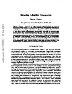
FIGURE 1. Overview of a step in the online adaptive algorithm for finding locally optimal experiments. Top: Method for calculating the utility function U(E), given a simulator and a prior distribution Pr(Θ) over model parameters Θ. Bottom: Method for updating prior distribution with results D from chosen actual experiment.

we suppose that the qubit evolves under an internal Hamiltonian H=

ω σz . 2

Here ω is an unknown parameter whose value we want to estimate. An experiment consists of preparing a single known input state ψin = |+i, the +1 eigenstate of σx , evolving under the Hamiltonian H for a controllable time t and performing a measurement in the σx basis. This is the simplest problem where adaptive Hamiltonian estimation can be used and is the problem studied in reference [5]. In the language of Bayesian inference, the data D ∈ {0, 1} is the outcome of the measurement. An experiment E consists of a specification of time the t that the Hamiltonian is on, while the model parameter Θ is simply ω. The likelihood function is given by the Born rule ω ω Pr(D = 0|Θ, E) = | h+| ei 2 σzt |+i |2 = cos2 ( t). 2 Experimental design is a decision theoretic problem based on the utility function U(t) = ∑ Pr(D|t)

Z

Pr(ω|D,t) log Pr(ω|D,t)dω.

D

The optimal design is any value of t which maximizes this quantity. We proceed by performing the optimal experiment and obtaining data D1 . Using Bayesian inference we update our prior Pr(ω) via Bayes’ rule: Pr(ω|D1 ) =

Pr(D1 |ω) Pr(ω) . Pr(D1 )

If we are not satisfied, we can repeat the process where this distribution becomes the prior for the new experimental design step. This algorithm is depicted in figure 1.

ADAPTIVE HAMILTONIAN ESTIMATION

November 4, 2011

3

Estimators, squared error loss and a greedy alternative to information gain ˆ of The preceding problem had a single unknown variable. If we desire an estimate Θ the true value Θ, the most often used figure of merit is the squared error loss: ˆ = |Θ − Θ| ˆ 2. L(Θ, Θ) ˆ : {D, D1 , D2 , . . . , DN } 7→ R is its expected performance The risk of an estimator Θ with respect to the loss function: ˆ = R(Θ, Θ)

ˆ Pr({D, D1 , D2 , . . . , DN }|Θ)L(Θ, Θ).

∑

{D,D1 ,D2 ,...,DN }

For squared error loss, the risk is also called the mean squared error. The average of this quantity with respect to some prior Pr(Θ) =: π(Θ) is the Bayes risk of π, ˆ = r(π, Θ)

Z

ˆ R(Θ, Θ)π(Θ)dΘ,

and the estimator which minimizes this quantity is called a Bayes estimator. In this case the Bayes estimator is the mean of the posterior distribution1 . Let us assume then that the estimators we choose are Bayes. Let us also choose a uniform prior for Θ. Then, the final figure of merit is the average mean squared error (AMSE): r=

Z

ˆ R(Θ, Θ)dΘ.

We would like a strategy which minimizes this quantity. Non-adaptive Fourier and Bayesian strategies were investigated and compared to an adaptive strategy in reference [5]. Their adaptive strategy fits into the Bayesian experimental design framework when the utility is measured by the variance of the posterior distribution: V (D1 , E1 ) = −

Z

Pr(Θ|D1 , E1 , D, E)(Θ2 − µ(D1 , E1 ))2 dΘ,

where µ(D1 , E1 ) =

Z

Pr(Θ|D1 , E1 , D, E)ΘdΘ

is the mean of the posterior. Recall that the mean is a Bayes estimator of AMSE, so µ = ˆ For a single measurement this utility function satisfies V = −r. That is, maximizing Θ. the utility locally at each step of the algorithm is equivalent to minimizing the AMSE at each step. Hence, when using the negative variance as our utility function, the adaptive strategy summarized in Figure 1 is an example not only of a local optimization, but also 1

Note that in any case where the loss function is strictly proper, i.e. is equal to zero if and only if the estimate is equal to the true state, the Bayes estimator is the posterior mean [6]. ADAPTIVE HAMILTONIAN ESTIMATION

November 4, 2011

4

a greedy algorithm with respect to the AMSE risk. In the future, we shall refer to this choice of utility function together with the local optimization algorithm as the greedy algorithm for this problem. We can write the risk of this strategy recursively as follows. Suppose at the N’th, and final, measurement we have the updated distribution πN−1 . Then, the risk of the local strategy is lN (πN−1 , Θ) = ∑ Pr(DN |Θ, EˆN )L(Θ, µ(DN , EˆN )), DN

where EˆN is the locally optimal design satisfying EˆN = argmin

Z

EN

∑ Pr(DN |Θ, EN )L(Θ, µ(DN , EN )))πN−1(Θ)dΘ. DN

The expected risk at any other stage is ln (πn−1 , Θ) = ∑ Pr(Dn |Eˆn )ln+1



Dn

 Pr(Dn |Θ, Eˆn )πn−1 (Θ) , R Pr(Dn |Θ, Eˆn )πn−1 (Θ)dΘ

where Eˆn is, again, the locally optimal design satisfying Eˆn = argmin

Z

En

∑ Pr(Dn|Θ, En)L(Θ, µ(Dn, En)))πn−1(Θ)dΘ. Dn

Then, the Bayes risk of the greedy strategy is Z

l1 (π0 , Θ)π0 (Θ)dΘ.

Again, it is clear that the greedy algorithm is globally optimal on the final decision, as there is no further hypothetical data to consider. That is, the optimal solution at the N’th measurement is gN (πN−1 , Θ) = ∑ Pr(DN |Θ, EˆN )L(Θ, µ(DN , EˆN )), DN

where EˆN is the locally optimal design satisfying EˆN = argmin EN

Z

∑ Pr(DN |Θ, EN )L(Θ, µ(DN , EN )))πN−1(Θ)dΘ. DN

However, the globally optimal risk at any other stage   ˜n )πn−1 (Θ) Pr(D |Θ, E n gn (πn−1 , Θ) = ∑ Pr(Dn |E˜n )gn+1 R , ˜n )πn−1 (Θ)dΘ Pr(D |Θ, E n Dn where now E˜n is the globally optimal design satisfying   Z Pr(Dn |Θ, En )πn−1 (Θ) ˜ En = argmin ∑ Pr(Dn |Θ, En )gn+1 R πn−1 (Θ)dΘ. Pr(Dn |Θ, En )πn−1 (Θ)dΘ En Dn ADAPTIVE HAMILTONIAN ESTIMATION

November 4, 2011

5

Then, the Bayes risk of the greedy strategy is Z

g1 (π0 , Θ)π0 (Θ)dΘ.

In general, l1 (π0 , Θ) 6= g1 (π0 , Θ). Nor is it the case that Z

l1 (π0 , Θ)π0 (Θ)dΘ =

Z

g1 (π0 , Θ)π0 (Θ)dΘ

for an arbitrary prior. However, for the special case of the uniform prior, we have found numerically that the Bayes risk of the greedy strategy and the Bayes risk of the global strategy are similar enough that the greedy strategy is useful.

Performance comparisons In reference [5], it was shown via simulation that the posterior variance of the greedy strategy is best fit by an exponentially decreasing function of N, the total number of measurements. In contrast, all off-line strategies decrease at best as a linear function of N. In Figure 2, we show that the local information gain optimizing algorithm also enjoys an exponential improvement in accuracy over naive off-line methods. Moreover, we show Nyquist rate sampling is unnecessary and, indeed, sub-optimal. All results stated are obtained using a uniform prior on [0, 1] and are computed numerically by exploring every branch of the the decision tree, in contrast to simulation. In order to be “fair” to the off-line methods, we restricted the adaptive methods to explore the same experimental design specifications. That is, for this particular problem, the adaptive algorithm was allowed to select measurement times from [0, Nmax π], where Nmax is the total number of measurements. In principle, these methods could only do better with a larger design specification.

DISCUSSION Summarizing, we have shown for the problem of estimating the parameter in a simple Hamiltonian model of qubit dynamics an adaptive measurement strategy can exponentially improve the accuracy over offline estimation strategies. Moreover, we have shown that sampling at the Nyquist rate is not optimal in the case of strong measurement. We have derived a recursive solution to the risks for both the local and global optimal strategies. Using this solution, we numerically found that the local strategy is nearly optimal in the special case of a uniform prior. That the greedy algorithm is nearly optimal in a case relevant to experiment demonstrates that an adaptive Bayesian method may be computationally feasible, in that an implementation need not consider all possible future data when choosing each experiment. Together, these results demonstrate the usefulness of an adaptive Bayesian algorithm for parameter estimation in quantum mechanical systems, especially in comparison with ADAPTIVE HAMILTONIAN ESTIMATION

November 4, 2011

6

−1

−1

10

AMSE

AMSE

10

−2

10

−2

10

Nyquist variance Optimized variance Optimized relative entropy Bayes sequential

−3

−3

10

2

4

6

8

10

N

12

10

2

4

6

8

10

12

N

FIGURE 2. Performance of the estimation strategies. The Bayesian sequential and the strategy labeled “Nyquist” sample at the Nyquist rate. The “optimized” strategies find the global maximum utility (using Matlab’s “fmincon” starting with the optimal Nyquist time). In each case, Nmax = 12 measurements are considered. Left: the ideal model discussed in the text. Right: a more realistic model with 25% noise and an addition relaxation process (known as T2 ) which exponentially decays the signal (to half its value at t = 10π).

other algorithms in common use. In the presence of noise, this improvement becomes still more stark, as demonstrated by the results shown in Figure 2. Why is it the case that the Nyquist times are not optimal? First, why should we expect them to be optimal? The Nyquist theorem states that a signal which contains no frequencies higher than ωmax is completely and unambiguously characterized by a discrete set of samples taken at a rate greater than or equal to π/2ωmax . However, the classical notion of sampling fails for the strong-measurement case that we consider here. What we have is a periodic probability distribution which can be sampled, not a periodic function whose values can be ascertained. That is there is no signal, in the classical sense of the word, which can be reconstructed. The failure of the Nyquist rate sampling is exemplified in Figure 3. In this paper, we have chosen to measure success via the squared error loss. Although this is a standard metric, note that it is not practically useful in the context of estimating the parameters of a quantum mechanical system. We motivate this claim as follows. A typical application of our algorithm is to inform control theory algorithms, which can achieve significantly higher fidelities if given a distribution over Hamiltonians rather than a single best estimate. Indeed, in the case of nuclear magnetic resonance, the physical ensemble of qubits produces a real distribution of Hamiltonians to which control theory algorithm must be robust against [7, 8]. Any single estimate of the Hamiltonian parameters will thus artificially exclude dynamics which will appear as decoherence in the resultant pulses. Thus, we must measure the success of our algorithm via a loss function of the true distribution and estimated posterior. Noting that relative entropy is broadly considered the correct loss function for probability estimators, our algorithm, which maximizes expected information gain, becomes the optimal solution. We expect that in more complicated systems, the Bayesian adaptive method will remain useful, especially in applications such as optimal control theory, where having a distribution over Hamiltonians is significantly more useful than a single best estimate. ADAPTIVE HAMILTONIAN ESTIMATION

November 4, 2011

7

100

−0.01 −0.02

60 40 20 0 −20

Before the first measurement After 1 optimal measurement (outcome 0) After 2 optimal measurements (outcomes 0, 1) After 3 optimal measurements (outcomes 0, 1, 0) 0 0.5 1 1.5 2 2.5 3 3.5 4 4.5 5 5.5 6 6.5 7 7.5 8

Negative variance

Information gain

80

−0.03 −0.04 −0.05 −0.06 −0.07 −0.08 −0.09

0 0.5 1 1.5 2 2.5 3 3.5 4 4.5 5 5.5 6 6.5 7 7.5 8

t/π

t/π

FIGURE 3. The information gain (left) and variance (right) utilities for the prior followed by three simulated measurements. The vertical grid lines indicate the Nyquist times. Note that the times at which the utilities are maximized do not necessarily increase with the number of measurements.

ACKNOWLEDGMENTS CF thanks Josh Combes for helpful discussions. This work was financially supported by NSERC and CERC.

REFERENCES 1. T. J. Loredo, AIP Conference Proceedings 707, 330–346 (2004), URL http://dx.doi.org/10. 1063/1.1751377. 2. H. Dreier, A. Dinklage, R. Fischer, M. Hirsch, and P. Kornejew, Review of Scientific Instruments 79, 10E712 (2008), ISSN 00346748, URL http://dx.doi.org/10.1063/1.2956962. 3. U. von Toussaint, T. Schwarz-Selinger, M. Mayer, and S. Gori, Nuclear Instruments and Methods in Physics Research Section B: Beam Interactions with Materials and Atoms 268, 2115–2118 (2010), ISSN 0168-583X, URL http://dx.doi.org/10.1016/j.nimb.2010.02.062. 4. D. V. Lindley, The Annals of Mathematical Statistics 27, 986–1005 (1956), ISSN 0003-4851, URL http://dx.doi.org/10.1214/aoms/1177728069. 5. A. Sergeevich, A. Chandran, J. Combes, S. D. Bartlett, and H. M. Wiseman (2011), URL http: //arxiv.org/abs/1102.3700. 6. R. Blume-Kohout, and P. Hayden (2006), URL http://arxiv.org/abs/quant-ph/ 0603116. 7. N. Boulant, T. F. Havel, M. A. Pravia, and D. G. Cory, Physical Review A 67, 042322+ (2003), URL http://dx.doi.org/10.1103/PhysRevA.67.042322. 8. N. Boulant, J. Emerson, T. Havel, D. Cory, and S. Furuta, The Journal of Chemical Physics 14, 1368+ (2004), URL http://dx.doi.org/10.1063/1.1773161.

ADAPTIVE HAMILTONIAN ESTIMATION

November 4, 2011

8