Adaptive kNN Using Expected Accuracy for Classification of

Adaptive kNN Using Expected Accuracy for Classification of Geo-Spatial Data

arXiv:1801.01453v1 [cs.CV] 14 Dec 2017

Mark Kibanov

University of Kassel, ITeG Center Knowledge and Data Engineering Wilhelmshöher Allee 73 34121, Kassel [email protected]

Martin Atzmueller

Tilburg University (CSAI) Warandelaan 2 5037 AB, Tilburg [email protected]

Martin Becker

University of Würzburg DMIR Group Am Hubland 97074, Würzburg [email protected]. de

Andreas Hotho

University of Würzburg DMIR Group Am Hubland 97074, Würzburg [email protected]

ABSTRACT The k-Nearest Neighbor (kNN) classification approach is conceptually simple – yet widely applied since it often performs well in practical applications. However, using a global constant k does not always provide an optimal solution, e. g., for datasets with an irregular density distribution of data points. This paper proposes an adaptive kNN classifier where k is chosen dynamically for each instance (point) to be classified, such that the expected accuracy of classification is maximized. We define the expected accuracy as the accuracy of a set of structurally similar observations. An arbitrary similarity function can be used to find these observations. We introduce and evaluate different similarity functions. For the evaluation, we use five different classification tasks based on geospatial data. Each classification task consists of (tens of) thousands of items. We demonstrate, that the presented expected accuracy measures can be a good estimator for kNN performance, and the proposed adaptive kNN classifier outperforms common kNN and previously introduced adaptive kNN algorithms. Also, we show that the range of considered k can be significantly reduced to speed up the algorithm without negative influence on classification accuracy.

CCS CONCEPTS • Computing methodologies → Instance-based learning;

KEYWORDS Classification, kNN, Geo-spatial Data, Adaptive Algorithms ACM Reference format: Mark Kibanov, Martin Becker, Juergen Mueller, Martin Atzmueller, Andreas Hotho, and Gerd Stumme. 2018. Adaptive kNN Using Expected Accuracy for SAC 2018, April 9–13, 2018, Pau, France © 2018 Copyright held by the owner/author(s). Publication rights licensed to Association for Computing Machinery. This is the author’s version of the work. It is posted here for your personal use. Not for redistribution. The definitive Version of Record was published in Proceedings of SAC 2018: Symposium on Applied Computing , April 9–13, 2018, https://doi.org/10.1145/ 3167132.3167226.

Juergen Mueller

University of Kassel, ITeG Center Knowledge and Data Engineering Wilhelmshöher Allee 73 34121, Kassel [email protected]

Gerd Stumme

University of Kassel, ITeG Center Knowledge and Data Engineering Wilhelmshöher Allee 73 34121, Kassel [email protected]

Classification of Geo-Spatial Data. In Proceedings of SAC 2018: Symposium on Applied Computing , Pau, France, April 9–13, 2018 (SAC 2018), 9 pages. https://doi.org/10.1145/3167132.3167226

1

INTRODUCTION

(a) Sparse coverage.

(b) Dense coverage.

Figure 1: Examples of different distributions of data points in the WideNoise Dataset. Different colors denote different noise levels. K-nearest neighbors is a simple, yet effective classification algorithm. For example, one of its big advantages is that classification results can be easily interpreted. Consequently, it has been applied in a large variety of settings . The basic assumption of the standard kNN is that a data point (instance) is often a member of the same class as the majority of its k nearest neighbors, where k is fixed for all data points to classify. However, many datasets have an irregular distributions of data points. Consider Figure 1, for example, where areas with different density of points are shown. Due to the density variations, it would be useful to consider different k for different points (items): e. g., a simple intuition would be to use more neighbors in dense areas and less in the areas with sparse neighbors. However, if large k is used, it can be hardly influenced by the largest class; if k is too small, the results can be strongly influenced by a small number of neighbors, e. g., noisy data. Thus, finding an optimal value for k can be a challenging task. In this paper, we address this issue and propose a general approach for an

SAC 2018, April 9–13, 2018, Pau, France adaptive kNN classifier, called ACKER – Adaptive Classifier based on KNN Expected accuRacy). That is, the proposed ACKER algorithm aims to find an optimal k for each point that should be classified. In these terms, an optimal k is defined in such way, that expected accuracy of standard kNN applied to a given point with this k is maximal. To determine the expected accuracy for a point and its k nearest neighbors, we search similar points (in the training dataset) and then compute the accuracy of the kNN classification for them. The set of most similar points can be determined using similarity function. We present different similarity functions and further parameters of ACKER in Section 4 and discuss their influence on the performance of the algorithm in Section 5. In this paper, we concentrate on geo-spatial data to illustrate our approach. For evaluation, we use five different classification tasks, constructed from three datasets with geo-spatial data. We demonstrate the effectiveness of our proposed expected accuracy measure for the algorithm’s predictive performance, and show that the ACKER algorithm outperforms standard kNN and another, previously introduced version of an adaptive kNN algorithm. Finally, we discuss how the number of considered candidate values of k can be reduced to improve the runtime of ACKER. The contributions of this paper can be summarized as follows: (1) We propose a measure for estimating of kNN performance, i.e., the expected accuracy and show its effectiveness. (2) We introduce ACKER and show, that its performance is higher than that of standard kNN and previously introduced version of adaptive kNN. The ACKER algorithm was never introduced before. It is the first time, we explain this algorithm and evaluate it. We use geo-spatial data for the evaluation. This choice is discussed and motivated in Section 3.3. However, we plan to test this approach with more diverse high dimensional data. The rest of the paper is structured as follows. Section 2 discusses related work. Then, we recall some basic concepts in Section 3. In Section 4 we provide a description of the ACKER algorithm and related terms, such as expected accuracy, and similarity functions. The datasets and the results of the evaluation are described in Section 5. Finally, Section 6 concludes the paper with a summary and interesting options for future work.

2

RELATED WORK

The idea of kNN was proposed by Fix and Hodges [5]. Sun and Huang [12] present an adaptive kNN algorithm which aims to select the optimal k for the classification. Kamdar Rajani [6] presented an implementation of this adaptive kNN approach for the MapReduce paradigm. This approach chooses an optimal k based on an optimal k for l nearest neighbors. We compare the proposed adaptive algorithm with ACKER for the presented geo-spatial data. We do not use a MapReduce approach as we make our experiments using 2-dimensional data and thus the runtime is not a critical issue in the presented tasks. Another adaptive kNN approach uses confidence measure to determine an optimal k [10]. Confidence is defined as a share of neighbor items which belong to the majority class. We do not consider this algorithm in our case – because if possible range of

M. Kibanov et al. values of k is {1..n}, then maximal confidence (100%) will be always reached, if k = 1. In this case, either this algorithm is equivalent to standard kNN, or it is necessary to remove some values from Ranдe, e. g., 1. However, in considered datasets, k = 1 was an optimal k for most cases. Thus, we do not use this algorithm as a baseline in this paper. Wang et al. [13, 14] proposed a simple adaptive distance measure for improving the nearest neighbor identification. Ougiaroglou et al. [9] focuses on improving the performance of kNN algorithms by using an adaptive number of nearest neighbors in order to reduce the runtime complexity of the algorithm. In contrast to that, the ACKER concentrates on improving of overall accuracy. In the Section 5.4 we show how to improve the runtime of the ACKER. For the classification, using uncertain information, techniques for reliability-based classification have been developed. Senge et al. [11], for example, present an approach for binary classification that produces a prediction together with a quantification of its reliability. Similar to that approach, the ACKER classifier derives an expected accuracy for classification. Using this parameter, the presented approach can then be tuned in order to provide a prediction that is as exact as possible w.r.t. the given information used for building the model, and for obtaining different classes of the prediction space in terms of the expected accuracy. Many applications can utilize a more accurate kNN classification: e. g., Fang et al. [3] proposed an algorithm for effective join algorithm for trajectory data. That algorithm enables finding nearest Combination of this approach together with our kNN approach may enable new application and algorithms, e. g., for classification of moving objects.

3

BACKGROUND

In this Section, we define the general classification problem, the standard kNN algorithm, and two measures for evaluating the classification quality.

3.1

Classification and kNN Algorithm

We consider the problem of classification. That is, we assume that each point p ∈ P, from a set of points P, can be assigned to a class x ∈ X , from a finite set of classes X , by a classification function c : P → X . The set of all classified points is C = {(p, x) ∈ P ×X | x = c(p)}. In general, the classification function c is unknown. Thus, given a training dataset – a subset of all classified points C train ⊂ C ˆ – the goal is to approximate c by a classification function c. The kNN algorithm results in an approximation cˆk of the classification function c which works as follows: Given a distance function dist : P × P → R, the set Np,k ⊆ T denotes the k nearest neighbors of p in training set C train . We call the pair (p, Np,k ) the k-environment of p (see Section 4.2). The class cˆk (p) assigned to point p is the majority class within this set of k nearest neighbors Np,k . In our particular case we will use geo-spatial points defined by longitude and latitude, i.e., P = [−180; 180] × [−90; 90], and the Euclidean distance function d which approximates the great circle distance well enough for our purposes.

Adaptive kNN Using Expected Accuracy for Classification of Geo-Spatial Data

3.2

Classification Quality Measures

Given an estimated classification function cˆ and a testing set Ct est ⊂ C, Ct est ∩ Ct r ain = ∅, we use the accuracy (acc) as a measure of classification quality. Accuracy is defined as the ratio of correctly classified data points Ct est ∩ Ctcˆest versus the overall number of ˆ data points being classified Ct est , where Ctcˆest = {(p, c(p)) | (p, x) ∈ Ct est } is the set of data points classified by the estimated classifiˆ cation function c: acc(ˆc, Ct est ) =

|Ct est ∩ Ctcˆest | |Ct est |

(1)

Given, a function scorecˆ : P → R that shows a probability or ˆ a score of classification correctness for c(p). We use the Receiver operating characteristic Area Under Curve (ROC AUC) function as measure of the quality of the score function[4]. ROC AUC is defined as follows. Function score predicts, how ˆ is correct. We use expected likely given classification result c(p) accuracy as a score function (see Section 4.2). C t denotes predicˆ ∈ C t , iff tions with score higher than given threshold t: (p, c) ˆ > t. The True Positive Rate function, T PR(t), shows score(p, c) ˆ with score(p, c) ˆ > t is correct: which portion of predictions c(p) T PR(t) =

|C t e s t ∩C tcˆe s t ∩C t | . The False Positive Rate Function,T PR(t), |C t e s t ∩C tcˆes t |

ˆ > t is false: ˆ with score(p, c) shows which portion of predictions c(p) F PR(t) =

|(C tcˆe s t \C t es t )∩C t | . |C tcˆe s t \C t es t |

Then the Receiver operating charac-

teristic, ROC, curve characterizes score function and is defined as follows: ROC(x) = y, iff x = F PR(t) and y = T PR(t). ROC Area Under the Curve (ROC ∫ ∞ AUC) measure quantifies the quality of score: ROC AU C = −∞ T PR(T )(−F PR ′ (T ))dT .

3.3

Discussion

kNN is a basic and well-known classification algorithm that has a number of advantages [8]. First, kNN has no training time, as it is a lazy learning method. kNN can be used as an incremental learner. For some applications, it is important that kNN is easily interpretable. On another side, kNN has disadvantages, some of which are addressed by ACKER, particularly, classification accuracy and tolerance to noise. Further disadvantages, such as the fact that the kNN classification uses more storage space than other algorithms, has low speed of classification and is intolerant to irrelevant attributes, are not critical for the two-dimensional geo-spatial data.

4

ACKER – ADAPTIVE CLASSIFIER BASED ON K NEAREST NEIGHBOUR EXPECTED ACCURACY

The main idea of the ACKER algorithm is to find optimal k for each point (instance) and to use this k with standard kNN, (see Section 4.1). Given a point p, the algorithm estimates the expected accuracy for different possible values of k, and chooses a k that provides a maximum value of the expected accuracy, (see Section 4.2). We apply kNN regression to k-environments of points to estimate the expected accuracy. We use different similarity functions to find the most similar (nearest) points with its k-environments for given point p and its k-environments (see Section 4.3).

SAC 2018, April 9–13, 2018, Pau, France

In this section we describe the proposed classification algorithm and show how the expected accuracy can be computed using different similarity functions. Finally, we discuss the runtime complexity of the algorithm.

4.1

Adaptive k-Nearest Neighbor

We propose an adaptive kNN algorithm – ACKER: Adaptive Classifier based on kNN Expected accuRacy. As mentioned above, the main idea of ACKER is to choose k dynamically for each point to maximize expected accuracy (see Section 4.2). In other words, we need to find k so that exp_acc(p, k) = max {exp_acc(p, k)|k ∈ Ranдe}, where Ranдe is defined as the range of possible values for k. The standard kNN classifier with optimal k is applied afterwards. The ACKER algorithm (see Listing 1) has four input variables: • p is a point for which the classification should be made; • Ranдe ⊆ N defines the set of candidates k. • SimilarityFunction defines which similarity function should be used for estimation of the expected accuracy. • l is the parameter for the expected accuracy estimation (see Equation 2). In addition, the following functions (indicated by teletype font) are used in the algorithm: • expected_accuracy(p, k, SimilarityFunction, l) returns the expected accuracy of kNN for point p and its kenvironment (see Listing 2); • kNN(p, k) returns the result of kNN algorithm for the point p based on k neighbors. Algorithm 1: ACKER Data: point p, set Ranдe, function f , integer l Result: Class of point p 1 optimal_k = 0 2 max_accuracy = –1 3 for k in Range do 4 candidate_accuracy = expected_accuracy(p, k, f , l) 5 if candidate_accuracy > max_accuracy then 6 optimal_k = k 7 max_accuracy = candidate_accuracy 8 end 9 end 10 predicted_class = kNN(p, optimal_k) 11 return (predicted_class) The workflow of the proposed algorithm, Listing 1, can be described, as follows. First, the values of optimal_k and max_accuracy are initialized. The variable optimal_k represents the value of k with the maximal expected accuracy for p found till current iteration; and max_accuracy is the value of that maximal expected accuracy. These variables are initialized with values so, that they are rewritten in the first iteration. The algorithm iterates over all values of k ∈ Ranдe (lines 3 – 9). For each k the algorithms computes an expected accuracy candidate_accuracy (line 4) and compares it with the maximum expected accuracy found previously (lines 5 – 8). The algorithm chooses the k with the highest expected accuracy and

SAC 2018, April 9–13, 2018, Pau, France

M. Kibanov et al.

applies the standard kNN algorithm in order to classify the point (line 10). Next, we discuss, how the expected accuracy can be computed using various similarity functions.

4.2

Expected Accuracy Measure

The intuition behind the expected accuracy can be described as follows. Given a point p with its k-environment, find a set of points Csim,l (p, k) = {p1′ ...pl′ } ⊆ Ct r ain with similar k-environments. As the k-environments are similar, we assume, the accuracy of the kNN-based classification function for given point p, acc(ˆc k (p), {p}), correlates with the accuracy of kNN-based classification function for Csim,l (p, k). So, the expected accuracy is defined as follows: exp_accl (p, k) = acc(ˆc k , Csim,l (p, k))

(2)

Here, we suppose that different regions are statistically similar. Sure, for some data it may be not the case, but in all considered datasets we found that expected accuracy is a good indicator for a real accuracy. Note, that it is necessary to know the correct class for all points p ′ ∈ Csim,l (p, k), i.e. Csim,l (p, k) ⊆ Ct r ain . Listing 2 shows, how the expected accuracy (see Equation 2) can be computed.

4

simavд_dist (p, p ′, k) = −dist(avд_dist(p, k), avд_dist(p ′, k)) (6)

simmax _dist : We denote by max_dist(p, k) the distance to the kth nearest neighbor of the point p: max_dist(p, k) = dist(p, pk )

(7) p′

based on

max_avд_comb(p, k) = (max_dist(p, k), avд_dist(p, k))

(9)

The similarity function based on max_avд_comb is defined as follows:

cor r ectly_pr edict ed l

simmax _avд_comb (p, p ′, k)

Similarity Function

The similarity function sim : P × P × N → R defines, how similar k-environment of two given points are. In some cases, similarity is not dependent on k. We then simply write sim : P × P → R. Consider a function f : P × N → R that characterizes a point and its k-environment. Then, a similarity function based on f can be defined as: (p, p ′, k) 7→ −dist(f (p, k), f (p ′, k)),

here and ∈ P. We introduce three similarity functions sim f . Furthermore, we show, how the previously introduced adaptive kNN [12] can be described using our framework (particularly with a special sim f ). simavд_dist : We denote by avд_dist(p, k) the average distance to the k nearest neighbors of point p: Ík dist(p, pi ) avд_dist(p, k) = i=1 , (5) k here and in the sequel, pi is defined as the ith nearest neighbor to p. The similarity function based on avд_dist is defined as follows:

simmax _avд_comb : We denote by max_avд_comb(p, k) a function that returns a tuple of results of avд_dist (s. Equation 5) and max_dist (s. Equation 7):

expected_accuracy = return (expected_accuracy)

sim f : P × P × N → R

(4)

further p, p ′

simmax _dist (p, p ′, k) = −dist(max_dist(p, k), max_dist(p ′, k)) (8)

Next, we discuss which functions (features of k-environments) can be used to find Csim,l (p, k).

4.3

Csim,l (p, k) = arдmaxpl ′ (sim(p, p ′, k)),

The similarity function for two points p and max_dist is defined as follows:

Algorithm 2: Expected Accuracy Data: point p, integer k, function f , integer l Result: Expected Accuracy for kNN(p, k) ′ 1 Find set C sim,l (p, k) of l different points p with minimal difference to reference function w.r.t. f : sim(p, p ′ ) = | f (p, k) − f (p ′, k)|, Í Csim,l (p, k) = arдmax( sim(p, p ′, k))(see Equation 4) 2 correctly_predicted = number of correct predictions of kNN(p ′, k), where p ′ ∈ Csim,l (p, k) 3

Csim,l (p, k) is defined as the set containing the l points whose k-environments are most similar to the one of p with respect to the given similarity function, also written as

(3)

where dist(x, y) denotes an Euclidean distance. The more similar two points with their k-environments are, the higher is the value of sim f . Note, that the function f can also characterize points and it neighbors by tuple, e. g., f : P × N → R × R, see Equation 9, this does not change the definition of sim f .

= −dist(max_avд_comb(p, k), max_avд_comb(p ′, k))

(10)

lat_lon(p) = (lat(p), lon(p))

(11)

siml at _lon (p, p ′ ) = −dist(lat_lon(p), lat_lon(p ′ ))

(12)

siml at _lon : Sun and Huang [12] introduced an adaptive kNN classifier, where they proposed to choose k which is optimal for l nearest neighbors of point p. We use this approach as a baseline for the evaluation (see Section 5). We set f as follows in order to write adaptive kNN introduced in [12] in ACKER notation: Here, lat_lon(p) are the coordinates (latitude and longitude) of the point. The similarity function based on lat_lon is defined as the Euclidean distance between point and its neighbors: This example shows, how in some cases the ACKER approach can be considered as generalization of other adaptive kNN algorithms. in order to do so, it is necessary to adjust similarity function. The influence of choice of similarity function on overall classification accuracy is shown in the Section 5.3. Next, we discuss

Adaptive kNN Using Expected Accuracy for Classification of Geo-Spatial Data

Table 1: Description of the used datasets

the runtime complexity of ACKER and particularly for computing Csim,l .

4.4

Complexity

We show the runtime complexity of computing Csim,l (and expected accuracy) for given point and its k-environment. Based on that, can we estimate the runtime of the ACKER algorithm. Complexity of finding Csim,l (p, k): If the similarity function is based on function f : P × N → R, the values of f (p), p ∈ Ct r ain can be precomputed offline and indexed using a B+ tree. Given the value of f (p), we need to find Csim,l (p, k). Search in a B+ tree can be done in O(log n), where n is the number of elements of the tree and thus O(log |C train |). The leaves of B+ tree can be linked to each other, so it is necessary to find only one element (which has the nearest value to f (p)) and consider the neighbor elements from it. Thus, the complexity of computing the expected accuracy in this case is O(log |C train |). If f : . . . → R × . . . × R, the kd−Tree should be used instead of B+ tree to index values of f (p), p ∈ P. The search of one element is performed in O(log n) = O(log |C train |). The elements in kd−trees are not linked, so it is necessary to search for l elements, this can be performed in O(l × log |C train |). All steps in Listing 2, except the first line (finding Csim,l ), can be done in O(1). Thus, computing expected accuracy is the same as finding Csim,l (p, k). Complexity of ACKER: In the for–loop (lines 3 – 9 in Listing 1) the expected accuracy should be computed for each k ∈ Ranдe, that means O(|Ranдe | ×log |C train |) or O(|Ranдe | ×l × log |C train |) complexity for the ACKER algorithm, depending on similarity function, as described above. Additionally, it is required to compute values of f (p, k) for all k ∈ Ranдe, where p is the point that should be classified. In worst case, it is necessary to know all k nearest neighbors to compute f (p, k). So, it is needed to find max(Ranдe) nearest neighbors. If the points in training set are indexed using kd−tree, this search is performed in O(max(Ranдe) × loд|C train |). So, the total runtime complexity can be either O(|Ranдe | × log |C train | + max(Ranдe) × loд|C train |) = O((|Ranдe | +max(Ranдe))×log |C train |) = O(max(Ranдe)× log |C train |) , or O(|Ranдe | × l × log |C train | + max(Ranдe) × loд|C train |) = O((|Ranдe | × l + max(Ranдe)) × log |C train |) = O(|Ranдe | × l × log |C train |) , depending on the similarity function sim f as explained above.

5

EVALUATION

We use five different classification tasks with geo-spatial coordinates (latitude and longitude) for evaluation. All presented experiments were conducted using 10-fold cross-validation, where we used each time 90% of the data as training data and 10% of the data as test data. In this section, we describe datasets and classification tasks. We evaluate expected accuracy measure w.r.t. different similarity functions. Finally, we analyze the accuracy of the ACKER classifier and discuss how to optimize the runtime of the ACKER reducing the Ranдe and not decreasing the overall accuracy.

SAC 2018, April 9–13, 2018, Pau, France

Dataset

Geography

Twitter

Milan, Italy

WideNoise SF Crimes

Worldwide San Francisco, CA, USA

5.1

Classes Geographical items mentioned in tweets Measured noise levels Types of crimes

Data

We use three datasets that represent geo-spatial data from three different domains , see Table 1. We constructed five classification tasks, see Table 2, to evaluate the ACKER approach. Here, we shortly present each dataset and classification tasks: Milan Twitter Dataset. The Twitter dataset[1] was collected in Milan between November 1, 2013 and December 31, 2013 for the Telecom Italia Big Data Challenge 2014. For each tweet we consider the entities extracted from the text by the dataTXT-NEX tool 1 : if an entity x is mentioned in tweet, this means that this tweet belongs to the class x. For the classification tasks, twitter8, we consider tweets where one of the seven most popular local geographical items (e. g., “Milan Cathedral”, “Stadium San Siro”) is mentioned. We also added a general entity (“Italy”) in order to add some noise to the data. The second classification task, twitter11, consists of all tweets from twitter8 and tweets with where one of three additional general entities is mentioned. WideNoise Dataset. The WideNoise dataset 2 consists of worldwide noise measurements that were made by mobile app users [2]. We use measurements where GPS-based locations are available. The task is to predict a measured noise level. We test our approach with different number of classes: we divide noise levels into three (widenoise3) and six (widenoise6) classes. The classes in the classification tasks consist of the same number of samples (12,375 measurements per class in widenoise3, and 6,188 measurements per class in widenoise6). San Francisco Crimes Dataset. The San Francisco Crimes dataset consists of all crimes registered by the San Francisco Police Department during 2015. The crime data consists of the location of crimes (coordinates) and crime categories (e. g., “Burglary”, “Drug/narcotic”). The task of the classifier is to predict the crime category, 3

1 https://dandelion.eu/products/datatxt/

2 http://kde.cs.uni-kassel.de/everyaware/dumps/widenoise

3 https://data.sfgov.org/Public-Safety/SFPD-Incidents-Previous-Year-2015-/ritf-b9ki

Table 2: Classification tasks constructed from the datasets Name twitter8 twitter11 widenoise3 widenoise6 crimessf

Dataset Twitter WideNoise SF Crimes

No. of Items

No. of Classes

6,230 21,658 37,126 37,126 149,401

8 11 3 6 16

SAC 2018, April 9–13, 2018, Pau, France

M. Kibanov et al.

given the coordinates of that crime. We consider 16 most popular categories, each with over 1000 incidents in 2015.

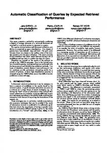
Distribution of types of crimes in crimessf dataset

40000

Expected Accuracy

avg_dist

max_dist

twitter11

20000

10000

IN AL SA U LT LE TH EF VA T N DA LI W AR SM R AN SU BUR TS SP G LA IC RY IO M IS U S SI O N C G C D RU PE R G SO /N N AR C O TI RO C BB SE ER C Y O FR N DA AU RY D W C O EA D ES PO N LA W TR S ES PA SS AS

IC

H

VE

R

IM

SE EN

FF

−C

O

N O

ER

N

R

C

EN

Y/ TH

EF

S

T

0

LA

We evaluate the expected accuracy measure – using the Pearson correlation and the ROC AUC. First, we aim to understand, whether this measure, based on the introduced similarity functions, reflects the real performance of standard kNN. We use the lat_lon similarity function as a baseline. The idea of this similarity function was inspired by [12]. We showed (see Equation 12) that their approach can be presented as a special case of the ACKER algorithm. Still, we use that approach as a baseline. In this (and further experiments) we observe that results for crimessf classification task are different from other classification tasks. We assume, the reason for those differences is a skewed class distribution, (see Figure 2): there are few prevailing classes and many small classes. Over 28% of all items belong to the largest class. Further used datasets have more regular classes frequency. We consider different values of l for evaluation. The variable l defines, how many similar cases should be found to choose k. This number can be chosen manually for given dataset. We discuss some strategies for choosing l in the Section 5.3. Expected accuracies (see Figure 3) generally have a high correlation with the observed accuracy. However, the correlation for small values of l is rather unstable. For both Twitter and WideNoise datasets the expected accuracy based on the proposed similarity functions generally have a higher correlation with the observed accuracy than a lat_lon-based similarity functions. The crimessf classification task is the only exception, where the similarity function based on lat_lon seems to perform best. Generally, the correlations strongly depend on choice of l.

30000

O TH

5.2

Number of commited crimes

Note, we did all of the following experiments for all five classification tasks for k ∈ {1..200} and l ∈ {1..1000}. Due to space constraints, we do not outline redundant results: e.g., if only a plot for widenoise6 is shown, it means, the plot for widenoise3 has the same learnings; or if a plot for k = 10 is shown, plots for other values of k have the same tendencies.

Types of crimes

Figure 2: Frequency of different crimes in crimessf classification task.

Next, we compute the ROC AUC values for the same experiments to check if the expected accuracy measure is a good predictor of whether standard kNN classifies correctly. Figure 4 shows the ROC AUC scores values dependent on the different similarity functions and values of l for the considered classification tasks. Overall, the similarity function performs as a good predictor for correctness of standard kNN classification. The expected accuracy performs better than a random predictor (ROC AUC > 0.5). moreover, expected accuracy, based on lat_lon similarity function, performs very well in terms of ROC AUC if the value of l is low (it reaches almost 90% for the Twitter dataset).

max_avg_comb

lat_lon

widenoise6

crimessf

Correlation Coefficient

1.00 0.75 0.50 0.25 0.00 −0.25 0

250

500

750

1000

0

250

500

750

1000

0

250

500

l−Value

Figure 3: Correlation between real and expected accuracy dependent on value of l

750

1000

Adaptive kNN Using Expected Accuracy for Classification of Geo-Spatial Data avg_dist

max_dist

twitter11

SAC 2018, April 9–13, 2018, Pau, France

max_avg_comb

lat_lon

widenoise6

crimessf

ROC AUC Score

1.00 0.90 0.80 0.70 0.60 0.50 0

250

500

750

1000

0

250

500

750

1000

0

250

500

750

1000

l−Value

Figure 4: ROC AUC scores of expected accuracy of standard kNN for k = 200.

Adaptive kNN

In contrast, for the crimessf classification task, only the ACKER with the lat_lon-based similarity function shows an improvement in terms of accuracy compared to the standard kNN. However, this improvement is marginal. This is the only classification task, where the proposed similarity functions performed poorer than the baseline. For all classification tasks the choice of l and similarity function is very important: e. g., for the classifier with the avд_dist-based similarity function of twitter11 the minimal accuracy is 69.5% (with l = 27) and the maximal accuracy is 81.4% (with l = 268). How to choose an optimal similarity function and l? In the previous section we considered two popular measures to estimate the relevance of expected accuracy – correlation coefficient and ROC AUC. The experiments results show that correlation coefficient is a much better indicator for choosing an optimal l and similarity function. For the four classification tasks accuracy of the ACKER based on lat_lon similarity function performs poorer than ACKER based on the other functions; and vice versa for the crimessf classification task. The same observations can be found in correlation between expected accuracy and observed accuracy (s. Figure 3 and Figure 6): correlation coefficient with lat_lon-based expected accuracy is lower than with other expected accuracies for WideNoise and Twitter datasets and vice versa for San Francisco Crimes Dataset. In terms of ROC AUC, the lat_lon-based expected accuracy performed best for all classification tasks (see Figure 4). Considering l, it is necessary to notice that the ACKER algorithm

widenoise3

50

100

k

150

200

0

50

100

k

150

200

crimessf

Accuracy

0.30

0.32

Accuracy

0.54

0.34

0.56 0

0.52

Accuracy

0.65

0.50

0.70

Accuracy

0.75

0.80 0.75 0.70 0.65

Accuracy

widenoise6 0.36

twitter11

0.85

twitter8

0

50

100

k

150

200

0

50

100

k

150

200

0.22 0.24 0.26 0.28 0.30 0.32

Next, we discuss the performance of standard kNN and ACKER in terms of classification accuracy. Figure 5 shows the mean accuracy and its standard deviation of standard kNN algorithm dependent on the choice of k. All classification tasks have different accuracy (note different Y-axis scales) as they have different number of classes, points and classes distribution. For Twitter and WideNoise datasets, the standard kNN classifier performs best if k is low. Its accuracy decreases if k increases. In contrast, standard kNN with crimessf shows the worst performance with low k (in fact, if k is low, even choosing the most popular class performs better). Standard kNN performs best for crimessf with k = 69. For all classification tasks, the standard deviation is rather low, the results of standard kNN are stable. We implemented the ACKER algorithm, as described in Listing 1. Figure 6 shows, how the accuracy for different datasets depends on the parameter l. Here, again, the results for crimessf classification task differ from the results for other classification tasks. First, consider the Twitter and WideNoise classification tasks: ACKER outperforms the standard kNN classifier, for the most l, e. g., the best possible accuracy for twitter11 using standard kNN (with optimal k) is 77.3%, and the accuracy of ACKER (for max_avд_comb with optimal l) is: 82.5%. Also, the ACKER algorithm with introduced functions outperforms the baseline (we use adaptive kNN classification introduced in [12] as a baseline).

0.28

5.3

0

50

100

150

200

k

Figure 5: 10-fold cross-validation mean accuracy and standard deviation of common kNN classifier dependent on value of k

SAC 2018, April 9–13, 2018, Pau, France

M. Kibanov et al.

avg_dist twitter8

max_avg_comb

lat_lon

twitter11

max_dist

common kNN

widenoise3

widenoise6

crimessf

0.58 0.37

0.80

0.56 0.55

Accuracy

0.76

0.36

Accuracy

Accuracy

Accuracy

Accuracy

0.82

0.32

0.57

0.84

0.35 0.34

0.54

0.72

0.30 0.28 0.26

0.33 0.53

0.80 0

250

500

750

1000

0

250

l−Value

500

750

1000

0.24 0

250

l−Value

500

750

1000

0

250

l−Value

500

750

1000

0

l−Value

250

500

750

1000

l−Value

Figure 6: Accuracy of the ACKER classifier dependent on the number of considered similar points l performs better with higher values of l, the same as correlation coefficient is much stable with higher values of l. Again, ROC AUC values (see Figure 4) were lower with higher l for all classification tasks. Thus, ROC AUC could not predict performance of similarity function and l. We conclude with some recommendations about the choice of the similarity function and l. One way to determine an optimal combination of similarity function and l is to use the training dataset to calculate correlations between expected and real accuracy and analytically determine optimal similarity function and value of l. It is also worth noticing that in many of our experiments the max_avд_comb-based ACKER classifier performs best: it has the best accuracy if an optimal l is chosen in most scenarios.

5.4 Choice of Range of k In the previous sections, we discussed the performance of ACKER for different similarity functions and numbers of considered similar points l. However, we did not discuss the choice of value of Ranдe, see Listing 1. In all previous experiments we used Ranдe = {1..200}. Since it is necessary that ACKER iterates over the Ranдe, the runtime complexity of the ACKER algorithm is linearly dependent on number of values in Ranдe, |Ranдe |, see Section 4.4. Here we discuss, whether it is possible to reduce Ranдe in order to speed up the runtime of ACKER.

avg_dist

In this experiment, for each classification task and each similarity function, we use fixed value of l, and particularly the value which performs best with Ranдe = {1..200}, see Table 3. We evaluate, how the ACKER algorithm performs with different ranges of k, Ranдe = {1..kmax }, where kmax ∈ 1..200. As in previous experiments, we use the accuracy of the algorithm for evaluation – Figure 7 shows dependency of accuracy on kmax . Note, if kmax = 1, the algorithm is equivalent to the standard kNN with k = 1, and if k = 200, it is equivalent to the results discussed in Section 5.3. For low values of kmax even small increase of kmax improves the accuracy of the ACKER classification for all classification tasks. Increasing kmax if kmax ≥ 50, does not increase the accuracy of ACKER for any classification task or similarity function, and even Table 3: Optimal values of l (in terms of accuracy) for the considered classification tasks and similarity functions Class. Task

avд_dist

max_avд_comb

lat_lon

169 251 873 968 734

175 268 829 854 742

113 191 1000 799 290

1 1 298 379 166

twitter8 twitter11 widenoise3 widenoise6 crimessf

max_avg_comb

twitter11

max_dist

lat_lon

max_dist

widenoise6

crimessf 0.33

0.80 0.79

0.37

Accuracy

0.81

Accuracy

Accuracy

0.82

0.36

0.30 0.28 0.25

0.78 0.23 0

50

100

kmax

150

200

0

50

100

kmax

150

200

0

50

100

150

200

kmax

Figure 7: The accuracy of ACKER classifier dependent on value of kmax and different similarity functions

Adaptive kNN Using Expected Accuracy for Classification of Geo-Spatial Data vice versa: e. g., consider avд_dist-based similarity function for widenoise6. It reaches maximum accuracy with kmax = 41. These observations correspond with Figure 5: for the standard kNN algorithm the accuracy decreases if k increases (Twitter and WideNoise), or does not change much after certain k (San Francisco Crimes Data). The ACKER algorithm needs some number of k values in Ranдe to be able to “choose” from, but after certain value of kmax the accuracy does not improve. For the choice of kmax , we suggest to use a visual elbow rule based on experiments as in Figure 5, as it is common for clustering algorithms [7].

6

CONCLUSIONS AND FUTURE WORK

In this paper, we presented an adaptive kNN classification algorithm – the ACKER algorithm. The basic idea of the algorithm is to choose k for each item by maximizing its expected accuracy. Expected accuracy is computed based on similar points. We introduced three different similarity functions, and used method introduced by Sun and Huang [12] as the baseline. The evaluation was conducted using five different classification tasks, derived from three different datasets with geo-spatial data. The proposed ACKER algorithm based on three introduced similarity functions showed clear accuracy improvement compared to the standard kNN algorithm and to previously introduced adaptive kNN algorithms for the most classification tasks. The only dataset, for which ACKER could not improve the accuracy compared to standard kNN was San Francisco Crimes Dataset. One possible explanation, kNN approach can not perform well with this dataset, is a skewed class distribution. Moreover, the expected accuracy demonstrated a fair ability to predict classification correctness, reaching ROC AUC of over 0.9 for some classification tasks and high correlation values with the observed accuracy. Further, we showed, it is not necessary to consider a large Ranдe of k values, as after some point, additional ks do not improve an accuracy. Particularly, reducing Ranдe from 200 elements to 50 elements does not decrease accuracy, but can reduce runtime by four times (as it linearly depends on max(Ranдe), or |Ranдe |). The presented approach is able to improve classification using the topology of data. This is simple approach. Further, it is possible to consider the variability of considered phenomena for different problems. This is a possible way to extend the method. In this case, it would be necessary to make expected accuracy dependent on further factors. Another promising topic for the future work is a more detailed investigation of different similarity functions and their influence on the expected accuracy. Also, we aim to apply the classifier on non-geo-spatial data in order to test its ability to work with multidimensional data. We discussed some heuristics to choose the right parameters for ACKER. However, more formal approaches for the choice of the input parameters of ACKER could be very useful for future applications.

REFERENCES

[1] Gianni Barlacchi, Marco De Nadai, Roberto Larcher, Antonio Casella, Cristiana Chitic, Giovanni Torrisi, Fabrizio Antonelli, Alessandro Vespignani, Alex Pentland, and Bruno Lepri. 2015. A multi-source dataset of urban life in the city of Milan and the Province of Trentino. Scientific Data 2 (Oct. 2015), 150055. https://doi.org/10.1038/sdata.2015.55

SAC 2018, April 9–13, 2018, Pau, France

[2] Martin Becker, Saverio Caminiti, Donato Fiorella, Louise Francis, Pietro Gravino, Mordechai (Muki) Haklay, Andreas Hotho, Vittorio Loreto, Juergen Mueller, Ferdinando Ricchiuti, Vito D. P. Servedio, Alina Sîrbu, and Francesca Tria. 2013. Awareness and Learning in Participatory Noise Sensing. PLOS ONE 8, 12 (2013). https://doi.org/10.1371/journal.pone.0081638 [3] Y. Fang, R. Cheng, W. Tang, S. Maniu, and X. Yang. 2016. Scalable Algorithms for Nearest-Neighbor Joins on Big Trajectory Data. IEEE Transactions on Knowledge and Data Engineering 28, 3 (March 2016), 785–800. https://doi.org/10.1109/TKDE. 2015.2492561 [4] Tom Fawcett. 2006. An Introduction to ROC Analysis. Pattern Recogn. Lett. 27, 8 (June 2006), 861–874. https://doi.org/10.1016/j.patrec.2005.10.010 [5] Evelyn Fix and Joseph L Hodges Jr. 1951. Discriminatory analysis-nonparametric discrimination: consistency properties. Technical Report. California Univ Berkeley. [6] B Apexa Kamdar and K Ishan Rajani. 2015. Improved Adaptive K Nearest Neighbor algorithm using MapReduce. International Journal of Science, Engineering and Technology Research (IJSETR) 4, 6 (2015). [7] David J. Ketchen and Christopher L. Shook. 1996. The Application of Cluster Analysis in Strategic Management Research: an Analysis and Critique. Strategic Management Journal 17, 6 (1996), 441–458. https://doi.org/10.1002/(SICI) 1097-0266(199606)17:63.0.CO;2-G [8] S. B. Kotsiantis. 2007. Supervised Machine Learning: A Review of Classification Techniques. Informatica 31, 3 (2007). http://www.informatica.si/index.php/ informatica/article/view/148 [9] Stefanos Ougiaroglou, Alexandros Nanopoulos, Apostolos N. Papadopoulos, Yannis Manolopoulos, and Tatjana Welzer-Druzovec. 2007. Adaptive k-NearestNeighbor Classification Using a Dynamic Number of Nearest Neighbors. In 11th East-European Conference on Advances in Databases and Information Systems (ADBIS 2007). Springer, 66–82. https://doi.org/10.1007/978-3-540-75185-4_7 [10] Vandana Roy and Sriganesh Madhvanath. 2008. A Skew-tolerant Strategy and Confidence Measure for k-NN Classification of Online Handwritten Characters. Technical Report 4. Tech. rep., HP Laboratories. 48. [11] Robin Senge, Stefan Bösner, Krzysztof Dembczynski, Jörg Haasenritter, Oliver Hirsch, Norbert Donner-Banzhoff, and Eyke Hüllermeier. 2014. Reliable Classification: Learning Classifiers that Distinguish Aleatoric and Epistemic Uncertainty. Inform. Sci. 255 (2014), 16–29. https://doi.org/10.1016/j.ins.2013.07.030 [12] Shiliang Sun and Rongqing Huang. 2010. An Adaptive k-Nearest Neighbor Algorithm. In 7th International Conference on Fuzzy Systems and Knowledge Discovery (FSKD 2010), Vol. 1. IEEE, 91–94. https://doi.org/10.1109/FSKD.2010. 5569740 [13] Jigang Wang, Predrag Neskovic, and Leon N. Cooper. 2006. Neighborhood Size Selection in the k-Nearest-Neighbor Rule Using Statistical Confidence. Pattern Recogn. 39, 3 (2006), 417–423. https://doi.org/10.1016/j.patcog.2005.08.009 [14] Jigang Wang, Predrag Neskovic, and Leon N. Cooper. 2007. Improving Nearest Neighbor Rule with a Simple Adaptive Distance Measure. Pattern Recogn. Lett. 28, 2 (2007), 207–213. https://doi.org/10.1016/j.patrec.2006.07.002