Adaptive Lossless Prediction based Image Compression

Appl. Math. Inf. Sci. 8, No. 1, 153-160 (2014)

153

Applied Mathematics & Information Sciences An International Journal http://dx.doi.org/10.12785/amis/080119

Adaptive Lossless Prediction based Image Compression Raka Jovanovic1,2,∗ and Rudolph A. Lorentz3 1 Institute

of Physics, University of Belgrade,Pregrevica 118, Zemun, Serbia Environment and Energy Research Institute (QEERI), Qatar 3 Texas AM University at Qatar, Doha, PO Box 23874, Qatar 2 Qatar

Received: 4 Jun. 2013, Revised: 18 Sep. 2013, Accepted: 19 Sep. 2013 Published online: 1 Jan. 2014

Abstract: Predictive methods of image compression traditionally visit the pixels to be compressed in raster scan order, making a prediction for that pixel and storing the difference between the pixel and its prediction. We introduce a new predictive lossless compression method in which the order in which the pixels are visited is determined using a predictor based on previously known pixel values. This makes it possible to reconstruct the image without storing this path. In our tests on standard benchmark images; we show that our approach gives a significant improvement to row wise use of one or two dimensional predictors and gives results similar to or better than standard compression algorithms like median compression and JPG 2000. Keywords: Image Compression, Adaptive, Prediction methods.

1 Introduction Since computers have been used for presenting multimedia, image compression has been widely used and researched. The two main directions of this research where lossy and lossless compression. Although the lossy approach gives significantly greater compression ratios, it does not give acceptable results for applications like medical imaging, image archiving,and remote sensing, which require or desire lossless compression. The purpose of this article is to introduce a new approach to lossless image compression. Although we describe and test it on images, it could also be used for data on irregular grids as long as there is information available on the proximity of the data points. A wide range of algorithms for image compression have been developed. Today the most commonly used formats are JPG LS [1], and JPEG2000 [2], due to it’s speed and sufficiently good compression ratios. Significantly, more complex algorithms like CALIC [3], TMW[5] and EDP [4] have been developed for improved compression ratios. Except for JPEG2000 which uses a wavelet transform, all the other methods mentioned use a prediction approach. This means making a prediction for the pixel to be compressed and storing the difference between the pixel and its prediction (the error), and later compressing them using some encoding method like ∗ Corresponding

Huffman, Rice or arithmetic. In this approach, the idea is to predict the value of a pixel using previously visited neighbors. JPG-LS implements the LOCO-I algorithm, in which the prediction is based on three neighboring points and context modeling which is used for recognizing local activity like smoothness and texture patterns. CALIC uses a more complex context based adaptive method which uses a large number of modeling states to condition a nonlinear predictor and adapt the predictors to varying source statistics. TMW extends this approach by adding an image analysis stage which extracts some global image information that is used to improve the quality of the predictions. EDP uses an edge direct prediction approach using a large number of neighboring points. All of the previously mentioned methods improve their compression ratios by using more complex formulas for predicting the value of image pixels. These algorithms have in common that they go through image in raster scan order, that is row by row. The PNG (Portable Network Graphics) [6] image format uses Adam7, an interlacing algorithm which changes the order in which the pixels are visited. However, this changed order is not used to improve compression but to make it possible to view the image even when not all of the data has been transferred by the network (progressive scan). In this article we present a novel approach in which we use a simple nearest neighbor predictor, but we increase

author e-mail: [email protected] c 2014 NSP

Natural Sciences Publishing Cor.

154

R. Jovanovic, R. Lorentz: Adaptive Lossless Prediction based Image Compression

the compression ratio by the order in which we visit the pixels of the image or in other words selecting a different path for our predictions. Our method consists of three parts. The first is a predictor for the value of a pixel which could potentially be compressed. The second is a predictor for the error that would be made by using the value predictor. The error predictor is applied to all pixels whose error can be predicted from already compressed pixels. The third is an optimization: compress that pixel for which the absolute value of the predicted error is the smallest among all pixels to which the error predictor can be applied. We show in our results, that the use of this algorithm greatly improves the compression ratios achieved by the simple use of a one dimensional predictor and storing the differences. We show that it gives results similar to JPEG2000, and even has better results in the case of gray scale 16 bit images. This paper is organized as follows. In Section 2, we present our algorithm for path creation. In Section 3, we focus on the implementation details of our algorithm. In Section 5, we analyze and compare the results obtained by using our compression method to previously mentioned methods on standard benchmark images.

2 The Idea of the Algorithm As previously mentioned, all of the widely adopted prediction based compression algorithms for image compression go through the image in raster scan order, or in other words row by row. The advantage of this approach is that only a small of number of pixels needs to be buffered and, as a consequence of this, a relatively small amount of memory is needed. We present a new approach to data compression in which we do not increase our compression ratio by using a better prediction function, but by choosing in which order the pixel values will be compressed. Predictive methods achieve compression because the difference between pixel values and their predictions are generally smaller numbers than the pixel values themselves and therefore need less space to store. If when going from one compressed pixel to the next, we have the freedom which of its neighbors will be compressed next, we can chose that neighbor for which the difference between pixel value and predictor is the smallest. Thus the idea is that, at each step of the algorithm, we predict the pixel with the smallest possible error of all the possible directions. This is a similar concept to Prim’s algorithm to finding the minimal spanning tree of a weighted graph - the weights being the absolute values of the errors - using a depth first search [7]. It is not quite the same, since in our approach we implicitly determine a spanning tree via a breadth first search on a weighted graph whose weights could change during the course of the calculations. Due to the nature of predictive compression, a prediction must be calculated using only the values of

c 2014 NSP


previously predicted pixels. Otherwise the compressed values cannot be decompressed. One way to get around this is to store the order in which the pixels are compressed as well as the direction from which the prediction came. Even in the case of only four possible directions (up, down, left and right), we have two extra bits for each pixel. In our algorithm, instead of storing the path we have used to compress the image, we use a predictor for calculating the error between an uncompressed pixel and a neighboring compressed pixel. This heuristic is based on only already compressed pixels. Then, at each step of the algorithm, we look for that pixel with the smallest estimated error in some direction and compress that pixel. In this article we use the following notation: X for the image being compressed, xi, j corresponds to the value of the pixel an position (i, j). We use D = (Dx, Dy) to denote a direction. The four possible directions up, down, left and right are the vectors (1,0), (-1,0), (0,1) and (0,-1). The simplest method of compressing the pixels of an image in raster scan order is to take the difference between the current pixel and the previous one (except for the first pixel in a row). If the current pixel is xi, j that neighboring pixel will be denoted by N(xi, j ) = xi−1, j−1 . The neighboring pixel from direction D is NE(xi, j , D) = xi−Dx,i−Dy

(1)

The basic idea of our algorithm is that at each step we predict the pixel with the smallest possible error using NE, which is the same as finding that xi, j and that D for which |xi, j − NE(xi, j , D)| is minimal. The smallest error can only be determined if we know the values of pixels that can be predicted, which is not possible in the phase of decompression. Instead we use a heuristic approach in which the error of predicting xi, j , from xi−Dx, j−Dy is replaced by predicting xi−Dx, j−Dy from xi−2Dx, j−2Dy . Thus we replace the search for that pixel xi, j and direction D for which |xi, j − NE(xi, j , D)| is minimal by the search for that pixel xi, j and direction D for which |xi−Dx, j−Dy − NE(xi−Dx, j−Dx , D)| is minimal. Note that NE(xi−Dx, j−Dx , D) = xi−2Dx, j−2Dy . There is no error in this replacement if the image intensities are linear in the direction D for the pixels involved. Finally, once xi, j and D have been determined, the difference xi, j − NE(xi, j , D) is computed and encoded. This type of heuristic is defined for a position P, direction of prediction D and its value is xP − NE(xP , D). It can be used for predictive compression only if the pixels xi−Dx, j−Dx and xi−2Dx, j−2Dy have already been compressed. We consider a prediction available if pixels at positions xi−Dx, j−Dy and xi−2Dx, j−2Dy have been previously visited. We define the following function

α (P, D) = xP − NE(xP , D)

(2)

For simplicity we shall define E as a set of pairs of position and direction (P, D), which defines a prediction

Appl. Math. Inf. Sci. 8, No. 1, 153-160 (2014) / www.naturalspublishing.com/Journals.asp

155

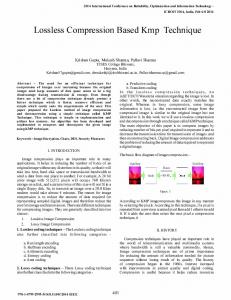
Fig. 1: A) Initialization: storing 4 values from the top left corner, B) First step: moving from (1,0) left to (2,0) storing the value x2,0 − x1,0 , C) Second step: moving from (0,1) down to (0,2) storing the value x0,2 − x0,1 , D) Third step: moving from (1,1) left to (2,1) storing the value x2,1 − x1,1

and extend α to this set. Now we can more precisely say that at each step k of our algorithm we wish to use prediction ei ∈ Mk , where Mk ⊂ E, is a set of all available predictions at step k, with the smallest value of α (ei ) NextPrediction = arg min α (ei ) ei ∈Mk

(3)

3 Basic Version of the Algorithm To implement the idea explained in the previous section, we need to define several structures. First we define ∆ as the output array in which we store differences between the predictions and original values. We will also need a structure that stores possible predictions e ∈ E with corresponding values of α which we shall denote as WaitList. WaitList should be a an ordered list sorted by α . We shall also need a structure Covered that tracks which pixels have previously been predicted. The algorithm is divided into the initialization, and iteration steps. In the initialization step we take the top left 2 ∗ 2 square write those values to the output array ∆ , and calculate predictions for the 4 neighboring points, sort them by difference and add to WaitList(see Figure 1A).

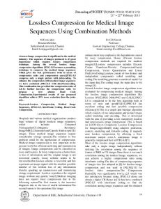
An iteration step can be divided into two stages, first removing the element with the best value of heuristic e from the WaitList. We use it to predict the corresponding element xe if it is not already covered, and store the error of prediction to the output array ∆ . The second is updating the WaitList. We add the new predictions that can be made using xe and its neighboring points to appropriate positions in the sorted WaitList. We finally update Covered. An example of this algorithm can bee seen in Figure 1. The heuristic function α does not have any kind of edge detection, which is a significant weakness. We improve the the quality of α for predicting point x from point p with direction D by taking into account how good the prediction of neighboring points of x in the same direction D. The neighboring points (NP) that are taken into account can be seen from Figure 2. To do this we first define an extension of α

α0 (P, D) = Covered(P, D) ∗ α (P, D)

(4)

In Equation 4, Covered(P, D) is 1 if the prediction from P in direction D can be made, and 0 if not. We use α0 to declare a function that defines the influence of neighboring points of x to the heuristic value. We can

c 2014 NSP


156


In the decompression algorithm, the initialization is done using the first 4 elements from ∆ for the known starting position. The second correction is that instead of calculating the prediction error using the original image, we load it from the current position of the input buffer. Using the new value we advance to the new position and use it to reconstruct the pixel that is predicted by e. When adding new elements to the wait list, only covered points are used.

4 Implementation Fig. 2: Example of in the improved heuristic. The pixel X is predicted in the down direction

define the improved heuristic function αe q(p, D) = 1 +

∑

(Covered(i, j) ∗ ai, j )

(5)

(i, j)∈NP

αe (P, D) =

α (P, D) + ∑(i, j)∈NP (α0 (i, j, D)) q(P, D)

(6)

In Equation 5, ai, j is the coefficient at appropriate position which can be seen from Figure 2. We used the following values a0 = 1, a1 = 0.75 and a2 = 0.5. The use of the new heuristic function αi changes the algorithm slightly due to the fact that when we take an element from the WaitList, it is possible that the value of αi has changed because new points have been covered. The algorithm changes in the following way: when e is taken from the WaitList, we first check if the value of αi (e) has changed and if it has increased, we return e with the new value of αi to the WaitList at the appropriate position. This algorithm has the following pseudo code Delta.Reset(); mWaitList.Initialize(Image); while Not(mWaitList.Empty()) do e = mWaitList.TakeFirstElement(); nHeuristic = CalculateHeuristic(e); if (nHeuristic > e.Heuristic) then e.Heuristic = nHeuristic; mWaitList.AddNewElementLIFO(tElement); else NewPos = e.PredictionPosition if Not(Covered(NewPos)) then Error = e.PredictionError(Image); Delta.AddToPath(Error); mWaitList.AddExtraElements(NewPos, Covered,Image); end if end if end while

c 2014 NSP


In this section, we clarify some details of the implementation. First we wish to mention that we did not use signed integer numbers for storing the errors but unsigned integer values. We have done this conversion through the prediction error mapping function as explained in [8]. We encode the prediction error with the SZIP compression algorithm [9] which implements an enhanced version of Rice encoding. As mentioned in the previous section, WaitList is a sorted doubly connected list. Adding elements to a sorted list is time consuming and in general has a complexity asymptotically equal to its length l. In our algorithm, the list is used only in two ways: removing the first element, and adding new elements to appropriate positions. When adding a new element with an error that is equal to some elements that already exist in the list, we use the first in last out (FILO) approach. We have decided to use FILO instead of first in first out (FIFO) because in a large number of tests we have conducted, it gave a greater compression ratio after encoding. Because of the way the list is used, and knowing that all the possible values are bounded, made it possible to add elements in nearly constant time, or more precisely bounded by a constant independent of the size of the image being compressed. We have done this by adding an extra array that can hold all the possible values of errors. Each array element is a pair of the first element with the appropriate error start and the last one end. Adding a new element with error i is know equivalent to setting it as the start of i-th array element and performing the necessary reconnections of list elements. The complexity of the calculations is asymptotically equivalent to the size of image n. Each pixel is predicted only once, but in the worst case scenario up to 4 predictions can be added to the Waitlist. The predictions that are not used can easily be disregarded due to the tracking of covered pixels and do not significantly effect the over all calculation time. The calculation of the αi is optimized by storing the values of α . The repeated storing of predictions to the WaitList, in the worst case, can be done up to 3 times, which doesn’t change the asymptotical calculation time. The storage complexity of the algorithm is equivalent to n. We need to have memory for holding the image X and for tracking the covered pixels for which we need need n times a constant. The


157

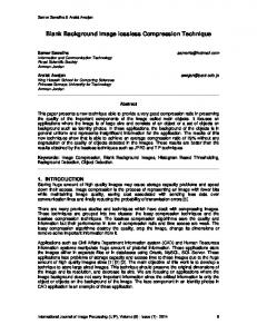
Fig. 3: Example of predictions being used in the improved heuristic. Small prediction errors are shown as dark, and high errors are shown as bright

WaitList only holds the border elements of the covered region, because of which it is always smaller than n.

5 Results We compare the effectiveness of our algorithm to compression ratios achieved by one or two dimensional linear extrapolation as predictions and the median edge detection predictor [10] using raster scan (row by row) order. We also compare our results with JPG2000 as a standard in image compression. We have conducted our experiments using the standard Kodak images for 8 bit grey scale, which we downloaded from the Rich Franzen web site [11]. We have also done tests on 16 bit grey scale benchmark images which we have taken from the

compression database web site [12]. The JPEG2000 plugin for Adobe PhotoShop was used to get the values for 16 bit JPG2000 compression in Table 2. We have implemented our algorithm using Microsoft Visual Studio 2008 and have written the code in C#. The values for one dimensional, two dimensional and median predictors are calculated by our own software using the well know formulas and using the same SZIP for encoding. The results in tables 1, 2 show the compression in bits per pixel for each of the methods. The results in Table 1 for 8 bit images were computed as follows. 1D is a one dimensional predictor, which runs through the image in raster scan order from top to bottom and uses the previous pixel as a prediction for the next pixel. The 2D predictor runs through the image the same

c 2014 NSP


158


Table 1: Comparison of compression ratio for 8 bit grey scale images in bits per pixel File

X*Y

1D

2D

MED

JP2

AD

kodim01 kodim02 kodim03 kodim04 kodim05 kodim06 kodim07 kodim08 kodim09 kodim10

768*512 768*512 768*512 512*768 768*512 768*512 768*512 768*512 512*768 512*768

5.86 4.51 3.94 4.78 5.86 4.79 4.29 6.14 4.59 4.69 4.95

5.63 4.53 4.03 4.60 5.70 5.10 4.16 5.65 4.52 4.52 4.84

5.36 4.24 3.75 4.33 5.52 4.81 3.93 5.41 4.20 4.23 4.58

5.45 4.19 3.56 4.20 5.32 4.69 3.77 5.54 4.02 4.10 4.48

5.45 4.20 3.68 4.38 5.33 4.78 3.86 5.48 4.17 4.20 4.55

Table 2: Comparison of compression ratio for 16 bit grey scale images in bits per pixel File

X*Y

1D

2D

MED

JP2

HO

cr rtg jb im branches im flower im town im kid mr 2321

612*746 819*536 819*536 821*536 824*540 512*512

11.54 14.03 10.56 12.41 12.40 11.88 12.14

11.31 14.02 10.30 12.52 11.65 11.47 11.88

11.06 13.77 10.15 12.29 11.54 11.43 11.71

11.22 14.17 10.11 12.52 11.67 11.31 11.83

11.07 13.66 10.01 12.12 11.48 11.45 11.63

way and predicts the next pixel value by a linear extrapolation from the neighboring pixels to the West, to the Northwest and to the North of the pixel to be compressed. MED is the median predictor which uses the same pixels as the 2D predictor, but uses a formula which takes into account possible edges (see [10]). Our method is denoted AD. We see that by using a different order and direction of the 1D predictor we get a significant decrease of 10% in bits needed to store the image. Our algorithm gives similar, slightly better results than the use of the median predictor. This is unexpected due to the fact that the median changes it’s predictor function from one dimensional in X,Y directions if an edge is expected, and a two dimensional otherwise, whereas our algorithm only uses one dimensional predictions. Our algorithm performs similar slightly to, but slightly worse, than the standard compression JPEG 2000. We have to mention that the results used for JPG2000 are slightly worse than they could have been due existence of an additional header in the compressed files. In the case of 16 bit images we have similar results, with our algorithm giving results that are slightly better that JPG2000. We believe that increased compression ratio of our simple one dimensional predictor is due to the adaptability of using predictions in the X or Y direction.

c 2014 NSP


A second factor is that our algorithm tends to group first areas with small prediction errors and later areas with high errors. This makes the data better prepared for the encoding stage. We can see the order in which the pixels are visited in Figure 3. We believe that the proposed algorithm can be greatly improved if the predictors used for selecting the order in which pixels are visited for compression were of better quality. This opinion is supported by the following comparison. In Figures 4, 5 and 6, we compare the errors obtained when running through the image in raster scan order, using our approach and the optimal one acquired using the exact errors for determining the order in which pixels are visited for the image ”cameraman”. The compression ratio viewed as the needed number of bits per pixel for storing the image for these methods was 4.97, 4.48 and 3.64 respectively. The compression factors for the optimal next pixel choice are substantially better than when our approach is used. But of course, it cannot be used since it uses information not available for decompression. Decompression is no longer possible. If one wanted to use the exact optimal directions in the compression, one would have to store the order in which the pixels were compressed in addition to the errors.


Fig. 4: Relation between the prediction error and the order (index) in which pixels were visited when using raster scan

159

Fig. 6: Relation between the prediction error and the order (index) in which pixels were visited when it is determined using exact differences

We believe that the algorithm can be improved by using a better method for selecting the predictor for the direction of the next pixel to be compressed. This is illustrated by Figures 4, 5 and 6.

References

Fig. 5: Relation between the prediction error and the order (index) in which pixels were visited when it is determined by the proposed prediction method

6 Conclusion In this article we presented a novel approach to image compression in which we use a simple one dimensional predictor, but we improve the compression by choosing a better order to visit the pixels. Instead of storing the order in which the pixels were compressed, we use a predictor dependent only on the previously visited pixels. Using this approach we have obtained results that are significantly better than the use of one or two dimensional predictors when traversing the image in raster scan order. The results are even slightly better than the median predictor and similar to the JPG2000.

[1] M. J. Weinberger, G. Seroussi,G. Sapiro, IEEE Transactions on Image Processing, 9, 1309-1324 (2000). [2] P. Schelkens, A. Skodras,T. Ebrahimi, The JPEG 2000 Suite, Wiley, (2009). [3] C. T. H Baker, G. A Bocharov, C. A. H Paul, Journal of Theoretical Medicine, 2, 117-128 (1997). [4] X. Li, M. T. Orchard, IEEE Transactions on Image Processing, 10, 813-817 (2001). [5] B. Meyer, P. Tischer, in Proc. of the 1997 International Picture Coding Symposium (PCS97), 533-538 (1997). [6] L. D. Crocker, Dr. Dobb’s Journal, 20, 36-44 (2000). [7] R. C. Prim, Bell System Technical Journal, 9 1389-1401 (1957). [8] Y. Pen-Shu, Lossless Compression Handbook, Academic Press, 311-326 (2003). [9] Y. Pen-Shu, X. S. Wei, Earth Science Technology Conference in Pasadena, (2002). [10] N. D. Memon, X. Wu, V. M Sippy, Proc. SPIE Int. Soc. Opt. Eng., 47-58 (1997). [11] F. Rich, Kodak Lossless True Color Image Suite, http://r0k.us/graphics/kodak/, (2010). [12] Compression DataBase, http://cdb.paradice-insight.us/, (2012).

c 2014 NSP


160


Raka Jovanovic received Ph. D. from University of Belgrade, Faculty of Mathematics in 2012. Worked as a research associate at the Institute of Physics, University of Belgrade and at Texas AM University at Qatar 2007-2011. He is employed as a scientist at the Qatar Environment and Energy Research Institute (QEERI). Has published more then 25 articles in international journals and conference proceedings. Research interests: Optimization Problems, Data Compression, Image Processing, Numeric Simulation, Spectral Methods and Fractal Imaging. Rudolph A. Lorentz is professor of Mathematics at Texas A&M University at Qatar since 2008. He has received Ph. D. from the University of Minnesota in 1969, and his Habilitation at the University of Duisburg, 1991. He has been a senior Researcher, at the Institute for Scientific Computations and Algorithms, Fraunhofer-Gesellschaft, Bonn, where he worked in the period of 1969 - 2008. From 1991 he held the position of Professor at the University of Duisburg. During his carrier he was a visiting professor at Texas A&M University, University of Connecticut and University of Cologne. Dr. Lorentz has a wide range of interests ranging around numerical analysis. It includes approximation theory, multivariate interpolation, wavelets, the numerical solution of PDE’s with the multigrid method and radial basis functions, all of these both from the applied as well as the theoretical point of view. He was involved in the production of software - FEMZip - now used by many automotive manufacturers (Daimler, Porsche,GM etc.) as well as software - GRIBZip - used by the German Weather Service. For this work, a group of three researchers including him were awarded the prestigious Joseph-von-Fraunhofer-Prize for Technological Innovation in the Computer Sciences, 2007.

c 2014 NSP
