Additive Layers: An Alternate Classification Of Flow Regimes Trinh, Khanh Tuoc Institute of Food Nutrition and Human Health Massey University, New Zealand
[email protected]
Abstract It is argued that ejections of wall fluid in the bursting process disturb the flow beyond the wall layer and result in the emergence of two new layers in the flow field: the law of the wake and log-law layers. The wall layer represents the extent of penetration of viscous momentum into the main flow and remains constant once it has reached a critical value at the end of the laminar regime. The identification of the three flow regimes: laminar, transition and fully turbulent is conveniently achieved by monitoring the emergence of these three layers
Key words: Flow regimes, wall layer, log-law, law of the wake, ejections
1
Introduction
The scientific literature distinguishes two distinct flow regimes laminar and turbulent. In a classic visual experiment Reynolds (1883) observed that dye streaks introduced into the flow followed clear streamlines in laminar flow but became diffuse at high fluid velocity. He proposed that turbulence set in when the Reynolds number reaches a critical value Re =
DVρ
μ
(1)
where D is the pipe diameter, V the average velocity, ρ the fluid density and μ the dynamic viscosity. For pipe flow, he showed that the laminar flow regime ends at Re c = 2100 . The characteristic dimension and velocity change with the system geometry and so does the critical Reynolds number. For flow past a sphere
Re c =
D pU ∞ ρ
μ
=1
(2)
Reynolds (1895) has proposed that the instantaneous velocity u i at any point may be decomposed into a long-time average value U i and a fluctuating term U i′ . (3) u i = U i +U ′i with t
Ui =lim ∫ u i dt t →∞ 0
(4)
∞
∫ U′i dt = 0
(5)
0
For simplicity, we will consider the case when 1. The pressure gradient and the body forces can be neglected 2. The fluid is incompressible (ρ is constant). Substituting equation (3) into the Navier-Stokes equations ∂ ∂ ∂ ∂ ( ρ ui ) = ( ρ ui u j ) pτ ij + ρ g i ∂t ∂ xi ∂ xi ∂ xi
(6)
and taking account of the continuity equation
∂ ( ρ ui ) = 0 ∂ xi
(7)
gives: Ui
2 ∂U j ∂ U i ∂U ′iU ′ j =ν ∂ xj ∂ xi ∂ xi
(8)
These are the famous Reynolds-Averaged Navier-Stokes equations (Schlichting 1960, p. 529). The long-time-averaged products U ′iU ′ j arise from the non-linearity of the Navier-Stokes equations. They have the dimensions of stress and are known as the Reynolds stresses. They are absent in steady laminar flow and form the distinguishing features of turbulence. The Reynolds number is usually interpreted as a ratio of the turbulent and viscous driving forces in the flow. It is not often mentioned that Reynolds also observed that the diffuse mass of dye in turbulent flow seen “by the light of an electric spark” is actually organised as “a mass of more or less distinct curls, showing eddies” as shown in Figure 1. Thus Reynolds was the first to detect what are now called coherent structures in turbulent flow fields.
Figure 1. Dye traces in laminar and turbulent flows. From Reynolds (1883). Top: laminar flow; middle: diffuse dye viewed by the naked eye; bottom: coherent structures seen under electric spark
2 Basic considerations
Eighty years later Kline, Reynolds, Schraub, & Runstadler (1967) reported their now classic hydrogen bubble visualisation of events near the wall and renewed interest in the coherent structures. Despite the prevalence of viscous diffusion of momentum close to the wall, the flow was not laminar in the steady state sense envisaged by Prandtl (1935). The low-speed streaks tended to lift, oscillate and eventually eject away from the wall in a violent burst. In side view, they recorded periodic inrushes of fast fluid from the outer region towards the wall followed by a vortical sweep along the wall. The lowspeed streaks appeared to be made up of fluid underneath the travelling vortex as shown in Figure 2. The bursts can be compared to jets of fluids that penetrate into the main flow, and get slowly deflected until they become eventually aligned with the direction of the main flow. The observations of Kline et al. have been confirmed by many others e.g. (Corino & Brodkey, 1969; H. T. Kim, Kline, & Reynolds, 1971; Offen & Kline, 1974, 1975).
Because of the importance of the wall region as highlighted by the work of Kline et al., a large amount of effort has been devoted to its study focussing mainly on the hairpin vortex, the most identifiable coherent structure in that region. Work before
1990 were well reviewed, for example by Cantwell (1981) and Robinson (1991). There have been physical experiments e.g. (Blackwelder & Kaplan, 1976; Bogard & Tiederman, 1986; Carlier & Stanislas, 2005; Corino & Brodkey, 1969; Head & Bandhyopadhyay, 1981; Luchak & Tiederman, 1987; Meinhart & Adrian, 1995; Tardu, 2002; Townsend, 1979; Willmarth & Lu, 1972), including efforts to induce artificially the creation of a hairpin vortex by injecting a jet of low momentum fluid into a laminar flow field (Arcalar & Smith, 1987; Gad-el-Hak & Hussain, 1986; Haidari & Smith, 1994). With the advent of better computing facilities, direct numerical simulations DNS have been used increasingly to conduct ‘numerical experiments” e.g. (Jimenez & Pinelli, 1999; J. Kim, Moin, & Moser, 1987; Spalart, 1988).
Outer region
Inrush (time-lines contorted by a transverse vortex) Ejection (burst)
Main flow
Lift-up of wall dye: developing subboundary layer
Start of viscous sub-boundary layer
Log law
Inner region
Sweep
δe
Wall layer
Wall
Figure 2. The wall layer process drawn after Kline et al. (1967) and Kim et al. (1991).
There is wide consensus that the presence of a longitudinal vortex above the wall and a bursting process are necessary for the onset of turbulent flow. Kernel studies that simulate the passage of a vortex above a wall as a model for the turbulent wall process e.g. (Peridier, Smith, & Walker, 1991; Swearingen & Blackwelder, 1987; Walker, 1978) showed that the vortex induces an oscillating sub-boundary layer under its path (sweep phase) that erupts in a violent so called viscid-inviscid interaction (burst, ejection) when the fluctuations have grown sufficiently. The ejection reaches well beyond the sub-boundary layer induced. The sweep phase can be modelled as a
Kolmogorov flow (Obukhov, 1983) a simple two dimensional sinusoidal flow, or better still analysed with techniques borrowed from laminar oscillating flow (K.T. Trinh, 1992; K. T. Trinh, 2009). The velocity in the sweep phase can be decomposed into a smoothed phase velocity u~ and fast fluctuating component u ′ . The traditional i
i
approach to analyse these unsteady flows is by a method of successive approximations (Schlichting, 1979; Tetlionis, 1981). The dimensionless parameter defining these successive approximations is
ε = Ue Lω
(9)
where U e is the local mainstream velocity and L is a characteristic dimension of the body. The smoothed velocity u~i is given by the solution of order ε 0 which applies when ε