Hyperspectral feature classification with alternate wavelet transform representations James F. Scholl*1a, E. Keith Hegeb,c, Michael Lloyd-Hartc and Eustace L. Dereniaka a
College of Optical Sciences, University of Arizona, 1630 E. University Blvd, Tucson, AZ 85721 b MKS Imaging Technology, LLC, Tucson, AZ 85718 c Steward Observatory, Department of Astronomy, University of Arizona, Tucson, AZ 85721 ABSTRACT
The effectiveness of many hyperspectral feature extraction algorithms involving classification (and linear spectral unmixing) are dependent on the use of spectral signature libraries. If two or more signatures are roughly similar to each other, these methods which use algorithms such as singular value decomposition (SVD) or least squares to identify the object will not work well. This especially goes for these procedures which are combined with three-dimensional discrete wavelet transforms, which replace the signature libraries with their corresponding lowpass wavelet transform coefficients. In order to address this issue, alternate ways of transforming these signature libraries using bandpass or highpass wavelet transform coefficients from either wavelet or Walsh (Haar wavelet packet) transforms in the spectral direction will be described. These alternate representations of the data emphasize differences between the signatures which lead to improved classification performance as compared to existing procedures. Keywords: Wavelet transforms, Wavelet packets, hyperspectral signal processing, remote sensing, classification.
1. INTRODUCTION The combination of classification, linear spectral unmixing and three-dimensional discrete wavelet transforms (DWT) for fast feature extraction in hyperspectral data has been developed and refined over the last few years1-3. However, the advantages of discrete wavelet transforms (and their integer implementation) which include low complexity, fast calculations and efficient multiresolution characterization of information run into real-world limitations. This paper and an earlier one8 explore some of these using more realistic simulations. As was detailed in reference 8, these simulations consist of hyperspectral satellite imagery incorporating realistic situations such as blurring, pixel noise, and spectral signature variation within each material class. Image degradations such as blurring and pixel noise greatly reduced the effectiveness of simple feature extraction algorithms such classification and linear spectral unmixing. Furthermore material signature variation also tended to confuse these feature extraction procedures; this aspect of the problem will be dealt with in more detail in a companion paper9. The problem with approaches using wavelet transforms is that the library spectral signatures used to do the classification and unmixing using least-squares or singular value decomposition (SVD) are replaced by the corresponding lowpass filtered (or approximation) coefficients. As the number of levels of decomposition in the spectral domain increases, the original library signatures all get lowpass filtered, that is smoothed even more. The result of this is that the smoothed signatures appear more and more similar to each other, thus breaking down the spectral unmixing / classification algorithms. A figure of merit for the separability of the signatures, used previously8 and in this paper, is the ratio of the largest to smallest singular values of the SVD decomposition of the matrix of library signatures (or lowpass filtered signatures) H becomes very large. This figure of merit will be described in more detail later. However, other subbands in the DWT, such as resulting from the signal filtering with the highpass component of the filter / basis set emphasize differences rather than similarities between the signals. This idea will be explored and expanded in this paper with the introduction of discrete wavelet packet transforms.
*
[email protected]; phone 1 520 621-3822; fax 1 520 621-9104; www.optics.arizona.edu Mathematics of Data/Image Pattern Recognition, Compression, and Encryption with Applications IX, edited by G. X. Ritter, M. S. Schmalz, J. Barrera, J. T. Astola, Proc. of SPIE Vol. 6315, 63150G, (2006) · 0277-786X/06/$15 · doi: 10.1117/12.682583 Proc. of SPIE Vol. 6315 63150G-1
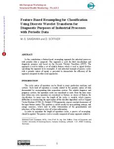
2. DISCRETE WAVELET AND WAVELET PACKET TRANSFORMS 2.1 The Hyperspectral Discrete Wavelet Transform (HSDWT) In the HSDWT1-3, the two-dimensional wavelet transform for the spatial dimensions is independent of the onedimensional DWT in the (third) spectral direction. The (m, n) configuration of the HSDWT consists of an m-level 2D decomposition in the spatial direction, and an n-level decomposition in the spectral direction (see Figure 1).
(a)
(c)
(b)
Y
λ X
Figure 1. Some diagrammatic examples of subband configurations in a HSDWT transformed hyperspectral datacube1,2. (a) HSDWT(3,3), (b) HSDWT(0,3), (c) HSDWT(3,0).
2.2 Wavelet Packet Transforms Wavelet transforms can be generalized for what are known as wavelet packet transforms7. To understand this, it is helpful to review the standard 1D discrete wavelet transform (DWT). Consider Figure 2 which diagrams the standard pyramid algorithm for the one-dimensional wavelet transform. The decomposition lowpass and highpass filters are H and G respectively. Downsampling by a factor of 2 is denoted by an arrow pointing down in Figure 2. The subband notation Wn,s stands for ‘nth level, sth subband,’ and is more general. For a n level wavelet transform, the subbands that are saved are d1, through dn, and an. These correspond to W1,1, W2,1, … Wn,1 and Wn,0 respectively. Note that in the notation Wn,s, s=0 correponds to filtering with the lowpass filter H and s=1 with filtering with the highpass filter G. Wavelet packets result from generalizing this filtering sequence over all such possible subbands, as illustrated in Figure 3. There are many possible filtering tree sequences, but this particular type of sequence is called an ‘equal-subband’ wavelet packet decomposition; here the value of the Wn,s notation for the wavelet packet subbands is evident. There is a procedure called the ‘best-basis’ wavelet packet transform that finds the best tree configuration that maximizes (or minimizes) some sort of cost function at each node of the tree, but that will not be considered here as it is more pertinent to data compression, which is not being done here7. In one dimension, for each level of decomposition n there is 2n subbands, as opposed to n+1 subbands for the DWT. Formally, the filtering procedure in standard wavelet transform (Figure 2) can be represented by the pair of equations
φ ( x) = 2 ∑ h[k ]φ (2 x − k ) k
ψ ( x) = 2 ∑ g[k ]φ (2 x − k ) k
Proc. of SPIE Vol. 6315 63150G-2
(1)
where φ(x) and ψ(x) are the wavelet and scaling functions represented by the filter bank (H, G) given by the filter coefficients h[k] and g[k] respectively; the downsampling by a factor of two is gleaned by inspection. For wavelet packets, let W0(x) = φ(x), and W1(x) = ψ(x), then
W2 n ( x) = 2 ∑ h[k ]Wn (2 x − k ) k
(2)
W2 n +1 ( x) = 2 ∑ g[k ]Wn (2 x − k ) k
represents the process as illustrated in Figure 3.
G 2
d1=W1,1
f(x)
G 2
H
d2=W2,1
a1=W1,0
2
G 2 H 2
d3=W3,1
a2=W2,0 H
2
a3=W3,0
Figure 2. A diagram of the one-dimensional DWT with three levels of decomposition.
G 2 G 2 G 2
W2,3
W1,1
2
G 2
H
f(x)
H
2
W2,2
H 2 G 2
G 2
H
2
W2,1
W1,0
H
2
G 2 H 2
W2,0
H 2
W3,7 W3,6 W3,5 W3,4 W3,3 W3,2 W3,1 W3,0
Figure 3. A. diagram of the equal subband forward wavelet packet transform
If the {H, G} wavelet filter bank is the Haar set (H = 1 / 2 [0.5, 0.5], G = 1 / 2 [0.5, -0.5]), then the equal subband wavelet packet decomposition in Figure 3 is equivalent to the Walsh transform. For reasons of operating simplicity, lack of reconstruction artifacts, and the intent of eventual low-power operations on airborne or spaceborne systems the version of the three dimensional DWT used for hyperspectral signal feature extraction, the HSDWT as described earlier uses a two-dimensional Haar transform in the spatial direction, and a Haar decomposition in the spectral direction2,3.
Proc. of SPIE Vol. 6315 63150G-3
This paper introduces a new variation of the HSDWT replaces the 1D Haar wavelet transform with the 1D Haar / Walsh wavelet packet decomposition in the spectral direction.
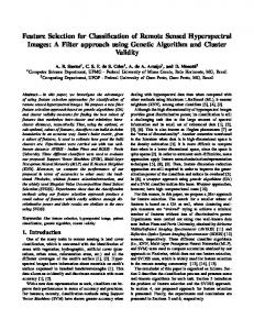
2.3 The Hyperspectral Wavelet – Walsh Transform (HSWWT) This variation of the three-dimensional multiresolution algorithm simply consists of the two-dimensional wavelet transform in the spatial dimensions and the Haar wavelet packet / Walsh transform independently in the spectral direction. As with the HSDWT, the (m, n) configuration of the HSWWT means that the spatial directions have been decomposed with m levels of a 2D DWT, but that in the spatial direction there are n levels of decomposition with the Walsh transform. The HSWWT can either be implemented in a traditional floating-point way, or modified to work on 8or 16-bit integers in a lifting implementation3-6. Figure 4 shows the three-dimensional subband structure of the HSWWT. Note that the (m,0) and (m,1) configurations of the HSWWT are identical with the HSDWT.
Y
λ X
Figure 4. Some diagrammatic examples of subband configurations in a HSWWT transformed hyperspectral datacube1,2. (a) HSWWT(3,1), (b) HSWWT(3,2), (c) HSWWT(3,3). The HSWWT(3,0) and HSWWT(3,1) configurations are identical with HSDWT(3,0) and HSDWT(3,1) respectively.
3. CLASSIFICATION ALGORITHMS 3.1 Generic Classification The generic classification algorithm used in this paper is a special case of linear spectral unmixing. Linear spectral unmixing is a decomposition (or fitting) of the spectrum of an object in a hyperspectral domain with respect to a number of spectra for various features and objects applicable to the task at hand. Consider a hyperspectral datacube with M x N x L voxels; this is a collection of L images of M x N pixels indexed by wavelength band. Additionally, consider a collection of K spectral signatures representing possible features that each pixel could represent. Of course, let the length of each of the K signatures be of length L; the wavelengths in the signatures represent the L bands in the datacube. We then construct a L x K matrix H, where each spectral signature in the collection is a column. If we denote the spectrum of pixel (m,n) in D as the (known) vector x (here [x]l = Dmnl, m-1 to M, n=1 to N, l=1 to L) and the (unknown) vector y = [y]k, k=1 to K as representing the k fractional abundances of the K spectra in pixel x, then x = Hy. In general x and y are not the same length, so H cannot be inverted as it is rectangular. Hence we solve for an estimate of y, denoted by y’ using either a least squares pseudo-inverse H+ = (HtH)-1 Ht, where the superscript t represents the matrix transpose, or a singular value decomposition (SVD) based one. However, the SVD is preferred as it is more numerically stable than least-squares for large systems. In any case, we get y’ = H+x. A potential problem is that some of the
Proc. of SPIE Vol. 6315 63150G-4
weights or abundances in y’ may be negative. These negative weights in this problem are unphysical, so they are set to zero. Linear spectral unmixing becomes classification once the spatial pixel region, field of view or region of interest (ROI) is small enough so that the spectral signature over the spectral directions comes from only one material; that is the abundance percentage is nearly or exactly 100% for a particular material and nearly or exactly 0% for the others. The SVD based linear spectral unmixing procedure just described is unchanged; y’ only has one non-zero component of length unity corresponding to the spectral library signature match. In looking for a feature, this procedure is applied to each and every single (spatial) pixel. For example if we have an AVIRIS datacube set of size (640 x 512 pixels by 224 bands) such a procedure puts enormous stress on computational resources, especially on spaceborne systems, not to mention the demands on power. To alleviate some of these issues redundancies in the data must be exploited, and with efficient auxiliary algorithms. This is where multiresolution data transforms such as wavelets are vital.
3.2 Classification with Wavelet Low-Pass Coefficients The matrix H containing the spectral signatures to fit the pixel’s own spectral signatures is modified in the following fashion2: • The spectral signatures in each column of H are replaced with the lowpass HSDWT transform coefficients in the spectral direction for n levels of decomposition in a (m, n) type HSDWT, as required. • The spectral information over each spatial lowpass transform coefficient in the transformed datacube, also of length L / 2n becomes the data vector x. This • If the lifting algorithm is used in the implementation of the HSDWT, the spectral values in H are discretized to the same number of bits B as the datacube values; that is to a range of values from 0 to 2B-1. In this paper B = 16 to reflect current imaging technology. The advantage of replacing generic classification data with the corresponding lowpass wavelet transform coefficients is faster calculation using less memory. However this will be negated by the fact that as the number of spectral levels of decomposition n increases, the datacube and library signatures in H will all smooth out (as a lowpass filter will do) and appear increasingly similar to each other. Then the generic spectral unmixing algorithm will break down. In this paper we consider two alternatives.
3.3 Classification with Wavelet High-Pass Coefficients In this configuration each column of H which represents a library spectral signature is replaced by its corresponding wavelet transform coefficient set denoted as d1 or W1,1 as in Figure 2, which contains the highest spatial frequency information in that signal. How well that replacement will work instead of the original spectral signatures will depend on how different they are from each other as measured by the (SVD) condition number of H as discussed in detail in Section 5.
3.4 Classification Using Walsh Functions In this configuration each column of H which represents a library spectral signature is replaced by its corresponding equal subband Haar wavelet packet (or Walsh) transform coefficient set denoted as Wn,s as in Figure 3. Here the subscript “n, s” represents the nth level of decomposition, and subband s in that level where s = 0 to 2n-1. This contains more arbitrary spatial frequency information of that signal. How well that replacement will work instead of the original spectral signatures will also depend on how different they are from each other as measured by the (SVD) condition number of H as discussed in detail in Section 5.
Proc. of SPIE Vol. 6315 63150G-5
4. TEST DATA 4.1 The Test Image and Spectral Library For this paper we examined a simulated hyperspectral datacube image of the Hubble Space Telescope (Figure 5). This image was 256 x 256 pixels, with each pixel in the object having a reflectance spectral signature of length 155 from 351 to 1891 nm in steps of 10 nm. Thus the wavelength range of the data is from the visible to the shortwave-infrared (SWIR). The spacecraft was comprised of only four material spectra (Figure 7) used in the simulation: aluminum, mylar, solar cells, and white paint, as illustrated in Figures 6a-e. Data such as in Figures 5, 6 and 7 would typically be used for a computational testbed as described in earlier papers3,8. Actual implementation of this enables tasks such as spectral library manipulation, adding noise and other image degradation, wavelet transforms, and feature extraction algorithms.
Figure 5. The PSF blurred simulated image of the Hubble Space Telescope (HST) at λ=500 nm .
(b)
(a)
(e)
Aluminum
(c)
Mylar
(d)
Solar cell
White Paint
Figure 6. The spectral ground truth for the HST object. Pictures (a)-(d) assign the respective material spectral signatures to the indicated pixels. Picture (e) represents the correct pixel material classifications corresponding to (a)-(d).
Proc. of SPIE Vol. 6315 63150G-6
Mean - Mylar
Mean - Aluminum 90
90
80
80
70
70
Reflectance
100
Reflectance
100
60 50 40 30
60 50 40 30
20
20
10
10 0
0 0
0.5
1
Wavelength (µm)
1.5
0
2
0.5
Mean - Solar Cell 90
90
80
80
70
70
Reflectance
100
Reflectance
100
60 50 40 30 20
1
1.5
2
1.5
2
Wavelength (µm)
Mean - White Paint
60 50 40 30 20
10
10
0 0
0.5
1
1.5
0
2
0
Wavelength (µm)
0.5
1
Wavelength (µm)
Figure 7. The spectral signature library used for the calculations in this paper, courtesy of Maile Giffin at Oceanit Laboratories, Inc.
5. CALCULATIONS 5.1 Condition Number Calculations By inspection of the spectral signature library there were spectral sub-ranges where the signatures were very similar to each other, and others where the signatures were least similar to each other. We then computed an optimal spectral subrange before any wavelet transform was done. This was chosen by sliding windows from 80 to 154 spectral bins in length over the visible to SWIR range, and for each case, the SVD condition number for the unmixing matrix H was computed. A higher number indicates the signatures are more similar to each other, which makes feature algorithms more difficult to work. The position and length of the spectral sub-range was chosen that minimizes this condition number. The range between 351 and 1541 nm was found to have the lowest SVD condition number. With a 10 nm spectral binwidth this corresponded to 120 wavelength samples; this number was adopted rather than 116 since the former number is amenable to wavelet transforms for three levels of decomposition instead of two. This is illustrated in Figures 8a-b 250
120
Start of Window r 351 nm 110
n
a)
E
Z 100 C 0 90
0 80
(a)
Window Length 120 80
100
120
140
Spectral Signature Length
160
(b)
400 450 500 550 600 650 700 750 Starting Wavelength (nm)
Figure 8. (a) Finding best window length in spectral direction; (b) Finding best starting wavelength of window.
Proc. of SPIE Vol. 6315 63150G-7
The next step was to do 1D wavelet or wavelet packet transforms on the library spectral signatures in that 120 length sample range and compute the condition number for the SVD decomposition of the corresponding H matrix, for no wavelet transforms, for the lowpass wavelet transform coefficient for three levels of decomposition, the highest frequency highpass wavelet coefficients, and for the particular wavelet packet transform subband with the best value. These results are summarized in Table 1. Table 1 SVD Condition Numbers for H Type of Wavelet Decomposition SVD Condition Number for Corresponding H None 74.85 DWT 3 Levels, Lowpass - W3,0 (a3) subband 183.98 DWT 3 Levels, Highpass – W1,1 (d1) subband 9.59 Wavelet Packet / Walsh 3 Levels, W3,6 subband 4.75
5.2 Classification Calculations Classification calculations were done with each of the four wavelet / wavelet packet configurations in Table 1 on the simulated hyperspectral HST imagery for the following cases: 1) the satellite data with no blurring or pixel noise, 2) data with typical spatio-temporal pixel noise that would be seen through a large ground based telescope; the pixel noise represents that which is “frozen” at the moment of data capture, and 3) the simulated satellite image with only spatial / spectral blur of the form
PSF(r, λ) =
a(λ ) =
1 ⎛ ⎛ r ⎞2 ⎞ ⎜1 + ⎜ ⎟ ⎟ ⎜ ⎜⎝ a(λ ) ⎟⎠ ⎟ ⎝ ⎠
3 21/3
3
⎛ λ ⎞ ⎜ ⎟ − 1 ⎝ 0.5 ⎠
(3) −1/5
where the length units are in pixels, and the wavelength is in microns. The confusion matrices are presented in Tables 2-10. The results are summarized in Table 11. Table 2 Object confusion matrix, all wavelet / wavelet packet configurations No blurring or pixel noise Predicted Pixel Classification Actual material Actual Pixel spectra Totals 1 2 3 4 in each pixel Aluminum 494 0 0 0 1 494 Mylar 0 1317 0 0 2 1317 Solar Cell 0 0 959 0 3 959 White Paint 0 0 0 177 4 177 Predicted Totals 494 1317 959 177 2947
Proc. of SPIE Vol. 6315 63150G-8
Actual material spectra in each pixel Aluminum 1 Mylar 2 Solar Cell 3 White Paint 4 Predicted Totals
Actual material spectra in each pixel Aluminum 1 Mylar 2 Solar Cell 3 White Paint 4 Predicted Totals
Table 3 Object confusion matrix, no wavelet transform Pixel noise only Predicted Pixel Classification 1 2 3 4 494 0 0 0 494
0 1317 0 0 1317
0 0 959 0 959
0 0 0 177 177
Table 4 Object confusion matrix, no wavelet transform PSF blurring only Predicted Pixel Classification 1 2 3 4 0 0 0 0 0
494 1317 959 130 2900
0 0 0 0 0
0 0 0 47 47
Actual Pixel Totals 494 1317 959 177 2947
Actual Pixel Totals 494 1317 959 177 2947
Table 5 Object confusion matrix, wavelet transform – lowpass (W3, 0 or a3) coefficients Pixel noise only Predicted Pixel Classification Actual material Actual Pixel spectra Totals 1 2 3 4 in each pixel Aluminum 494 0 0 0 1 494 Mylar 0 1317 0 0 2 1317 Solar Cell 0 0 959 0 3 959 White Paint 0 0 0 177 4 177 Predicted Totals 494 1317 959 177 2947 Table 6 Object confusion matrix, wavelet transform – lowpass (W3,0 or a3) coefficients PSF blurring only Predicted Pixel Classification Actual material Actual Pixel spectra Totals 1 2 3 4 in each pixel Aluminum 0 494 0 0 1 494 Mylar 0 1317 0 0 2 1317 Solar Cell 0 959 0 0 3 959 White Paint 0 123 0 54 4 177 Predicted Totals 0 2893 0 54 2947
Proc. of SPIE Vol. 6315 63150G-9
Table 7 Object confusion matrix, wavelet transform – highpass (W1,1 or d1) coefficients Pixel noise only Predicted Pixel Classification Actual material Actual Pixel spectra Totals 1 2 3 4 in each pixel Aluminum 493 0 1 0 1 494 Mylar 0 1315 2 0 2 1317 Solar Cell 0 0 959 0 3 959 White Paint 0 0 0 177 4 177 Predicted Totals 493 1315 962 177 2947
Table 8 Object confusion matrix, wavelet transform – highpass (W1,1 or d1) coefficients PSF blurring only Predicted Pixel Classification Actual material Actual Pixel spectra Totals 1 2 3 4 in each pixel Aluminum 0 7 485 2 1 494 Mylar 0 1087 175 55 2 1317 Solar Cell 0 0 959 0 3 959 White Paint 0 0 34 143 4 177 Predicted Totals 0 1094 1653 200 2947 Table 9 Object confusion matrix, wavelet packet / Walsh transform – W3,6 subband Pixel noise only Predicted Pixel Classification Actual material Actual Pixel spectra Totals 1 2 3 4 in each pixel Aluminum 249 24 152 69 1 494 Mylar 0 1290 23 4 2 1317 Solar Cell 23 29 762 145 3 959 White Paint 1 0 32 144 4 177 Predicted Totals 273 1343 969 362 2947 Table 10 Object confusion matrix, wavelet packet / Walsh transform – W3,6 subband PSF blurring only Predicted Pixel Classification Actual material Actual Pixel spectra Totals 1 2 3 4 in each pixel Aluminum 398 30 66 0 1 494 Mylar 0 1255 62 0 2 1317 Solar Cell 592 38 329 0 3 959 White Paint 0 17 160 0 4 177 Predicted Totals 990 1340 617 0 2947
Proc. of SPIE Vol. 6315 63150G-10
Type of Image Degradation
No Noise or Blurring Pixel Noise Only PSF Blurring Only
Table 11 Percent of Correct Classification No Wavelet Wavelet Wavelet Transform Transform Transform Lowpass Highpass (W3,0 or a3) (W1,1 or d1) Coefficients Coefficients 100.0 100.0 100.0 100.0 100.0 99.9 45.9 46.0 74.3
Wavelet Packet/Walsh Transform W3,6 Subband Coefficients 100.0 83.0 67.3
5.3 Discussion The improvement in classification the datacube with PSF blurring generally follows the SVD condition number for the H matrices with the corresponding library spectral signature wavelet transform configurations given in Table 1. This confirms the intuition and the use of the condition number in this analysis. Wavelet and wavelet packet transform coefficients which contain higher spatial / spectral frequency information differentiates or ‘separates’ each library signature from each other. However in the case where there is pixel noise, wavelet or wavelet packet transforms that contain higher spatial / spectral frequency information accentuate this noise. This results in a decrease in classification efficiency using the W1,1 and W3,6 coefficient sets.
6. CONCLUSIONS We have implemented the use of higher frequency wavelet transform coefficients and the more general wavelet packet transforms in the spectral domain for classification (and by extension linear spectral unmixing) algorithms. These more general sets of wavelet coefficients emphasize the differences between the library spectral signatures and therefore improve pixel-by-pixel classification for hyperspectral datacubes where there has been blurring. In addition the use of the SVD condition number of H constructed with a particular wavelet / wavelet packet transform of the library spectra appears to be quite useful as a figure-of-merit for evaluating library signature separability. This was initially examined in an earlier paper8. However there is a tradeoff to be made for pixel noise. Classification using wavelet packet transform coefficients in narrow, high spatial / spectral frequency bands decreases in effectiveness for datacubes with pixel noise as this noise is accentuated. It appears then, that particular sets of wavelet packet transform coefficients are useful in hyperspectral datacubes with particular types of image degradations or other types of characteristics (such as spectral signature variations within each class); this needs to be investigated further. Another issue that needs to be explored is the range of applicability of the SVD based figure-of-merit in the presence of data with more complicated features as the intra-class spectra variations just mentioned. These issues are discussed in more detail in a follow-up paper9 also in this same conference proceedings volume.
Proc. of SPIE Vol. 6315 63150G-11
REFERENCES 1. J. F. Scholl and E. L. Dereniak, “Higher-dimensional wavelet transforms for hyperspectral data compression and feature recognition,” Proceedings of SPIE, Volume 5208: Mathematics of Data/Image Coding, Compression and Encryption VI with Applications, M. S. Schmalz, editor, pp. 129-140, (2003). 2. J. F. Scholl and E. L. Dereniak, “Fast wavelet based feature extraction of spatial and spectral information from hyperspectral datacubes,” Proceedings of SPIE, Volume 5546: Imaging Spectrometry X, S. S. Shen and P. E. Lewis, editors, pp. 285-293, (2004). 3. J. F. Scholl, E. L. Dereniak and E. K. Hege, “Fast feature extraction in hyperspectral imagery using lifting wavelet transforms,” Proceedings of SPIE, Volume 5915: Mathematics of Data/Image Coding, Compression and Encryption VIII with Applications, M. S. Schmalz, editor, pp. 59150N 1-12, (2005). 4. D. S. Taubman and M. W. Marcellin, JPEG2000: Image Compression Fundamentals, Standards and Practice, (Boston MA: Kluwer Academic Publishers), 2002. 5. W. Sweldens, “The lifting scheme: A custom-design construction of biorthogonal wavelets,” Applied and Computational Harmonic Analysis, 3, 186-200, (1996). 6. R. Calderbank, I. Daubechies, W. Sweldens and B. Yeo, “Wavelet transforms that map integers to integers,” Applied and Computational Harmonic Analysis, 5, 332-369, (1998). 7. S. Mallat, A Wavelet Tour of Signal Processing, second edition, (Academic Press), 1999, Chapter VIII. 8. J. F. Scholl, E. K. Hege, M. Lloyd-Hart, D. O’Connell, W. R. Johnson, and E. L. Dereniak, “Evaluations of classification and spectral unmixing algorithms using ground based satellite imaging,” Proceedings of SPIE, Volume 6233: Algorithms and Technologies for Multispectral, Hyperspectral, and Ultraspectral Imagery XII, S. S. Shen and P. E. Lewis, editors, to be published, (2006). 9. J. F. Scholl, E. K. Hege and E. L. Dereniak, “Figure of merit calculations for spectral unmixing and classification algorithms,” Proceedings of SPIE, Volume 6315: Mathematics of Data/Image Pattern Recognition, Compression and Encryption with Applications, G. X. Ritter, M. S. Schmalz, J. Barrera and J. T. Astola, editors, to be published, 2006.
Proc. of SPIE Vol. 6315 63150G-12