One of the earliest data association algorithms was the track splitting filter [1], also .... The Probabilistic Data Association (PDA) Filter, sometimes referred to as a â ...
ADDRESSING TRACK COALESCENCE IN SEQUENTIAL K-BEST MULTIPLE HYPOTHESIS TRACKING
A Thesis Presented to The Academic Faculty By Ryan D. Palkki
In Partial Fulfillment of the Requirements for the Degree Master of Science in Electrical and Computer Engineering
School of Electrical and Computer Engineering Georgia Institute of Technology August 2006
ADDRESSING TRACK COALESCENCE IN SEQUENTIAL K-BEST MULTIPLE HYPOTHESIS TRACKING
Approved by:
Dr. Aaron Lanterman, Advisor School of Electrical and Computer Engineering Georgia Institute of Technology
Dr. James McClellan School of Electrical and Computer Engineering Georgia Institute of Technology
Dr. Magnus Egerstedt School of Electrical and Computer Engineering Georgia Institute of Technology
Date Approved: May 10, 2006
To my beautiful wife, Brenna.
ACKNOWLEDGMENTS I wish to thank my advisor, Aaron Lanterman, for his ongoing guidance over this work. I also wish to thank Dale Blair for his support and suggestions throughout the course of this research. Finally, I wish to thank the other members of my group for all the time and help that they are always willing to give. This work was funded by U.S. Office of Naval Research grant N00014-04-C-0406.
iv
TABLE OF CONTENTS ACKNOWLEDGMENTS . . . . . . . . . . . . . . . . . . . . . . . . . . . . . . .
iv
LIST OF TABLES . . . . . . . . . . . . . . . . . . . . . . . . . . . . . . . . . . . vii LIST OF FIGURES . . . . . . . . . . . . . . . . . . . . . . . . . . . . . . . . . . viii SUMMARY . . . . . . . . . . . . . . . . . . . . . . . . . . . . . . . . . . . . . .
ix
CHAPTER 1 INTRODUCTION . . . . . . . . . . . . . . . . . . . . . . . . . . 1.1 The Data Association Problem . . . . . . . . . . . . . . . . . . . . . . . 1.2 Nearest Neighbor and Track Splitting Filters . . . . . . . . . . . . . . . . 1.3 The Optimal Filter and the Criteria for the Estimator . . . . . . . . . . . . 1.3.1 “Hard” (MAP) vs. “Soft” (MMSE) Association . . . . . . . . . . 1.4 Approximations to the Optimal Filter . . . . . . . . . . . . . . . . . . . . 1.4.1 The PDA and N-Scan Approximations to the Optimal MMSE Filter 1.4.2 Sequential K-Best MHT . . . . . . . . . . . . . . . . . . . . . . 1.5 Outline of the Rest of the Thesis . . . . . . . . . . . . . . . . . . . . . .
1 1 1 2 2 3 4 5 8
CHAPTER 2 SIMULATION FRAMEWORK . . . . . . 2.1 Assumptions and Filter Model . . . . . . . . . . . . 2.2 Track Score Function . . . . . . . . . . . . . . . . 2.3 Reasonability of the MAP estimate for K-Best MHT 2.4 Performance Metrics . . . . . . . . . . . . . . . . . 2.5 Truth Trajectory, False Alarms, and Gating . . . . . 2.6 Process Noise Tuning . . . . . . . . . . . . . . . . CHAPTER 3
. . . . . . .
. . . . . . .
. . . . . . .
. . . . . . .
. . . . . . .
. . . . . . .
. . . . . . .
. . . . . . .
. . . . . . .
. . . . . . .
. . . . . . .
9 9 10 11 12 13 14
COMPARING K-BEST MHT WITH PDA . . . . . . . . . . . . 18
CHAPTER 4 DEALING WITH TRACK COALESCENCE 4.1 The Simple “Measurement Constraint” Method . . . 4.2 Tighter Coalescence Tests . . . . . . . . . . . . . . . 4.2.1 Tighter Test I . . . . . . . . . . . . . . . . . 4.2.2 Tighter Test II . . . . . . . . . . . . . . . . . 4.3 Looser Coalescence Tests . . . . . . . . . . . . . . . 4.4 The J-Divergence Test . . . . . . . . . . . . . . . . . CHAPTER 5
. . . . . . .
. . . . . . .
. . . . . . .
. . . . . . .
. . . . . . .
. . . . . . .
. . . . . . .
. . . . . . .
. . . . . . .
. . . . . . .
. . . . . . .
. . . . . . .
20 20 21 21 22 24 26
CONCLUSION . . . . . . . . . . . . . . . . . . . . . . . . . . . 30
APPENDIX A RESULTS OF “TIGHTER TEST I” OF SECTION 4.2.1 . . . . 31 APPENDIX B RESULTS OF THE MAHALANOBIS TESTS OF SECTION 4.3 32
v
APPENDIX C KULLBACK-LEIBLER DISTANCE FOR MULTIVARIATE GAUSSIAN NORMAL DISTRIBUTIONS . . . . . . . . . . . . . . . . 33 REFERENCES . . . . . . . . . . . . . . . . . . . . . . . . . . . . . . . . . . . . . 36
vi
LIST OF TABLES Table 1
Process noise parameters tested. . . . . . . . . . . . . . . . . . . . . . . 15
Table 2
Which σ2v works best? . . . . . . . . . . . . . . . . . . . . . . . . . . . 16
Table 3
Track loss ratio of PDA. . . . . . . . . . . . . . . . . . . . . . . . . . . 18
Table 4
Track loss ratio of K-Best MHT (with measurement constraint to prevent track coalescence). . . . . . . . . . . . . . . . . . . . . . . . . . . . . . 18
Table 5
The bottom left corner of Table 4, but now with 10,000 Monte Carlo Runs. 19
Table 6
Track loss ratio of K-Best MHT without any method to prevent track coalescence; compare with Table 4. . . . . . . . . . . . . . . . . . . . . 21
Table 7
Track loss ratio of K-Best MHT with the J-Divergence Test. . . . . . . . 29
Table 8
Track loss ratio of K-Best MHT when the threshold is 2. . . . . . . . . . 31
Table 9
Track loss ratio of K-Best MHT when the threshold is 3. . . . . . . . . . 31
Table 10
Track loss ratio of K-Best MHT when the threshold is 4. . . . . . . . . . 31
Table 11
Track loss ratio of K-Best MHT when d12 is used as the Mahalanobis distance. . . . . . . . . . . . . . . . . . . . . . . . . . . . . . . . . . . 32
Table 12
Track loss ratio of K-Best MHT when d22 is used as the Mahalanobis distance. . . . . . . . . . . . . . . . . . . . . . . . . . . . . . . . . . . 32
Table 13
Track loss ratio of K-Best MHT when d32 is used as the Mahalanobis distance. . . . . . . . . . . . . . . . . . . . . . . . . . . . . . . . . . . 32
vii
LIST OF FIGURES Figure 1
Flowcharts of the NN and K-Best Trackers. . . . . . . . . . . . . . . . .
6
Figure 2
Results after each of the six steps of the K-Best algorithm as numbered in the flowchart of Figure 1(b). In this example, K = 2, and we happen to also have two measurements. For simplicity, gating is not shown, and the missed-detection hypotheses are not considered (both of these steps are straightforward). L is the cumulative track score, ∆ L is the incremental score, ‘ +’ denotes a track prediction, ‘ *’ represents a measurement, and the connecting lines are the possible data associations. The stars are filtered estimates, and the filled star is the output track state estimate of the K-Best tracker. . . . . . . . . . . . . . . . . . . . . . . . . . . . . .
7
Illustration of the Sequential K-Best MHT tracker. Target is moving from right to left. . . . . . . . . . . . . . . . . . . . . . . . . . . . . . .
8
Figure 3 Figure 4
Truth trajectory and measurements of a simulation. Target is moving from right to left. . . . . . . . . . . . . . . . . . . . . . . . . . . . . . . 14
Figure 5
Histogram of the results presented in Table 2. The height of the graph at any of the seven process noises is the number of tracking scenarios for which that process noise was preferred over all of the others. . . . . . . . 17
Figure 6
Track loss ratio for the PD = 0.94, βFA = 0.04 case. . . . . . . . . . . . . 19
Figure 7
Illustration of track coalescence when K = 3. Target is moving from right to left. . . . . . . . . . . . . . . . . . . . . . . . . . . . . . . . . . 20
Figure 8
Track loss ratio when PD = .94, βFA = .04. . . . . . . . . . . . . . . . . 23
Figure 9
Track loss ratio when PD = .94, βFA = .04. . . . . . . . . . . . . . . . . 24
Figure 10 Track loss ratio when PD = .94, βFA = .04. . . . . . . . . . . . . . . . . 26 Figure 11 Even if two tracks are close together, they are likely to pick different measurements if the covariances are different. . . . . . . . . . . . . . . . 27 Figure 12 Track loss ratio when PD = .94, βFA = .04. . . . . . . . . . . . . . . . . 29
viii
SUMMARY Multiple Hypothesis Tracking (MHT) is generally the preferred data association technique for tracking targets in clutter and with missed detections due to its increased accuracy over conventional single-scan techniques such as Nearest Neighbor (NN) and Probabilistic Data Association (PDA). However, this improved accuracy comes at the price of greater complexity. Sequential K-best MHT is a simple implementation of MHT that attempts to achieve the accuracy of multiple hypothesis tracking with some of the simplicity of single-frame methods. Our first major objective is to determine under what general conditions Sequential Kbest data association is preferable to Probabilistic Data Association. Both methods are implemented for a single-target, single-sensor scenario in two spatial dimensions. Using the track loss ratio as our primary performance metric, we compare the two methods under varying false alarm densities and missed-detection probabilities. Upon implementing a single-target Sequential K-best MHT tracker, a fundamental problem was observed in which the tracks coalesce. The second major thrust of this research is to compare different approaches to resolve this issue. Several methods to detect track coalescence, mostly based on the Mahalanobis and Kullback-Leibler distances, are presented and compared.
ix
CHAPTER 1 INTRODUCTION 1.1 The Data Association Problem Assuming that a good linear dynamics model for a target of interest is available, along with a sequence of measurements that are linearly related to the target state and that are corrupted by Gaussian noise, the target tracking problem is well solved by the Kalman Filter. The Kalman Filter is the optimal recursive data processing filter in such cases.1 However, the classic Kalman Filter equations do not take into account any uncertainty in the origins of the measurements; they assume we know that the measurement received on each scan originated from the target of interest [1]. The Kalman Filter deals optimally with measurement error, but it does not deal at all with measurement-origin uncertainty. In a realistic tracking scenario, there will be measurements originating from other targets or from clutter (false alarms), and sometimes no measurement will be received at all even though the target of interest was there (missed detections). The Kalman update equation may then use the wrong measurement to update the track estimate, and the tracker performance may be severely degraded. For this reason, the problem of “data association,” i.e., the problem of deciding which—if any—measurement originated from which target, has historically been one of the greatest problems in target tracking.
1.2 Nearest Neighbor and Track Splitting Filters The simplest method of data association is the Nearest Neighbor filter. This method finds the measurement from the current scan that is statistically closest to the track prediction. It then uses this “nearest neighbor” in the Kalman Filter update equation, while ignoring all of the other measurements from that scan. Since this method may ignore some of the observed data, it is reasonable that better data association algorithms should be possible. 1
If the dynamics model and/or the measurement model are nonlinear, an Extended Kalman Filter (EKF) may be employed. The EKF algorithm is suboptimal, but it is effective in many applications.
1
One of the earliest data association algorithms was the track splitting filter [1], also called the branching algorithm [2], which simply splits the track whenever multiple measurements fall within the validation (gating) region2 of the track prediction. The number of branches of the track can grow exponentially with time, and it becomes necessary to “prune” (eliminate) the tracks whose likelihood is below a threshold. The number of tracks (and the memory requirements) still grow with time, despite this pruning.
1.3 The Optimal Filter and the Criteria for the Estimator Understanding the track splitting filter helps in thinking about the general problem of data association. If the track splitting filter were to run for k scans, and there was no pruning of unlikely tracks, then there would be a large number of possible tracks by the time that scan k is received (if M is the number of possible tracks, then M grows exponentially with k). Each of those M tracks has a certain probability of being the true track. For any individual track j among those M possible tracks, given that track j is the true track, the posterior pdf of the target state would be Gaussian. Since it is not known which of the M branches is the true target track, the posterior pdf of the target state given all of the measurements from all of the scans will be a probabilistically weighted mixture of Gaussians. It is theoretically possible to keep track of all of the possible tracks (i.e., to not prune any of the branches, no matter how unlikely) and to compute the probability of each one. It is thus also possible, at least in theory, to compute the Gaussian mixture posterior distribution of the target state given all received measurements over the entire history of scans through scan k. 1.3.1
“Hard” (MAP) vs. “Soft” (MMSE) Association
Once the posterior distribution of the target state is found, one can take its mean to find the minimum-mean-squared-error (MMSE) estimate of the target state. This is a “soft 2
To reduce computational requirements, any measurements that fall outside of a “gate” region centered around the track prediction are not considered in the data association problem.
2
association” approach; the estimate used for the track update does not correspond to one particular measurement, but rather results from a weighted combination of data associations from all of the possible measurements. Although this estimate is optimal in the MMSE sense, there are situations in which it is desirable to make a hard decision rather than a soft decision. As Drummond [3] points out, “for estimation involving hypotheses due to discrete possibilities, the traditional MMSE criterion leads to so called soft decisions that may not be appropriate for an interceptor with a small region of lethality while, in contrast, hard decisions might increase the probability of kill.” For this reason, the maximum a posteriori (MAP) estimate, which finds the state that maximizes the posterior distribution, may be preferred. Most Multiple Hypothesis Tracking (MHT) methods are essentially MAP estimators [4]. In section 2.3, we show that a hard (MAP) association approach appears to be reasonable for our Sequential K-Best MHT.
1.4 Approximations to the Optimal Filter The optimal3 Bayesian (MMSE) approach described above was implemented for a simple scenario by Singer et al. [5] in 1974. The major problem with this method (as well as any method that employs no scheme to prune and manage the number of tracks, including the optimal MAP method) is that it is practically infeasible for realistic scenarios. As mentioned previously, the number of branches grows exponentially with time. So, instead of implementing the full-blown optimal algorithm, most classical tracking methods aim for one of the optimal criteria (MMSE or MAP, or something else, like maximum likelihood (ML)), but impose some approximations to make the algorithm feasible. For example, the track splitting filter becomes feasible when the unlikely branches are eliminated. Here, the approximation made to the optimal filter is done by representing all of the possible 3
The approach is “optimal” among methods that assume that multiple measurements will not originate from a single target; so far, we have made this common assumption. If there is one track and N measurements PN �N � = 2N association hypotheses down to N + 1 hypotheses under consideration, this constraint cuts the n=0 n per scan. After M scans, there will be (N + 1) M tracks, compared to (2N ) M . While the number of branches still grows exponentially with the number of scans, it grows at a much slower rate. In comparison, the single-target K-Best MHT maintains a constant number of tracks and the load remains fixed.
3
branches by a subset of the most likely branches. With this approximation, it is feasible to compute an approximate posterior distribution. If the goal is to minimize MMSE, then a soft association will be used to obtain the track state estimate from the (approximate) posterior distribution. If a MAP or ML criterion is used, then a hard association will be made according to that criterion. 1.4.1
The PDA and N-Scan Approximations to the Optimal MMSE Filter
The Probabilistic Data Association (PDA) Filter, sometimes referred to as a “suboptimal Bayesian approach,” is another example of a suboptimal algorithm. PDA4 seeks to minimize MMSE; hence, it is a soft association approach. It makes a major approximation to the optimal MMSE filter: whereas the posterior density of the state given all past observations is really a Gaussian mixture, the PDAF approximates this density with a single Gaussian with the same mean and variance [6]. Using PDA, only one track is propagated forward at each scan (instead of an exponentially increasing number of tracks), and the computational requirements do not increase with time. Because it takes all of the measurements from the current scan into account, it performs better in dense clutter than the NN filter. However, the extra computational burden is small (“about 50% greater” than the NN Filter [6]). When Singer et al. derived and implemented the optimal Bayesian (MMSE) filter [5], they also proposed an approximation to it. Instead of splitting the track all the way back through its history, they split it for only the last N scans. This approximation is equivalent to combining any tracks that have the last N measurements in common. Since this suboptimal version still seeks the MMSE criterion, it uses the soft association approach and recombines the tracks into one mixed estimate. Thus, when N = 0, this so-called Generalized PseudoBayesian filter [4] reduces to the PDA filter. Singer et al. then show that N = 1 and N = 2 gave “near-optimal” results [7]. Note that this N-scan method requires a history, i.e. “window,” of data if N > 0. Improved performance comes with the cost of greater 4
The Joint Probabilistic Data Association (JPDA) method is an extension of PDA to the multiple-target case.
4
complexity. 1.4.2
Sequential K-Best MHT
The above examples illustrate the nature of most classical tracking methods. The theoretically optimal algorithms described previously are infeasible, so approximations are made to make them feasible. This is also the case with the Sequential K-Best Multiple Hypothesis Tracker. The Sequential K-Best MHT is similar to the track-splitting filter, except that it allows only K total tracks to exist at each scan. The K-Best method finds the K best measurementto-track assignments (given by the recursive probability-based score of [8]; see Section 2.2) for each scan of data received. The K hypotheses are ranked from the most likely down to the K th most likely hypothesis. Then, on the next scan, it finds the K best associations from all of the K tracks maintained from the previous scan. At each scan, the track with the highest score is the output track state estimate (see Section 2.3). This process is illustrated and compared with the Nearest Neighbor method in Figure 1. The six steps of the algorithm are illustrated for a simple example in Figure 2. Figure 3 illustrates how the K-best MHT tracker “feels around for” the true trajectory. As shown in the figure, the best track at the current scan is sometimes later shown not to be the best when considered in the light of further data. In this way, Sequential K-Best MHT avoids losing the track as NN would have. Another difference between NN and K-Best MHT is that while the NN filter always updates the track with the nearest measurement, the MHT filter also considers the case that all the measurements may be false alarms, i.e., there is a missed detection. Sometimes, the observations are so far away from the track prediction that it is more likely that all of them are false alarms, and that there was a missed detection of the target, than that one of them represents the target. The MHT filter takes this into account. Thus, even with K = 1, Sequential K-Best MHT will often outperform NN if there are missed detections. Measurement gating is effectively a crude way for NN to approximate the K = 1 MHT—if
5
Propagate K tracks forward ("prediction") 1 Measurements from sensor
Wait to receive new scan of measurements 2
Propagate single track forward ("prediction") Measurements from sensor
Compute incremental scores for all possible measurement-to-track associations on current scan 3
Wait to receive new scan of measurements
Add these to the corresponding cumulative track scores from previous scan to get new cumulative scores
Calculate which measurement is statistically closest to track prediction. Throw out the rest.
4 Rank cumulative scores; keep K best associations 5
Run Kalman Filter to filter single prediction with single measurement ("correction")
Use highest-scoring track as output track state estimate
(a) NN algorithm
Run Kalman Filter on K best measurement-to-track associations ("correction")
6
(b) Sequential K-Best MHT algorithm
Figure 1. Flowcharts of the NN and K-Best Trackers.
a measurement is too far away from the track, the gating causes NN to coast rather than pick the unlikely nearest neighbor.5 Sequential K-Best MHT is similar to PDA in that they are both simple recursive methods that do not require memory of past scans. For this reason, the important performance comparison of this thesis will be Sequential K-Best MHT with PDA. To our knowledge, such a comparison for these single-target trackers has not been documented. 1.4.2.1
Sequential K-Best in the Literature
In multiple target tracking, a common way to keep the number of hypotheses from exploding is to maintain and propagate forward only the K best (often called the “m best”, “M best”, or “N best”) hypotheses from each scan, where a hypothesis is a set of compatible tracks. Cox and Hingorani [9] discovered that Murty’s algorithm [10] can be used to efficiently find the K best solutions to the 2-D assignment problem without using exhaustive enumeration of all of the possible hypotheses. This pruning method is a common way to 5
When a “maximum likelihood gate” [8] is used, NN becomes equivalent to K = 1 MHT.
6
L = 10 R=1
L=7 R=2
(a) Step 1
∆L = 4
∆L = 5
(b) Step 2
L = 14
∆L = 9
∆L = 6
L = 15
(c) Step 3
L = 16
L = 13
(d) Step 4
L = 16 R=1
L = 16
L = 15 R=2
L = 15
(e) Step 5
(f) Step 6
Figure 2. Results after each of the six steps of the K-Best algorithm as numbered in the flowchart of Figure 1(b). In this example, K = 2, and we happen to also have two measurements. For simplicity, gating is not shown, and the missed-detection hypotheses are not considered (both of these steps are straightforward). L is the cumulative track score, ∆ L is the incremental score, ‘ +’ denotes a track prediction, ‘ *’ represents a measurement, and the connecting lines are the possible data associations. The stars are filtered estimates, and the filled star is the output track state estimate of the K-Best tracker.
7
0
−0.5
nearest neighbor truth trajectory
Y (km)
−1
−1.5
track prediction gating (validation) region
−2 2nd best measurement −2.5 89
89.5
90
90.5 X (km)
91
91.5
92
Figure 3. Illustration of the Sequential K-Best MHT tracker. Target is moving from right to left.
implement hypothesis-oriented MHT for the multiple-target scenario. However, we have not seen the K-Best method explored in the single-target scenario, and we have not found any performance comparisons between K-Best MHT and PDA. We have also not seen the issue of track coalescence (see Chapter 4) addressed for single-target K-Best MHT.
1.5 Outline of the Rest of the Thesis First, Chapter 2 explores the simulation framework used by all of our trackers. Some of the key assumptions, decisions, and implementation issues are addressed. Chapter 3 presents the simulation results of K-Best MHT and PDA, and compares the two under different tracking scenarios. Chapter 4 addresses the observed problem of track hypothesis coalescence and compares the results of various methods of detecting coalescence. Finally, a conclusion is presented.
8
CHAPTER 2 SIMULATION FRAMEWORK We incorporated a Sequential K-Best MHT tracker into a MATLAB-based tracking framework developed primarily by Terry Ogle and Dale Blair at the Georgia Tech Research Institute. This chapter outlines the simulation framework and some of the implementation issues that were addressed.
2.1 Assumptions and Filter Model Several points need to made about the scope of this research. All of our trackers operate in two spatial dimensions on single point targets.1 Although measurements are assumed to be corrupted by noise, we neglect the effects of finite sensor resolution. We assume that binary detection decisions have already been made, and no signal-related data (i.e., signal-to-noise ratio) is used. All of these matters are important issues in real-world trackers, and will need to be considered as part of future work. The sensor is assumed to receive range and azimuth measurements. This means the observed output y is a nonlinear function of the Cartesian state x, and a nonlinear estimator is needed. A standard Extended Kalman Filter (EKF) is used, which does not appear to have any problems in this application. We use a Constant Velocity (CV) state model, which models the random target dynamics via a white noise acceleration. In our study, the model is implemented directly in the discrete-time domain and is piecewise-constant between sampling times; this differs from the discretized continuous-time model, which is also sometimes used [8]. 1
The single-target assumption is especially important, as it allows us to delve into the issues of interest without being distracted by issues such as track initiation and deletion. Extending this research to the multiple-target scenario will be the primary focus of future work.
9
2.2 Track Score Function As mentioned in Section 1.4.2, we use the recursive probability-based score of [8] to rank the alternative association hypotheses. For the special case of detection-only data (i.e., no signal-related contributions such as SNR) in two spatial dimensions, the track score is given by L(k) = L(k − 1) + ∆L(k) ,
(1)
where ln[1 − PD ] ; ∆L(k) = h P i 2 D ln − d2 ; 2πβ |S|1/2 FA
no track update on scan k
(2)
track update on scan k.
PD is the probability of detection and βFA is the false alarm density. Furthermore, d2 = y˜ T S−1 y˜ ,
(3)
y˜ = y(k) − h (ˆx(k|k − 1))
(4)
where y˜ is the residual vector
and h(x) is the nonlinear observation function (in our case, h is the function that maps the Cartesian vector of positions and velocities to the polar vector of range and azimuth). Finally, S in (2) and (3) is defined as S = HPHT + R, where H is the linearized measurement matrix of the Extended Kalman Filter, P is the prediction covariance matrix, and R is the covariance matrix of the measurement noise. Equation 2 is evaluated on each scan for both the missed-detection hypothesis (the hypothesis that there is no update on scan k) and for each possible measurement-to-track pairing. Note that this track score function assumes knowledge of the parameters PD and βFA . In our research, we assume that these parameters are known and do not need to be estimated.
10
2.3 Reasonability of the MAP estimate for K-Best MHT In the explanation of K-Best MHT in Section 1.4.2, it was stated that at each scan, the track with the highest score is the output track state estimate. This section gives some brief justification of this approach. As discussed in Section 1.3.1, one classic method to estimate the target state from the i h (approximate) posterior distribution seeks to minimize the squared error E (X − xˆ )2 . The estimate xˆ that minimizes this quadratic cost function is the mean of the posterior pdf. In
K-Best MHT, a soft association approach that probabilistically combines the K estimates into one output track state estimate will thus result in lower mean-squared error than the hard decision of choosing the best track. However, as discussed earlier, rather than minimizing the expected squared error, it may be desirable to minimize the expected “hit-or-miss” cost function (see Section 11.3 of [11]). This is equivalent to maximizing the “hit probability” PH =
Z
xˆ +δ
p(x|z)dx .
(5)
xˆ −δ
For “arbitrarily small” δ (for a small “region of lethality”), the estimator that minimizes this cost function (and maximizes PH ) is the mode of the posterior distribution, i.e., the maximum a posteriori (MAP) estimate [11]. The peak of a Gaussian mixture density depends on the means, variances, and weightings of the Gaussian components. If the means are far apart so that the “mixing” of the Gaussian components can be neglected, then the peak is determined by just the variances and the weightings. If the variances of the Gaussian components are then similar enough to be considered equal, the peak is determined by the weightings, and the MAP estimate will be the mode of the Gaussian component with the largest weighting. In our tracking scenario, each Gaussian component represents a different track hypothesis, and the weighting (the prior probability of the track) is proportional to the track score. Therefore, the highest-scoring track can be assumed to be the MAP estimate if the means
11
of the tracks are far enough apart and the variances are approximately equal. Section 4.4 will show that for Sequential K-Best MHT, there appears to be little difference in the variances of the track hypotheses. Furthermore, to remedy the problem of track coalescence, we will force the means apart from each other (see Section 4.3). Thus, the highest-scoring track will at least come close to maximizing the mixture density, and this estimate will be at least near optimal in the “hit-or-miss” sense.
2.4 Performance Metrics There are many ways to define and gauge “tracking performance.” It is important to be consistent and avoid making false conclusions based on insufficient indicators of performance. When we began this research, we used two performance metrics: the mean squared error (MSE) and the track loss ratio. To calculate the mean squared error, we first ran a large number (usually between 100 and 300) of Monte Carlo runs. It is straightforward to compute a vector of the squared error for each run. Then, to get a vector of the mean squared error, one must simply average over the runs. If a track is declared “lost,” it is not used in MSE calculations, as lost tracks would make the error blow up and become meaningless. We declare a track to be lost if the track estimate, xˆ (k), is over 4.7 standard deviations from the true trajectory, x(k), i.e., if (ˆx(k) − x(k))T P−1 (k)(ˆx(k) − x(k)) > 22 ,
(6)
for three consecutive scans. The track loss ratio is the number of lost tracks in a set of Monte Carlo runs, divided by the total number of runs. It is another common tracking performance metric. The problem with trying to use both the track loss ratio and MSE metrics together is that when a track is declared lost, it is no longer used in the MSE calculations, and the average error decreases (since a difficult run is taken out of the average). If the track loss criteria (controlled by the ad hoc threshold) is weakened so that less tracks are lost, the result will be higher mean squared error. Therefore, when comparing two trackers, often one is better in the MSE 12
sense, but the other is better in the track loss ratio sense. It is impossible to say that one alternative is absolutely better than the other in such a case, so the designer must choose one metric or the other and stick with it, while realizing its shortcomings. We chose the track loss ratio as our primary metric. Pulford [4] notes that the track loss ratio can be a misleading metric for algorithms such as PDA, which are good at not losing their true tracks, but are similarly “good” at not losing their false tracks. Thus, the track loss ratio metric might sing the praises of the PDA filter more than is fair, in comparison with the Sequential K-Best MHT. Note that in computing the track loss ratio, we look at only the single best of the K tracks (since xˆ (k) of (6) is the single best hypothesis). Thus, it is possible that a track might be declared to be lost when the other K − 1 hypotheses are still following it.
2.5 Truth Trajectory, False Alarms, and Gating For all of the simulations in this thesis, the time step between measurement scans is T = 4 s, and there are no time-delayed or out-of-sequence measurements. The target moves at a constant speed of 309 m/s and undergoes a 3.1 g acceleration maneuver, normal to the target velocity, for 12 s (this amounts to a 90 degree turn in the middle of the simulation). The true target trajectory and an example of the resulting measurements are shown in Figure 4. The measurements are corrupted by Gaussian noise, with range variance σ2R = 1.21×10⁴ m2 and azimuth variance σ2φ = 0.04 deg2 ; this corresponds to standard deviations of σR = 110 m and σφ = 0.2 deg. The false alarms are uniformly distributed over a “field of view” around the track. In this region, the number of false alarms per km2 is Poisson-distributed with mean βFA . To reduce computational requirements, ellipsoidal gating is performed. Any measurements for which d2 > G (where d2 is given in (3)) are not considered in the data association. G is set so that the gating probability is PG = 0.999—we size the gating region so that a measurement from truth will fall within the region 99.9% of the time. This computation
13
10
0
Y (km)
−10
−20
−30
−40
85
90
95
100
105
110 X (km)
115
120
125
130
135
Figure 4. Truth trajectory and measurements of a simulation. Target is moving from right to left.
of G assumes that d2 is χ22 -distributed for the measurements from the truth, as explained in [8].
2.6 Process Noise Tuning Under the Piecewise Constant White Acceleration (Constant Velocity) filter model, the process noise covariance matrix Q is given by T 4 /4 T 3 /2 Q = T 3 /2 T 2
2 σv ,
(7)
where the process noise parameter σ2v is usually chosen experimentally to optimize tracking performance (see [8], [12]). Larger values of σ2v result in the Kalman Filter weighing the filter model less and the measurements more. While a larger σ2v gives the tracker more tolerance for maneuvers, it also encourages it to leave the Constant Velocity model and follow after spurious measurements. Therefore, it is important to select an appropriate process noise parameter. 14
Early during the course of our research, we simulated the NN and PDA trackers over a range of values for σ2v . The trackers were found to perform well with σ2v = 256 (m/s2 )2 . A general rule of thumb for choosing σ2v is to pick it such that 0.5am ≤ σv ≤ am ,
(8)
where am is the maximum acceleration magnitude [8]. Since am = 3.1 g = 30.4 m/s2 , our heuristic choice of σv = 16 m/s2 agrees with this guideline. The question, then, is whether this same general rule for picking σ2v applies to Sequential K-Best MHT, or whether it should be modified. Due to the undesirable tendency of the K best tracks to coalescence, it is reasonable to conjecture that a higher process noise might lead to improved results.2 Table 1. Process noise parameters tested.
Index
σ2v
1 2 3 4 5 6 7
64 128 192 256 320 384 448
The K-Best tracker was simulated for each of the seven process noise parameters of Table 1. For each process noise, a table was created in the form of Table 4 (in Chapter 3). Each of these seven tables tabulated the track loss ratio over the varying probabilities of detection PD and false alarm densities βFA . The track loss ratio was computed over simulations of 200 Monte Carlo runs. For each combination of (PD , βFA ), we then compared across the seven tables to find which value of σ2v resulted in the minimum track loss ratio. The results are shown in Table 2. Each entry of Table 2 is the index of the process noise parameter of Table 1 that minimized the track loss ratio for that given combination of (PD , βFA ). 2
We thank Paul Burns of the Georgia Tech Research Institute, who suggested that we look into this issue.
15
Table 2. Which σ2v works best? PD = 1
PD = .99
PD = .94
PD = .87
K:
1
2
3
4
5
1
2
3
4
5
1
2
3
4
5
1
2
3
4
5
βFA = 0
4
3
3
3
3
4
3
3
3
3
4
3
3
3
3
4
3
3
3
3
βFA = .01
5
6
5
6
4
7
6
7
5
6
5
4
6
4
5
3
4
6
4
4
βFA = .04
5
5
4
5
6
4
7
6
6
5
3
5
6
4
4
2
2
4
3
3
βFA = .08
5
7
5
6
7
4
3
6
7
7
4
4
4
4
3
3
4
2
3
2
βFA = .13
5
4
6
4
7
4
3
6
7
4
2
5
3
6
4
3
2
2
2
3
Under difficult tracking scenarios of high βFA and low PD , lower values of σ2v are desired, while higher process noise is preferred under easier scenarios. This behavior is to be expected—if there are more false alarms and missed detections, it is wise to trust the measurements less and the filter model more. There do not appear to be any general trends relating K and σ2v . Sometimes large values of K perform best with large σ2v , while other times they prefer small σ2v . Figure 5 is a histogram of the results of Table 2. It shows that process noises #3 and #4 are preferred in far more of the scenarios tested than the other process noises. These correspond to σ2v = 192 (m/s2 )2 and σ2v = 256 (m/s2 )2 , respectively. Since #4 is more central in the histogram, we choose σ2v = 256 (m/s2 )2 for all of our simulations. Thus, the heuristic (8) appears to work well in K-Best MHT.
16
30
Number of frequency counts
25
20
15
10
5
0
1
2
3 4 5 6 Index of process noise parameter
7
Figure 5. Histogram of the results presented in Table 2. The height of the graph at any of the seven process noises is the number of tracking scenarios for which that process noise was preferred over all of the others.
17
CHAPTER 3 COMPARING K-BEST MHT WITH PDA The first major thrust of this research is to determine under what general conditions Sequential K-Best data association is preferable to PDA. Both data association techniques were simulated with varying probability of detection PD and false alarm density βFA . Tables 3 and 4 contain the track loss ratios for a PDA and a Sequential K-Best MHT tracker, respectively. All the simulations in this thesis use 200 Monte Carlo runs. The KBest MHT algorithm in Table 4 uses a measurement constraint (explained in Section 4.1) to prevent track coalescence. In Table 4, the track loss ratio is seen to generally decrease with increasing K, as expected. Table 3. Track loss ratio of PDA.
PD = 1
PD = .99
PD = .94
PD = .87
βFA = 0
.00
.00
.00
.00
βFA = .01
.04
.02
.06
.12
βFA = .04
.11
.14
.27
.46
βFA = .08
.18
.37
.54
.78
βFA = .13
.48
.55
.79
.93
Table 4. Track loss ratio of K-Best MHT (with measurement constraint to prevent track coalescence). PD = 1 K:
PD = .99
PD = .94
PD = .87
1
2
3
4
1
2
3
4
1
2
3
4
1
2
3
4
βFA = 0
.00
.00
.00
.00
.00
.00
.00
.00
.00
.00
.00
.00
.00
.00
.00
.00
βFA = .01
.07
.01
.00
.00
.11
.02
.00
.00
.21
.02
.00
.01
.41
.06
.09
.03
βFA = .04
.27
.04
.04
.01
.38
.08
.05
.01
.60
.24
.19
.07
.77
.58
.46
.39
βFA = .08
.54
.11
.10
.10
.67
.31
.12
.17
.84
.51
.50
.56
.95
.89
.79
.82
βFA = .13
.79
.38
.23
.27
.82
.45
.40
.41
.94
.80
.77
.78
1.00
.97
.95
.96
There are some places where the track loss ratio appears to actually increase with K; for example, when βFA = .08, K = 3 appears to be better than K = 4. However, as shown in Table 5, when 10,000 Monte Carlo runs were used on a problematic section of this table, all of the “hiccups” in the data vanished and performance consistently decreased and levelled 18
off with K. Thus, this phenomenon appears to merely be an artifact of a modest number of Monte Carlo runs. Table 5. The bottom left corner of Table 4, but now with 10,000 Monte Carlo Runs.
PD = 1 K:
PD = .99
PD = .94
1
2
3
4
1
2
3
4
1
2
3
4
βFA = .04
.29
.04
.02
.02
.39
.07
.04
.04
.60
.25
.17
.16
βFA = .08
.53
.15
.09
.09
.66
.25
.17
.16
.85
.58
.52
.50
βFA = .13
.74
.37
.27
.24
.85
.49
.40
.39
.94
.81
.79
.78
Simulations were also run for greater values of K, but when K > 4, the track loss ratios level off and give diminishing returns. This same effect was observed when 10,000 Monte Carlo runs were used. Tables 3 and 4 indicate that under difficult tracking scenarios of high false alarm density and low probability of detection, PDA is comparable to Sequential K-Best MHT, and neither is particularly advantageous over the other. Otherwise, and in most cases, K-Best association generally outperforms PDA if K ≥ 2. Figure 6 illustrates this by plotting the track loss ratio as a function of K for the case in which PD = .94, βFA = .04. 0.7 K−Best MHT PDA
0.6
track loss ratio
0.5 0.4 0.3 0.2 0.1 0 1
2
3 K
Figure 6. Track loss ratio for the PD = 0.94, βFA = 0.04 case.
19
4
CHAPTER 4 DEALING WITH TRACK COALESCENCE Upon implementing the Sequential K-Best MHT tracker, we observed a fundamental problem: the K best track hypotheses would often coalesce and become effectively one track. If two track hypotheses are similar or close to each other, they are likely to pick the same measurement during data association. Updating the tracks with the same measurement generally makes them more similar to each other, making this more likely to happen again on the subsequent scan. Track hypotheses quickly coalesce to the point that we have, in effect, just a single-hypothesis tracker (see Figure 7). The second major thrust of this thesis is to compare different approaches to resolve this issue.
2.5 2 1.5 1
Y (km)
0.5 0 −0.5 −1 −1.5 −2 −2.5 100
101
102 X (km)
103
104
Figure 7. Illustration of track coalescence when K = 3. Target is moving from right to left.
4.1 The Simple “Measurement Constraint” Method We formulated a number of methods to prevent track coalescence. The first approach, which we call the “Measurement Constraint” method, simply prevents different tracks from picking the same measurement during data association. Table 4, which was analyzed earlier, uses this “measurement constraint.” Table 6 contains the results for when nothing is done to prevent track coalescence. 20
Table 6. Track loss ratio of K-Best MHT without any method to prevent track coalescence; compare with Table 4. PD = 1 K:
PD = .99
PD = .94
PD = .87
1
2
3
4
1
2
3
4
1
2
3
4
1
2
3
4
βFA = 0
.00
.00
.00
.00
.00
.00
.00
.00
.00
.00
.00
.00
.00
.00
.00
.00
βFA = .01
.07
.02
.01
.01
.11
.02
.01
.01
.21
.07
.04
.02
.41
.14
.14
.09
βFA = .04
.27
.11
.03
.08
.38
.23
.14
.09
.60
.43
.33
.27
.77
.69
.56
.60
βFA = .08
.54
.32
.20
.26
.67
.44
.31
.24
.84
.72
.54
.60
.95
.89
.86
.87
βFA = .13
.79
.52
.48
.36
.82
.66
.53
.54
.94
.88
.84
.88
1.00
.98
.97
.98
For almost all of the values of PD , βFA , and K, use of the measurement constraint method results in a lower track loss ratio than when no method is used to prevent track coalescence (except for when K = 1, in which case the two methods perform identically, as expected). Thus, this crude measurement constraint technique inspires research into other, more rigorous, methods.
4.2 Tighter Coalescence Tests The obvious problem with the measurement constraint method is that two track hypotheses can be different from each other and yet rightfully want to pick the same measurement. For this reason, it seems necessary to test the similarity of the track state vectors before forcing them to pick different measurements. In other words, a tighter test to determine track coalescence might be desired, one that will not declare tracks to be coalesced so easily. This section explores two such tests. 4.2.1
Tighter Test I
In the measurement constraint approach described above, two track hypotheses are declared similar if they pick the same measurement. A logical extension of this idea would be to use an “M of N” approach: the tracks are declared to be coalesced if they pick the same measurements in M out of the last N scans (if M = N, this reduces to the requirement that they pick the same M consecutive measurements). This is a tighter test than merely requiring the tracks to pick the same measurement on a single scan; however, it requires a history of data associations. One of the attractive characteristic features of the Sequential
21
K-Best algorithm is that it does not require any such history to be maintained. This makes the “M of N” approach unsatisfactory. We explored a variation of the M of N approach that does not require any history.1 In this variation, each track hypothesis has an integer score associated with it that is incremented every time the track picks the same observation as another track. If the track picks a measurement that no other track has picked, the score is decremented. The score is not allowed to go below zero. If the score reaches the predetermined threshold, the track hypothesis is declared to be coalesced with another. For example, if the threshold is set to 3, then this method will declare a track to be similar to another if it shares 3 of 3, or 4 of 5, or 5 of 7 (etc.) measurements with other tracks. (One problem with this method is that if a track is known to have shared measurements with another track over the last few scans, there is no way of knowing whether it was with a single other track, or whether it was with different tracks on different scans.) Once the threshold is reached, the measurement constraint comes into play and the track is not allowed to pick a measurement that has already been picked by another track. This test was used in simulations over the same range of values of PD , βFA , and K as Table 6. The full results with thresholds of 2, 3, and 4 are tabulated in Appendix A. The three thresholds generally led to similar performance over the scenarios tested. Surprisingly, this method appears to overall be worse than the simple measurement constraint technique under the scenarios tested. Figure 8 shows one particular case of PD = .94, βFA = .04. 4.2.2
Tighter Test II
The approaches to recognizing track coalescence described above have been based on the measurements—if two tracks pick the same measurements, they are assumed to be similar. We now explore a different method, the “Mahalanobis Distance,” which has been used to test track similarity in the literature2 (for example, see [13]). The Mahalanobis distance d1 1
We wish to thank Dale Blair of the Georgia Tech Research Institute, for suggesting this idea to us. The motive to identify similar tracks is different for most MHT methods than for Sequential K-Best MHT. Whereas most MHT methods identify similar tracks in order to merge them and make the algorithm 2
22
0.7 Measurement Constraint Threshold = 2 Threshold = 3 Threshold = 4 Nothing to Prevent Coalescence
0.6
track loss ratio
0.5 0.4 0.3 0.2 0.1 0 1
2
3
4
K
Figure 8. Track loss ratio when PD = .94, βFA = .04.
between two tracks x1 and x2 is given by d12 = (x1 − x2 )T P−1 B (x1 − x2 ),
(9)
where PB is the covariance matrix of the higher-scoring of the two tracks. The tracks are then declared similar if d1 < λ, where λ is a predetermined threshold (chosen experimentally). The measurement constraint is used together with this statistical distance test. If two tracks3 are declared to be similar by the Mahalanobis distance test, then they are not allowed to pick the same measurement. This method was tested over a range of values of PD , βFA , and K, and the threshold λ was also varied. Once again, this method was consistently worse than the simple measurement constraint technique under the scenarios tested. Figure 9 shows a typical scenario of PD = .94, βFA = .04. The bottom curve is for λ = ∞, which is the same thing as the measurement constraint method without any similarity test. The top curve is for λ = 0, which corresponds to no method being used to prevent track coalescence. The middle curve is for λ = 0.5, which is better than when nothing is done to prevent track coalescence (λ = 0), computationally feasible, K-Best MHT is already computationally feasible (due to the K-Best constraint) and needs to identify similar tracks to prevent the track coalescence from robbing us of the ability to keep track of other alternatives. Whatever the motivation, however, the issue of recognizing track similarity should be the same in both cases. 3 An alternative is to measure the Mahalanobis distance between the track predictions xˆ (k|k − 1). This led to very similar results.
23
but worse than the original measurement constraint (λ = ∞). 0.7 0.6
Measurement Constraint Measurement Constraint AND Similarity Test Nothing to Prevent Coalescence
track loss ratio
0.5 0.4 0.3 0.2 0.1 0 1
2
3
4
K
Figure 9. Track loss ratio when PD = .94, βFA = .04.
Figure 9 represents the clear trend in our simulations: increasing λ, i.e., decreasing the influence of the similarity test, consistently leads to better tracker performance. This observation, together with the results of the previous section, suggest an important conclusion: declaring tracks to be coalesced when they are actually not may be a problem, but it is apparently not as detrimental as letting track coalescence go undetected. These results persuade us to change our earlier course and pursue “loose” criteria for detecting track coalescence.
4.3 Looser Coalescence Tests One simple way to detect track coalescence is to use the Mahalanobis distance test of (9) by itself, without the measurement-picking constraint. However, once tracks are declared to be coalesced, what should be done about it? We tried two basic remedies. The first remedy adds Gaussian noise to the worse of the two tracks: If x2 is the track with the lower score, with covariance P2 , then let x∗2 = x2 + α(P2 )1/2 v,
(10)
where (P2 )1/2 is the matrix square root of P2 , v = (v1 , . . . , vN ), where each vi is independently distributed according to a standard normal distribution, and α is an experimentally chosen scalar that determines how much random perturbation is added to the track.
24
A possible problem with this idea is that it is just as likely to bring the tracks closer together as it is to push them apart. A variation of this is to push the lower-scoring track away from the higher-scoring one: x∗2 = x2 + α(x2 − x1 ).
(11)
In most of our simulations, the first remedy described above led to slightly better performance than the second, so in all of our similarity tests, we use (10) as a remedy once the tracks are declared to be coalesced. Note that if two track hypotheses are declared similar by the Mahalanobis distance test, we always modify the lower-scoring hypothesis, whereas in the previous section, it might be the case that two tracks naturally pick different measurements and the measurement constraint does not come into play. Thus, this is a “looser” test than in the previous section. We tried the Mahalanobis similarity test along with two variations of it. In (9), PB was the covariance matrix of the better of the two tracks. An alternative that is often used (for example, see [13]) is to let P be the sum of the covariance matrices of the two tracks. In this case, the new distance is d22 = (x1 − x2 )T (P1 + P2 )−1 (x1 − x2 ).
(12)
A second alternative is to average the Mahalanobis distances (or rather, the square of the distances) that result from using P1 and P2 . In this case, the distance is given by d32 =
−1 (x1 − x2 )T (P−1 1 + P2 )(x1 − x2 ) . 2
(13)
These three variations of the statistical distance test to detect track coalescence were used in simulations over the same range of values of PD , βFA , and K as Table 6, and the threshold λ was also varied. The full results are tabulated in Appendix B. The three methods lead to similar tracking performance, and over all of the simulations, none of the three is consistently better or worse than the others. Figure 10 shows a typical scenario of PD = .94,
25
βFA = .04. All three are consistently better than when nothing is done to prevent track coalescence. However, all three are also consistently worse than the simple measurement constraint technique. 0.7 Measurement Constraint Statistical Distance Test with d1
0.6
Statistical Distance Test with d2 Statistical Distance Test with d3
track loss ratio
0.5
Nothing to Prevent Coalescence
0.4 0.3 0.2 0.1 0 1
2
3
4
K
Figure 10. Track loss ratio when PD = .94, βFA = .04.
4.4 The J-Divergence Test The basic shortcoming of the track similarity test described in the previous section is that two track hypotheses might have similar track state vectors, yet have quite different covariances associated with them. Such track hypotheses are not truly similar and may not be as likely to cause coalescence problems (see Figure 11). Reid points out the importance of combining tracks that have “similar effects,” and explains that two tracks have similar effects if the means and variances are “sufficiently close” [7]. However, he does not explain how he determines if the means and variances are sufficiently close. We use the so-called J-Divergence, which is a symmetrized Kullback-Leibler distance, to make this decision. The Kullback-Leibler (KL) distance is a natural measure of the dissimilarity between two probability distributions. If X1 ∼ p(x1 , . . . , xN ) and X2 ∼ q(x1 , . . . , xN ), then the KullbackLeibler distance D(p||q) is defined as D(p||q) =
Z
p(x1 , . . . , xN ) ln
p(x1 , . . . , xN ) dx1 . . . dxN . q(x1 , . . . , xN )
(14)
If track hypotheses x1 and x2 are treated as N-variate random vectors X1 ∼ p(x1 , . . . , xN )
26
2
2
N(µ0,σ0), N(µ0,3σ0)
track prediction measurement gating region assignment
x
(a) 1-D example
(b) 2-D example
Figure 11. Even if two tracks are close together, they are likely to pick different measurements if the covariances are different.
and X2 ∼ q(x1 , . . . , xN ),4 D(p||q) will measure the overall dissimilarity in the distributions. This is more theoretically appealing than the Mahalanobis distance, which measures only the difference of the means of the track state distributions. In Appendix C, the KL distance from one N-variate Gaussian distribution, N2 (x2 , P2 ), to another, N1 (x1 , P1 ), is shown to be given by
i 1h (x1 − x2 )T P−1 (x − x ) 1 2 1 2 i h 1 −1 − N . P P P ] − ln + tr[P−1 2 1 2 1 2
D(N2 ||N1 ) =
(15a) (15b)
Equation (15) averages two terms; the first, (15a), is the Mahalanobis distance used earlier to determine the difference between the means of the two random vectors, and the second, (15b), is a new term that measures the difference in the covariances. The KL distance is asymmetric, i.e., D(p||q) , D(q||p). For example, Figure 11(b) shows two Gaussians with µ1 = µ2 , σ2 = 3σ1 . For this scalar case, (15) gives D(p||q) = 4 − ln 3 = 2.9 D(q||p) = ln 3 −
4 9
(16)
= 0.65 .
4 The notation may be confusing—when the literature refers to a “track” as xi , it is usually referring to the track state estimate. Here we treat the track hypothesis as a random vector Xi , and xi is the mean of Xi .
27
Since D(p||q) ≫ D(q||p), the “distance” from X1 to X2 is much different than the “distance” from X2 to X1 , so the KL distance, by itself, may not be a good measure of the “distance between” the two tracks. To deal with this, we simply average the two possible KL distances to yield the so-called J-Divergence: J(p||q) =
D(p||q) + D(q||p) . 2
(17)
The J-Divergence is attractive because it is symmetric, i.e., J(p||q) = J(q||p). Applying (17) to (15) gives 1 [D(N2 ||N1 ) + D(N1 ||N2 )] 2( 1 1 −1 (x1 − x2 )T (P−1 = 1 + P2 )(x1 − x2 ) 2 2 � i) � 1h −1 −1 −1 −1 + tr[P1 P2 ] + tr[P2 P1 ] − ln P2 P1 + ln P1 P2 − 2N . (18) 2
J(N1 ||N2 ) =
Working with the second term of (18), −1 −1 −1 tr[P−1 1 P2 ] + tr[P2 P1 ] = tr[P1 P2 + P2 P1 ] , and
−1 −1 −1 −1 −1 ln P2 P−1 1 + ln P1 P2 = ln P2 P1 P1 P2 = ln P2 P1 P1 P2 = ln |I | = ln(1) = 0 .
(19) (20)
Therefore,
" # " # −1 −1 1 (x1 − x2 )T (P−1 1 tr[P−1 1 + P2 )(x1 − x2 ) 2 P1 + P1 P2 ] − 2N J(N1 ||N2 ) = + . 2 2 2 2 | {z } | {z } Jmean
(21)
Jvar
Equation (21) is also the average of two terms; the first, Jmean , is the average of the two possible Mahalanobis distances and is equal to d32 of (13), while the second, Jvar , is the average of the terms due to the variance. This decomposition of the J-Divergence will be useful in later analysis. Using our J-Divergence method, the tracks X1 and X2 , with distributions N1 (x1 , P1 ) and N2 (x2 , P2 ), respectively, are declared to be coalesced if J(N1 ||N2 ) < λ.
28
The results of the simulations that used the J-Divergence test are shown in Table 7. These results are similar to those of the Mahalanobis distance test (see Figure 12 for one scenario of βFA = .04, PD = .94). Table 7. Track loss ratio of K-Best MHT with the J-Divergence Test. PD = 1 K:
PD = .99
PD = .94
PD = .87
1
2
3
4
1
2
3
4
1
2
3
4
1
2
3
4
βFA = 0
.00
.00
.00
.00
.00
.00
.00
.00
.00
.00
.00
.00
.00
.00
.00
.00
βFA = .01
.07
.02
.00
.00
.11
.01
.00
.00
.21
.05
.03
.02
.41
.14
.09
.08
βFA = .04
.27
.04
.04
.02
.38
.13
.02
.06
.60
.36
.23
.19
.77
.68
.57
.48
βFA = .08
.54
.24
.11
.08
.67
.27
.17
.17
.84
.66
.56
.56
.95
.87
.85
.83
βFA = .13
.79
.44
.31
.27
.82
.59
.47
.45
.94
.84
.79
.83
1.00
.99
.97
.95
0.7 Measurement Constraint J−Divergence Test Nothing to Prevent Coalescence
0.6
track loss ratio
0.5 0.4 0.3 0.2 0.1 0 1
2
3
4
K
Figure 12. Track loss ratio when PD = .94, βFA = .04.
The J-divergence test did not bring much improvement over the Mahalanobis test because it turned out to be practically the same thing; over a simulation of 200 Monte Carlo runs, Jmean of (21) accounted for 99.0% of the total J on average, completely dwarfing the other term, Jvar . The means of the track state distributions differed from each other much more than the variances, and the J-Divergence test was essentially equivalent to the statistical distance test in our Sequential K-Best Multiple Hypothesis Tracking experiments.
29
CHAPTER 5 CONCLUSION Several conclusions may be drawn from our simulations of single-target trackers. Under difficult tracking scenarios of high false alarm density and low probability of detection, K-Best MHT gives results comparable to PDA. Otherwise, in most cases, the K-Best association generally begins to outperform the PDA if K ≥ 2. Several methods were tested to detect track hypothesis coalescence. All of them led to better tracking performance than when nothing was done to prevent coalescence. The best results were generally found with the “looser” tests, i.e., those that more readily declared tracks to be coalesced. Using the J-Divergence to measure the dissimilarity between tracks led to essentially the same results as using the Mahalanobis distance and its variations, since the difference in means dominated the J-Divergence. Surprisingly, the most effective method to deal with track coalescence was to simply not let two track hypotheses pick the same measurement during data association. Future work will focus on extending this research into the more general multiple-target scenario. The main purpose for focusing on the single-target case in this thesis was to gain insight that could later be applied to the more complex multiple-target case.
30
APPENDIX A RESULTS OF “TIGHTER TEST I” OF SECTION 4.2.1
Table 8. Track loss ratio of K-Best MHT when the threshold is 2. PD = 1 K:
PD = .99
PD = .94
PD = .87
1
2
3
4
1
2
3
4
1
2
3
4
1
2
3
4
βFA = 0
.00
.00
.00
.00
.00
.00
.00
.00
.00
.00
.00
.00
.00
.00
.00
.00
βFA = .01
.07
.02
.00
.01
.11
.02
.01
.00
.21
.03
.02
.01
.41
.12
.06
.03
βFA = .04
.27
.06
.02
.02
.38
.10
.06
.04
.60
.27
.18
.19
.77
.56
.48
.46
βFA = .08
.54
.20
.15
.10
.67
.28
.18
.20
.84
.60
.54
.51
.95
.84
.78
.84
βFA = .13
.79
.45
.34
.28
.82
.56
.41
.43
.94
.81
.73
.76
1.00
.98
.97
.97
Table 9. Track loss ratio of K-Best MHT when the threshold is 3. PD = 1 K:
PD = .99
PD = .94
PD = .87
1
2
3
4
1
2
3
4
1
2
3
4
1
2
3
4
βFA = 0
.00
.00
.00
.00
.00
.00
.00
.00
.00
.00
.00
.00
.00
.00
.00
.00
βFA = .01
.07
.02
.00
.01
.11
.01
.00
.01
.21
.03
.01
.03
.41
.13
.07
.07
βFA = .04
.27
.05
.04
.03
.38
.08
.04
.04
.60
.32
.23
.19
.77
.60
.41
.44
βFA = .08
.54
.24
.08
.09
.67
.30
.20
.17
.84
.57
.56
.52
.95
.82
.86
.80
βFA = .13
.79
.44
.27
.28
.82
.54
.46
.44
.94
.87
.76
.85
1.00
.97
.95
.96
Table 10. Track loss ratio of K-Best MHT when the threshold is 4. PD = 1 K:
PD = .99
PD = .94
PD = .87
1
2
3
4
1
2
3
4
1
2
3
4
1
2
3
4
βFA = 0
.00
.00
.00
.00
.00
.00
.00
.00
.00
.00
.00
.00
.00
.00
.00
.00
βFA = .01
.07
.01
.00
.00
.11
.01
.01
.01
.21
.03
.02
.01
.41
.11
.04
.05
βFA = .04
.27
.06
.04
.02
.38
.10
.05
.06
.60
.34
.24
.17
.77
.63
.51
.40
βFA = .08
.54
.24
.10
.10
.67
.32
.14
.21
.84
.54
.55
.58
.95
.91
.79
.88
βFA = .13
.79
.42
.33
.31
.82
.51
.50
.46
.94
.81
.81
.76
1.00
.97
.95
.96
31
APPENDIX B RESULTS OF THE MAHALANOBIS TESTS OF SECTION 4.3
Table 11. Track loss ratio of K-Best MHT when d12 is used as the Mahalanobis distance. PD = 1 K:
PD = .99
PD = .94
PD = .87
1
2
3
4
1
2
3
4
1
2
3
4
1
2
3
4
βFA = 0
.00
.00
.00
.00
.00
.00
.00
.00
.00
.00
.00
.00
.00
.00
.00
.00
βFA = .01
.07
.02
.01
.01
.11
.02
.01
.01
.21
.04
.01
.03
.41
.17
.09
.07
βFA = .04
.27
.07
.04
.01
.38
.10
.07
.04
.60
.28
.22
.20
.77
.64
.47
.48
βFA = .08
.54
..24
.11
.07
.67
.22
.25
.20
.84
.63
.60
.59
.95
.91
.87
.84
βFA = .13
.79
.44
.33
.30
.82
.57
.41
.44
.94
.88
.85
.80
1.00
.94
.95
.96
Table 12. Track loss ratio of K-Best MHT when d22 is used as the Mahalanobis distance. PD = 1 K:
PD = .99
PD = .94
PD = .87
1
2
3
4
1
2
3
4
1
2
3
4
1
2
3
4
βFA = 0
.00
.00
.00
.00
.00
.00
.00
.00
.00
.00
.00
.00
.00
.00
.00
.00
βFA = .01
.07
.01
.00
.00
.11
.02
.00
.01
.21
.03
.03
.03
.41
.11
.09
.07
βFA = .04
.27
.06
.03
.03
.38
.14
.07
.06
.60
.25
.22
.20
.77
.63
.50
.56
βFA = .08
.54
.21
.11
.13
.67
.35
.24
.14
.84
.66
.60
.51
.95
.88
.87
.88
βFA = .13
.79
.42
.30
.23
.82
.56
.48
.40
.94
.82
.78
.79
1.00
.96
.95
.95
Table 13. Track loss ratio of K-Best MHT when d32 is used as the Mahalanobis distance. PD = 1 K:
PD = .99
PD = .94
PD = .87
1
2
3
4
1
2
3
4
1
2
3
4
1
2
3
4
βFA = 0
.00
.00
.00
.00
.00
.00
.00
.00
.00
.00
.00
.00
.00
.00
.00
.00
βFA = .01
.07
.00
.01
.01
.11
.03
.01
.01
.21
.03
.01
.03
.41
.14
.11
.10
βFA = .04
.27
.04
.02
.02
.38
.08
.07
.05
.60
.37
.27
.19
.77
.63
.50
.52
βFA = .08
.54
.23
.12
.11
.67
.30
.23
.17
.84
.69
.54
.61
.95
.91
.87
.89
βFA = .13
.79
.40
.28
.34
.82
.59
.46
.45
.94
.86
.80
.79
1.00
.99
.96
.96
32
APPENDIX C KULLBACK-LEIBLER DISTANCE FOR MULTIVARIATE GAUSSIAN NORMAL DISTRIBUTIONS This appendix derives the Kullback-Leibler (KL) distance from one Gaussian vector to another.1 As stated in (14), if X1 ∼ p(x1 , . . . , xN ) = p(x) and X2 ∼ q(x1 , . . . , xN ) = q(x), then the KL distance D(p||q) is defined2 as Z ∞Z ∞ p(x1 , . . . , xN ) D(p||q) = · · · p(x1 , . . . , xN ) ln dx1 . . . dxN q(x1 , . . . , xN ) −∞ −∞ Z p(x) dx . = p(x) ln q(x) RN
(22)
If X1 ∼ N1 (x1 , P1 ) and X2 ∼ N2 (x2 , P2 ), then # " 1 1 T −1 p(x) = exp − (x − x2 ) P2 (x − x2 ) , (2π)N/2 |P2 |1/2 2 " # 1 1 T −1 q(x) = exp − (x − x1 ) P1 (x − x1 ) , (2π)N/2 |P1 |1/2 2 and therefore |P1 |1/2 1 1 p(x) T −1 = ln + (x − x ) P (x − x ) − (x − x2 )T P−1 ln 1 1 1 2 (x − x2 ) . 1/2 q(x) |P2 | 2 2
(23)
Plugging (23) into (22), D(N2 ||N1 ) = D(p||q) =
Z
Z |P1 |1/2 1 p(x) ln dx + p(x)(x − x1 )T P−1 1 (x − x1 ) dx 1/2 |P2 | 2 Z 1 p(x)(x − x2 )T P−1 − 2 (x − x2 ) dx 2
Z |P1 |1/2 = ln p(x) dx |P2 |1/2 " # Z 1 1 1 T −1 + exp − (x − x2 ) P2 (x − x2 ) (x − x1 )T P−1 1 (x − x1 ) dx N/2 1/2 2 (2π) |P2 | 2 # " Z 1 1 1 T −1 − exp − (x − x2 ) P2 (x − x2 ) (x − x2 )T P−1 2 (x − x2 ) dx 2 (2π)N/2 |P2 |1/2 2 1 Kullback himself gives some related results (but without complete derivation) in [14]. A special case of this KL distance is also usedR for a quite different application R R in [15]. 2 Since p log2 (p/q) = p(log2 e) ln(p/q) = (log2 e) p ln(p/q) , this definition differs from the common log2 -based definition by only a scale factor.
33
" # Z 1 |P1 | 1 1 T −1 1 = ln + exp − s P2 s (s + x2 − x1 )T P−1 1 (s + x2 − x1 ) ds 2 |P2 | 2 (2π)N/2 |P2 |1/2 2 # " Z 1 1 T −1 T −1 1 exp − s P2 s s P2 s ds − 2 (2π)N/2 |P2 |1/2 2 Z Z 1 |P2 | 1 1 T −1 = − ln f (s)(s + x2 − x1 ) P1 (s + x2 − x1 ) ds − f (s)sT P−1 (27) + 2 s ds , 2 |P1 | 2 2 where a change of variables, s = x − x2 , was made to write the expression in terms of the zero-mean multivariate normal density f of the random vector S ∼ N(0, P2 ). T −1 The quadratic forms (s + x2 − x1 )T P−1 1 (s + x2 − x1 ) and s P2 s each evaluate to a scalar.
Thus, i h T −1 (s + x2 − x1 )T P−1 1 (s + x2 − x1 ) = tr (s + x2 − x1 ) P1 (s + x2 − x1 )
(28)
h i T −1 sT P−1 2 s = tr s P2 s .
(29)
and
Combining this observation with the cyclic property of trace (tr [ABC] = tr [CAB] = tr [BCA]), we have i h −1 T (s + x2 − x1 )T P−1 (s + x − x ) = tr P (s + x − x )(s + x − x ) 2 1 2 1 2 1 1 1
(30)
h i −1 T sT P−1 s = tr P ss . 2 2
(31)
and
Therefore, (27) becomes Z h i 1 |P2 | 1 T D(N2 ||N1 ) = − ln + f (s)tr P−1 (s + x − x )(s + x − x ) ds 2 1 2 1 1 2 |P1 | 2 Z h i 1 T f (s)tr P−1 ss ds . − 2 2
(32)
Since f (s) is scalar, it can be taken inside of the trace. Also, since the integral is a linear operator and the trace is essentially a summation, the order of the two can be interchanged. Thus, " Z # 1 |P2 | 1 −1 T + tr P1 f (s)(s + x2 − x1 )(s + x2 − x1 ) ds D(N2 ||N1 ) = − ln 2 |P1 | 2 " Z # 1 −1 T − tr P2 f (s)ss ds . 2 34
(33)
After multiplying it out, the integral in the second term becomes Z f (s)(s + x2 − x1 )(s + x2 − x1 )T ds = Z
Z Z Z T T f (s)ss ds + f (s)s(x2 − x1 ) ds + f (s)(x2 − x1 )s ds + f (s)(x2 − x1 )(x2 − x1 )T ds ! Z Z Z Z T T T T = f (s)ss ds + f (s)s ds (x2 −x1 ) +(x2 −x1 ) f (s)s ds+(x2 −x1 )(x2 −x1 ) f (s) ds . (34) T
Since f is the pdf of the random vector S ∼ N(0, P2 ), it is even in s. Furthermore, both s and sT are clearly odd in s, making both f (s)s and f (s)sT odd functions in s. Therefore, since the limits of integration are over the whole space, we have Z Z f (s)s ds = f (s)sT ds = 0 .
(35)
Noting that Z
f (s) ds = 1
(36)
n o f (s)ssT ds = ES ssT = P2 ,
(37)
and that Z
(34) simplifies to Z f (s)(s + x2 − x1 )(s + x2 − x1 )T ds = P2 + (x2 − x1 )(x2 − x1 )T
(38)
and (33) simplifies to i i 1 h 1 |P2 | 1 h −1 T D(N2 ||N1 ) = − ln + tr P1 P2 + P−1 − tr P−1 1 (x2 − x1 )(x2 − x1 ) 2 P2 2 |P1 | 2 2 i h h h 1 + tr P−1 P + tr P−1 (x − x )(x − x )T i − tr [I]i = − ln P2 P−1 2 1 2 1 2 1 1 1 2 i h i i h 1h T −1 −1 = − ln P2 P−1 + tr (x − x ) P (x − x ) − N , P + tr P 2 1 2 1 2 1 1 1 2
where we have again used the cyclic property of the trace. Finally, observing that the quadratic form (x2 − x1 )T P−1 1 (x2 − x1 ) is a scalar, i 1h −1 T −1 − ln P2 P−1 + tr[P P ] + (x − x ) P (x − x ) − N 2 2 1 2 1 1 1 1 2 i i 1h 1h −1 tr[P−1 = (x1 − x2 )T P−1 1 (x1 − x2 ) + 1 P2 ] − ln P2 P1 − N . 2 2
D(N2 ||N1 ) =
35
REFERENCES
[1] Y. Bar-Shalom, “Tracking methods in a multitarget environment,” IEEE Trans. on Automatic Control, vol. AC-23, pp. 618–626, Aug. 1978. [2] P. Smith and G. Buechler, “A branching algorithm for discriminating and tracking multiple objects,” IEEE Trans. on Automatic Control, vol. AC-20, pp. 101–104, Feb. 1975. [3] O. E. Drummond, “Best hypothesis target tracking and sensor fusion,” in Signal and Data Processing of Small Targets (O. E. Drummond, ed.), vol. SPIE Proc. 3809, (Denver, CO), pp. 586–600, July 1999. [4] G. W. Pulford, “Taxonomy of multiple target tracking methods,” IEE Proc. F: Radar, Sonar, and Navigation, vol. 152, pp. 291–304, Oct. 2005. [5] R. A. Singer, R. G. Sea, and K. B. Housewright, “Derivation and evaluation of improved tracking filters for use in dense multitarget environments,” IEEE Trans. on Information Theory, vol. IT-20, pp. 423–432, July 1974. [6] Y. Bar-Shalom and X. Li, Multitarget-Multisensor Tracking: Principles and Techniques. YBS Publishing, 1995. [7] D. B. Reid, “An algorithm for tracking multiple targets,” IEEE Trans. on Automatic Control, vol. AC-24, pp. 843–854, Dec. 1979. [8] S. Blackman and R. Popoli, Design and Analysis of Modern Tracking Systems. Artech House, 1999. [9] I. J. Cox and S. L. Hingorani, “An efficient implementation of reid’s multiple hypothesis tracking algorithm and its evaluation for the purpose of visual tracking,” IEEE Trans. on Pattern Analysis and Machine Intelligence, vol. 18, pp. 138–150, Feb. 1996. [10] K. G. Murty, “An algorithm for ranking all the assignments in order of increasing cost,” Operations Research, vol. 16, pp. 682–687, 1968. [11] S. M. Kay, Fundamentals of Statistical Signal Processing: Estimation Theory. Prentice Hall, 1993. [12] T. Kirubarajan and Y. Bar-Shalom, “Kalman filter versus imm estimator: When do we need the latter?,” IEEE Transactions on Aerospace and Electronic Systems, vol. 39, pp. 1452–1457, Oct. 2003. [13] E. Gul, “On the track similarity test in track splitting algorithm,” IEEE Trans. on Aerospace and Electronic Systems, vol. 30, pp. 604–606, Apr. 1994.
36
[14] S. Kullback, Information Theory and Statistics. John Wiley & Sons, Inc., 1959. [15] M. Nakao, M. Sawada, Y. Matsushita, N. Katayama, M. Yamamoto, and M. Munakata, “Characterization of multivariate cardiovascular dynamics during head-up tilting based on kullback-leibler divergence,” Proceedings of the 19th Annual International Conference of the IEEE Engineering in Medicine and Biology Society, pp. 2180–2183, 1997.
37