Things Journal. 1. ADF: an Anomaly ... itoring finer-grained air pollution [3]. The reason is that .... monitoring at a finer spatio-temporal granularity and enriches.
This article has been accepted for publication in a future issue of this journal, but has not been fully edited. Content may change prior to final publication. Citation information: DOI 10.1109/JIOT.2017.2766085, IEEE Internet of Things Journal 1
ADF: an Anomaly Detection Framework for Large-scale PM2.5 Sensing Systems Ling-Jyh Chen, Senior Member, IEEE, Yao-Hua Ho, Hsin-Hung Hsieh, Shih-Ting Huang, Hu-Cheng Lee, and Sachit Mahajan, Student Member, IEEE,
Abstract—As the population density continues to grow in the urban settings, air quality is degrading and becoming a serious issue. Air pollution, especially fine particulate matter (PM2.5), has raised a series of concerns for public health. As a result, a number of large-scale, low cost PM2.5 monitoring systems have been deployed in several international smart city projects. One of the major challenges for such environmental sensing systems is ensuring the data quality. In this paper, we propose anAnomaly Detection Framework(ADF) for large-scale, real-world environmental sensing systems. The framework is comprised of four modules: 1) Time-Sliced Anomaly Detection (TSAD), which detects Spatial, Temporal, and Spatio-temporal anomalies in the real-time sensor measurement data stream; 2) Real-time Emission Detection (RED), which detects potential regional emission sources; 3) Device Ranking (DR), which provides a ranking for each sensing device; and 4) Malfunction Detection (MD), which identifies malfunctioning devices. Using real world measurement data from the AirBox project, we demonstrate that the proposed framework can effectively identify outliers in the raw measurement data as well as infer anomalous events that are perceivable by the general public and government authorities. Because of its simple design, ADF is highly extensible to other advanced applications, and it can be exploited to support various large-scale environmental sensing systems. Index Terms—PM2.5, smart city, data analysis, anomaly detection.
I. I NTRODUCTION A smart city is a developed city that leverages the advances in Information and Communication Technology (ICT) to improve the city’s quality of life, promote sustainable development, and raise the levels of public “happiness” [1]. The concept requires the installation of ICT infrastructures throughout the city, as well as embedding the concept of “smartness” across all city functions. Smart city systems have a wide range of applications, including economy, mobility, environment, people, living, and governance [2]. Among all smart city systems, increasing attention is being paid to the large-scale deployment of applications for monitoring finer-grained air pollution [3]. The reason is that air quality is a global issue and it is being degraded by economic activity, rapid urbanization, and increased energy consumption. Air pollution raises a number of concerns ranging from public health to the social economy [4, 5]. Among all pollutants, fine particulate matter (PM2.5) comprises particles that are L.-J. Chen, H.-H. Hsieh, S.-T. Huang, H.-C. Lee and S. Mahajan are with Institute of Information Science, Academia Sinica. Y.-H. Ho is with Department of Computer Science and Information Engineering, National Taiwan Normal University. Manuscript received December 31, 2016; revised XXX XX, 20XX.
less than 2.5 micrometers in diameter. It has been shown that such particles are harmful to human health as they can penetrate the alveoli (the gas exchange regions of the lungs) and even pass through the lungs to affect other organs. Recent studies have shown that PM2.5 pollution is directly related to various serious health disorders, such as asthma, cardiovascular disease, respiratory diseases, lung cancer, and premature death [6, 7]. A number of outdoor PM2.5 monitoring projects have been launched worldwide [8–10]. Conventional approaches usually rely on professional air quality monitoring stations that are deployed at strategic locations and generally operated by national, state, or local environmental protection agencies (EPAs or their equivalent). However, the monitoring stations are extremely large and expensive to operate, and they cannot be deployed in a high density. As a result, sophisticated air pollution dispersion models must be used to estimate PM2.5 concentrations in the areas between different stations [11]. However, the accuracy of the estimations depends on wind conditions, the terrain, and the distance to the nearest stations. Moreover, the measurement results of conventional stationary systems are only effective in representing wellmixed atmospheric pollution. They cannot indicate the air quality in our living surroundings [12, 13]. With advances in sensing and computing technology, several recent works have applied low-cost sensors in micro-scale PM2.5 sensing [14–20]. Meanwhile, some international smart cities have deployed large-scale, low-cost particle sensors for real-time air quality monitoring (e.g., Chicago [21], Taipei [22], and Zurich [23]). In addition, there are several commercial products and non-profit communities that encourage people to monitor PM2.5 concentrations in their surroundings and send the measurement results to the cloud (e.g., AirCasting [24], Clarity [25], Laser Egg [26], LASS [27], and uHoo [28]). Data quality is a major challenge in the deployment of largescale environmental sensing systems for several reasons [29]. First, because monitoring devices are deployed in uncontrolled environments, unexpected measurement results are normal and have to be carefully managed. Second, it is difficult to use a single model for all devices that are deployed in nonhomogeneous environments. Third, the interpretation of the measurement results must be based on domain knowledge, rather than pure computational models. Although a number of approaches address the anomaly detection issue in large-scale sensing systems [30–36], the following two aspects have not been investigated by existing studies: 1) Effectiveness of Anomaly Detection: Existing anomaly
2327-4662 (c) 2017 IEEE. Personal use is permitted, but republication/redistribution requires IEEE permission. See http://www.ieee.org/publications_standards/publications/rights/index.html for more information.
This article has been accepted for publication in a future issue of this journal, but has not been fully edited. Content may change prior to final publication. Citation information: DOI 10.1109/JIOT.2017.2766085, IEEE Internet of Things Journal 2
detection techniques rely on long periods of anomalyfree observations, a priori data profiles, or a large number of labeled observations. However, these prerequisites are infeasible for real-world, large-scale systems because data collection, analysis, and modeling require a great deal of time. Moreover, existing detection techniques cannot deal with unexpected measurement results, which are inevitable in real-world systems and must be handled properly. 2) Inference of Anomalous Events: Most existing techniques focus on detecting outliers in the raw measurement results rather than identifying anomalous events, which is essential for real-world environmental sensing systems. Although some approaches [36] can be extended to infer anomalous events, however they are delayed indicators due to their sophisticated models. They also fail to identify events not shown in the training dataset. To address the above issues, we propose anAnomaly an Anomaly Detection Framework (ADF) for large-scale, realworld environmental sensing systems. The ADF can effectively identify outliers in the raw measurement data, as well as infer anomalous events that are perceivable by the general public and government authorities. The framework is based on a core module called Time-Sliced Anomaly Detection (TSAD), which identifies spatial, temporal, and spatiotemporal anomalous instances in each segment of time-sliced measurement data derived by a large-scale sensing system. Next, the sequences of TSAD results are fed into the Realtime Emission Detection (RED), Device Ranking (DR), and Malfunction Detection (MD) modules to, respectively, infer potential regional emission sources, rank the data consistency of each device, and assess the properties of each device. Using a real-world dataset from a large-scale PM2.5 monitoring system called AirBox [37], we conduct a comprehensive analysis of the dataset, and fine tune the parameters of the TSAD module to ensure its effectiveness. Meanwhile, the RED, DR, and MD modules are implemented as online services. The real-time results are publicly available in an open data format. Our research outcomes have been used by third parties in their data visualization services. Furthermore, the analysis results are sent to our city and national EPA authorities for on-demand responses and consideration in formulating environmental policy. The contributions of this paper are as follows. 1) We propose an Anomaly Detection Framework (ADF) for large-scale environmental sensing systems. The proposed framework is simple, effective, and capable of inferring anomalous events. 2) We discuss the decision criteria of the ADF parameters and conducted a comprehensive analysis based on a realworld dataset to identify the optimal parameter settings. 3) We implement the proposed framework incorporated with a large-scale PM2.5 monitoring system, called AirBox. As a result the system becomes a regular service providing open data service for further applications. 4) We demonstrate that the proposed system is highly
extensible and can be used in large-scale environmental sensing systems for real-time anomaly detection. The remainder of this paper is organized as follows. Section II provides a review of related work on anomaly detection for networked sensing systems. In Section III, we introduce the AirBox project, a large-scale PM2.5 monitoring system that is the platform for this study. In SectionIV, we consider the proposed Anomaly Detection Framework (ADF) and discuss its components in detail; and in Section V, we describe the implementation of ADF and report the analysis outcomes of ADF in the AirBox PM2.5 monitoring system. SectionVI contains some concluding remarks. II. R ELATED W ORK Data quality is the key to the success of a large-scale networked sensing system. However, the issue is extremely challenging, especially when the sensing devices are deployed in uncontrolled environments [29]. Anomaly detection is an essential factor in the implementation of such mechanisms. There have been several studies of anomaly detection in large systems. They can be classified into three categories based on their fundamental algorithms: 1) Statistics-based Techniques: Wu et al. [36] proposed a spatial mining-based approach to detect outlying and boundary data in sensor networks. Their approach considers the spatial correlation of the readings between a sensor and its neighboring nodes. If the absolute value of the sensor’s deviation degree is greater than a pre-selected threshold, it is regarded as an outlier. However, the selection of the threshold is very subjective and it is made without evaluation using realistic datasets. Subsequently, Paschalidis and Chen [35] developed a statistical framework that considers both spatial and temporal correlations between the sensor readings in anomaly detection. Based on Markov models, the framework relies on long periods of anomaly-free observations, but this may not be possible for real-world environmental monitoring applications [38]. Moreover, the detection process is quite long and cannot be performed in a timely manner. 2) Cluster-based Techniques: Cluster-based techniques do not require prior knowledge of the data distribution in the sensor readings; and they can support incremental models, i.e., the system can adapt to new data instances over time [29]. Such techniques detect an anomalous event if 1) the centroid of its closest cluster is a known anomaly event; or 2) the distance to the closest cluster that is a normal event is greater than the threshold. The drawbacks of these techniques are 1) determining the distance between multivariate measurement data is challenging; 2) defining the threshold of a cluster width for normal events is complicated; and 3) the measurement data of nonhomogeneous environments cannot be accommodated easily [33]. As a result, these types of techniques are generally used as quick filters for outlier detection
2327-4662 (c) 2017 IEEE. Personal use is permitted, but republication/redistribution requires IEEE permission. See http://www.ieee.org/publications_standards/publications/rights/index.html for more information.
This article has been accepted for publication in a future issue of this journal, but has not been fully edited. Content may change prior to final publication. Citation information: DOI 10.1109/JIOT.2017.2766085, IEEE Internet of Things Journal 3
(e.g., reducing the number of false alarms in healthcare systems [31] and contextual anomaly detection based on sensor profiles [32]). They are not suitable for real-world anomalous event detection. 3) Machine Learning-based Techniques: Machine learning-based techniques are able to learn anomaly detection from labeled data, and they can be implemented using state-of-the-art machine learning tools directly. The drawbacks of such approaches are 1) a large amount of labeled data is needed as training data in order to cover all possible types of sensor readings in the system; and 2) it is difficult to achieve accurate anomaly detection unless a sophisticated set of tuning and optimization processes are investigated and implemented. For instance, Murphree proposed a sparse autoencoder that uses neural networks for anomaly detection in large systems [34]. When a large error is observed between the test data and the reconstructed data using the sparse autoencoder, the test data is near the distribution described by the healthy system, and is therefore considered an anomaly. Ayadi et al compared three machine learningbased algorithms, namely, outlier detection by active learning, identifying the density-based local outliers, and feature bagging for outlier detection [30]. Based on the evaluation results, the authors concluded that 1) none of the algorithms is suitable for every case, and the performance of each one depends on the properties of the application datasets; and 2) anomaly detection in dynamic systems is still challenging. III. T HE A IR B OX D EPLOYMENT The AirBox project is a pilot deployment of IoT systems for large-scale PM2.5 monitoring in Taiwan. The project was inspired by the work of the Location Aware Sensing System (LASS) community, which engages citizens to participate in the PM2.5 sensing project and enables them to make low-cost PM2.5 sensing devices on their own. It also facilitates PM2.5 monitoring at a finer spatio-temporal granularity and enriches environmental data analysis by making all measurement data freely available to everyone [39]. The AirBox project is more mature than the LASS project because 1) the number of AirBox devices is much higher than the number of LASS devices; 2) the sensing devices are made by a professional company with industrial product level consistency and reliability; and 3) the devices are deployed in public buildings with a reliable Internet connection and power supply. The AirBox project started with the deployment of 150 devices in Taipei city on March 22, 2016. Since then the project has been expanded to four other major cities in Taiwan.A total of 990 devices were deployed in elementary schools in the four cities as follows: 242 devices in Kaohsiung on July 26, 2016; 230 devices in Taichung on August 17, 2016; 298 devices in New Taipei on August 19, 2016; and 220 devices in Tainan on Aug 30, 2016. All of the devices used in the AirBox project were donated to the respective city governments by the manufacturer.
(a)
(b)
Fig. 1. The AirBox device: (a) the overview; and (b) the internal components
In addition to the smart city deployment, the manufacturer donated 75 devices to the LASS community to promote AirBox usage in other Taiwanese cities, as well as in other countries. The AirBox device is available online at the retailers’ website. So far, more than 300 devices have been purchased, including 120 devices for the Taichung Origin Association’s citizen science project. By the end of 2016, there were more than 1,500 AirBox devices deployed in 20 cities in Taiwan and 24 countries worldwide. A. AirBox: Technical Details Figure 1 shows the AirBox device in detail. The device is based on the Realtek Ameba RTL8195 board, an open hardware that is Arduino compatible. It is powered by a 5V micro-USB and contains two environmental sensors - ST HTS221 (i.e., sensing for temperature and relative humidity) and Plantower PMS5003 (G5) (i.e., sensing for fine particle matter). For deployment in outdoor environments, the device is enclosed in a water and UV resistant case. Connecting to the Internet with a built-in WiFi interface, the AirBox device updates its system time periodically using the Network Time Protocol (NTP) [40]. Samples are taken every five minutes approximately, and the obtained measurements (temperature, relative humidity, PM2.5 and PM10) are transmitted to the manufacturer’s backend database directly. The data is also forwarded to the LASS open data platform for data visualization, analysis, and other applications [39]. The temperature and humidity sensor (ST HTS221) used in the AirBox has proved effective in a wide range of outdoor environmental monitoring applications. The particle sensor (Plantower PMS5003) is a recently developed product based on the laser light scattering principle [41, 42]. It is accurate and robust, especially when the PM2.5 concentration is in the range 30 to100 [43]. Moreover, as the AirBox is based on low-power and open hardware, it can be easily extended to support emerging low-power wide-area networks (LPWANS, e.g., LoRa and SigFox), as well as to support the production of green energy (e.g., solar power). B. AirBox Applications Several applications have been developed using data provided by the AirBox deployment. They can be divided into three two categories: 1) Data Visualization:
2327-4662 (c) 2017 IEEE. Personal use is permitted, but republication/redistribution requires IEEE permission. See http://www.ieee.org/publications_standards/publications/rights/index.html for more information.
This article has been accepted for publication in a future issue of this journal, but has not been fully edited. Content may change prior to final publication. Citation information: DOI 10.1109/JIOT.2017.2766085, IEEE Internet of Things Journal 4
For AirBox measurement data, two types of data visualization systems have been developed by different parties. The first type is a data-oriented visualization system that focuses on displaying the detailed information of each AirBox device (Figure 2). It analyses and compares data from different devices on the same day (Figure 3) and from the same device on different days (Figure 4). The second type is a geographic information (GIS)based visualization system that provides comprehensive visual results on a map by mashing up the measurement data and other location-based data. For instance, the g0v community combines the measurement data and wind information on the same map to facilitate data analysis and interpretation (Figure 5). The LASS community applies the Voronoi diagram algorithm to partition the map into regions based on the Euclidean distance between the AirBox devices. Each partitioned region is colorcoded based on the PM2.5 measurement data and the danger level advised by the EPA of Taiwan [44] (Figure 6). The community also utilizes the Inverse Distance Weighting algorithm to interpolate the colored gradient between every two AirBox devices nearby. The visual result is a real-time heatmap of PM2.5 distribution in Taiwan (Figure 7). 2) Open Data Service: The measurement data of the AirBox deployment is freely available and can be obtained in two ways: 1) by applying for an access token and downloading the data from the AirBox manufacturer’s backend database; or 2) by accessing the Open Data API provided by the LASS community to download the measurement data directly. The open data API (in the JSON data format) allows people to access the latest measurement data of a specific AirBox device, the last 1,000 pieces of measurement data of a particular device, the measurement data of one device on a specific date, and the measurement data of the nearest AirBox device [45]. IV. T HE A NOMALY D ETECTION F RAMEWORK The system architecture of the proposed anomaly detection framework is shown in Figure 8. First, the real time sensor measurement data is fed into the Time-Sliced Anomaly Detection (TSAD) module to detect any abnormal data. Based on different applications, the data is then processed by the Realtime Emission Detection (RED) module, Device Ranking (DR) module, and Malfunction Detection (MD) module. We discuss each module in the following subsections. A. Time-Sliced Anomaly Detection (TSAD) The TSAD module addresses the anomaly detection problem by using the time-slicing technique to divide the continuous real-time sensor measurement data into a sequence of fixed-length discrete representations. The latest measurement data provided by each distinct sensor is considered for each time slice. In the k-th time slice, Dik is the measurement data of the i-th sensor.
Three types of anomalies may occur in sensing devices in a real-time sensor measurement data stream, namely, Spatial Anomalies, Temporal Anomalies, and Spatio-temporal Anomalies. They can be assessed by 1) the similarity of the measurement data in the sensor’s neighboring area, and 2) the selfconsistency in the measurement data of contiguous time slices. We assume that the PM2.5 concentrations are well-mixed and change gradually over time in ordinary atmospheric conditions. The formal definitions of the three types of anomaly are as follows. Definition 1: A sensing device is a Spatial Anomaly if its measurement data is far greater (or lower) than the mean of that of its neighbors in the same time-sliced sensor measurement data. Two sensing devices are regarded as neighbors if they are within d kilometers of each other, where the set of sensing devices Ni are neighbors of the i-th device. In the k-th timei,k slice, Qi,k lower and Qupper are the lower and upper quartiles respectively of the measurement data derived by Ni and the i-th device. Using Tukey’s test [46], the i-th device is deemed a Spatial Anomaly in the k-th time-sliced sensor measurement data if i,k i,k Dik < Qi,k lower − r(Qupper − Qlower ), or
(1)
i,k i,k Dik > Qi,k upper + r(Qupper − Qlower );
(2)
where r is a non-negative constant that is fixed at 1.5 (as suggested in [46]) in this study. There are several reasons that a PM2.5 sensing device may yield a Spatial Anomaly assessment. For instance, the sensor may be placed in an indoor location with good air purification (i.e., Eq. 2); or it may be located near emission sources (i.e., Eq. 1), such as temples (e.g., burning incense) and barbecue restaurants (e.g., cooking by charbroiler or grills). It is also possible that the sensor device becomes a Spatial Anomaly due to incorrect installation or malfunction. Definition 2: A sensing device is a Temporal Anomaly if its measurement data increases significantly in contiguous time slices. More precisely, let δ be the threshold of the reasonable measurement drift in two contiguous time slices. Then, the i-th device is deemed a Temporal Anomaly in the k-th timesliced sensor measurement data if � k Di − Dik−1 > δ, if Dik−1 exists; or (3) Dik − Dik−2 > δ, if Dik−1 is missing. The possible reasons for Temporal Anomaly assessments by PM2.5 sensing devices are 1) PM2.5 particles are being emitted near the device; 2) the device is not installed properly; or 3) the device may have malfunctioned. Definition 3: A sensing device is a Spatio-temporal Anomaly if it is both a Spatial Anomaly and Temporal Anomaly in the same time-sliced sensor measurement data. The Spatio-temporal Anomaly combines the properties of the Spatial Anomaly and the Temporal Anomaly. To identify the cause of an anomaly, the behavior of neighboring devices must be taken into account. We discuss this issue in the following subsections.
2327-4662 (c) 2017 IEEE. Personal use is permitted, but republication/redistribution requires IEEE permission. See http://www.ieee.org/publications_standards/publications/rights/index.html for more information.
This article has been accepted for publication in a future issue of this journal, but has not been fully edited. Content may change prior to final publication. Citation information: DOI 10.1109/JIOT.2017.2766085, IEEE Internet of Things Journal 5
Fig. 2. The dashboard page, which visualizes the Fig. 3. The device comparison page, which com- Fig. 4. The device comparison page used to real-time monitoring results of a specific device. pares the historical PM2.5 monitoring results of compare the PM2.5 monitoring results of the same two devices. device on two different dates.
Fig. 5. The GIS visualization page provided by Fig. 6. The Voronoi diagram page presents the Fig. 7. The Inverse Distance Weighting (IDW) the g0v community. real-time PM2.5 monitoring results by partitioning diagram page that visualizes real-time PM2.5 monthe map into color-coded regions itoring results using different colored gradients.
Real-time PM2.5 Measurements Time-Sliced Anomaly Detection (TSAD)
Real-time
Real-time Emission Detection (RED)
Daily
Device Ranking (DR)
Daily
Malfunction Detection (MD)
Fig. 8. The system architecture of the proposed anomaly detection framework
B. Real-time Emission Detection (RED) The Real-time Emission Detection (RED) module detects small areas of PM2.5 emissions in real time based on the results obtained from the TSAD module. The rationale behind RED is that, once an emission occurs, there will be a dramatic increase in the measurements of the closest PM2.5 sensing device. Depending on the volume of the emission and the atmospheric conditions the pollution will gradually spread out for a variable distance. Using the TSAD module, let Ω(Dik ) be an anomaly detection function that determines the anomaly type of Dik (i.e., the measurement data of the i-th device in the k-th time-
sliced sensor measurement data). The detected anomaly type is ‘S’ (i.e., Spatial Anomaly), ‘T’ (i.e., Temporal Anomaly), ‘A’ (Spatio-Temporal Anomaly), ‘O’ (an ordinary case), or ‘M’ (missing data). The RED module deems that the i-th device in the k-th time-sliced sensor measurement data is an emission source if both of the following conditions are satisfied: 1) the measurement data of the i-th device shows a significant increase in the (k − 1)-th time slice (i.e., Ω(Dik−1 ) = ‘T’ or ‘A’); and 2) the measurement data of the i-th device is still increasing or it is significantly different to that of the device’s neighbors in the k-th time slice (i.e., Ω(Dik ) = ‘S’ or ‘A’). Note that the RED module is only effective in detecting small areas of PM2.5 emissions. It cannot be used for cases of large-scale emissions where PM2.5 particles have been dispersed from the emission source over a wide area for a long period. Moreover, the RED module requires a continuous sensor measurement data stream without missing data. In the worst case, its response time is about double the time slice length.
2327-4662 (c) 2017 IEEE. Personal use is permitted, but republication/redistribution requires IEEE permission. See http://www.ieee.org/publications_standards/publications/rights/index.html for more information.
This article has been accepted for publication in a future issue of this journal, but has not been fully edited. Content may change prior to final publication. Citation information: DOI 10.1109/JIOT.2017.2766085, IEEE Internet of Things Journal 6
C. Device Ranking (DR) Based on the results obtained by the TSAD module, the Device Ranking (DR) module provides a ranking for each sensing device by aggregating the results of the RED module on a daily basis. The ranking is based on the sensing device’s ‘anomaly ratio’ in all the time-sliced sensor measurement data collected in one day. Let ∆(a, b) be a comparison function that returns 1 if the anomaly type a is equal to b; otherwise, it returns 0. Thus, the ranking of the i-th device on day X can be obtained by P RiX
= 1−
x∈X
∆(Ω(Dix ), ‘S’) + ∆(Ω(Dix ), ‘T’) + ∆(Ω(Dix ), ‘A’) P , ∆(Ω(Dix ), ‘M’) |X| − x∈X
(4)
where |X| is the number of time slices for fixed-length discrete representation of the sensor measurement data in a day. The ranking is effective in indicating the consistency level of a sensing device in its neighboring area and across contiguous time slices. Generally, the higher the ranking, the more confidence there will be in the device’s measurement results. However, a lower ranking does not necessarily mean the device’s performance is poor. It only indicates that the device must be examined further to determine if it is working properly, or whether additional devices should be deployed to obtain more information about its neighboring area.
2) Devices Near Emission Sources: Similar to the detection of indoor devices, we compute the ratio of the anomaly type ‘SH ’ among all RED outcomes for the i-th device on day X by Eq. 6. We determine that the i-th device is close to an emission source (e.g., a temple or a BBQ restaurant) if ΦSi H > 1/3. ∆(Ω(Dix ), ‘SH ’) P , = |X| − ∆(Ω(Dix ), ‘M’) P
H ΦS i
x∈X
(6)
x∈X
3) Malfunctioning Devices: We consider cases where the sensing device may have been installed incorrectly, or the sensor is polluted or too old. In each scenario, the sensing device yields extreme values (either very high or very low) continuously. Therefore, we determine the i-th device is malfunctioning if ΦSi H > 2/3 or ΦSi L > 2/3. 4) Undetectable Devices: The detection of malfunctioning devices relies to a great extent on the spatial anomaly detection in the TSAD module, so the MD module may not function well for sensing devices that do not have a sufficient number of neighbors. Thus, when |Ni | < 3, the MD module also reports that the i-th device is undetectable. V. I MPLEMENTATION In this section, we describe the implementation of the proposed ADF and analyze the anomaly detection results.
D. Malfunction Detection (MD)
A. AirBox Dataset
Finally, the Malfunction Detection (MD) module identifies malfunctioning devices based on the daily results of the TSAD module. To implement the MD module, we extend the TSAD module to divide the anomaly type ‘S’ into ‘SL ’ and ‘SH ’. Specifically, SL indicates that the device is a spatial anomaly with a much lower sensing value than its neighbors; while SH indicates that the device is a spatial anomaly with a much higher sensing value than its neighbors. The MD module provides the following four types of outcomes.
We performed an extensive analysis of the AirBox dataset, which is based on the measurement data collected by the AirBox devices from October 1, 2016 to October 31, 2016. As the devices donated to the elementary schools are maintained by dedicated people with reliable wireless connections and power sources, it was assumed that the quality of the measurement data would be better. Therefore, we only considered those datasets for the analysis. Figure 9 shows the number of distinct devices online during the above data collection period. There is a distinct weekly pattern, which demonstrates that more devices are online on weekdays than on the weekends. The reason is that some schools turn off all electronic devices on weekends to save power. Moreover, the number of devices online varies substantially on different days because the devices may be ON or OFF depending on the installation environment and the wireless connection may not be reliable all the time. Figure 10 shows the Cumulative Distribution Function (CDF) of the inter-sample time between every two contiguous samples collected by an AirBox device. Cases with an intersample time greater than 15 minutes were not considered because the manufacturer claims that the sampling frequency is every five minutes. The results show that the inter-sample time is approximately 6 minutes in 80% of the analyzed cases, and about 12 minutes in 20% of the cases. This is because the AirBox device stays in the standby mode for five minutes between samplings and takes about one minute to complete a sampling action (including waking up the device,
1) Indoor Devices: For PM2.5 monitoring applications, indoor sensing devices tend to yield much lower PM2.5 measurement results due to good air purification of the indoor HVAC system. As a result, the analysis of the sensing data for different applications may be misleading. Although all the participants of this PM2.5 monitoring project were asked to deploy their sensing devices outdoors with good air circulation, we found that some devices were still deployed indoors. To identify devices that are located indoors, we compute the ratio of the anomaly type ‘SL ’ among all RED outcomes for the i-th device on day X by Eq. 5. We determine that the i-th device is indoors if ΦSi L > 1/3, i.e., one third of the PM2.5 measurements of the i-th device are significantly lower than those of its neighbors. ∆(Ω(Dik x), ‘SL ’) P , = |X| − ∆(Ω(Dix ), ‘M’) P
L ΦS i
x∈X
x∈X
(5)
2327-4662 (c) 2017 IEEE. Personal use is permitted, but republication/redistribution requires IEEE permission. See http://www.ieee.org/publications_standards/publications/rights/index.html for more information.
This article has been accepted for publication in a future issue of this journal, but has not been fully edited. Content may change prior to final publication. Citation information: DOI 10.1109/JIOT.2017.2766085, IEEE Internet of Things Journal
1000
600 400 200
2016/10/31
2016/10/26
2016/10/21
2016/10/16
2016/10/11
2016/10/06
0
# of measurement data
800
2016/10/01
# of distinct online devices
7
6500 6000 5500 5000 4500 4000 3500 3000 2500 2000 1500 1000 500 0 0
Date
1
1
0.75
0.75
0.5
400 600 800 Device sequence number
0.5
d=1 d=2 d=3 d=4 d=5
0.25
0.25
0
0 0
3
6 9 12 inter-sample time (minutes)
15
Fig. 10. The CDF of the time interval between every two contiguous samples for each PM2.5 sensing device in the dataset
1000
Fig. 11. The distribution of the amount of measurement data for each AirBox device in the dataset
CDF
CDF
Fig. 9. The number of distinct AirBox devices online each day in the dataset
200
1
10 the number of neighboring sensing devices
100
Fig. 12. The CDF of the number of neighboring PM2.5 sensing devices under different d settings in the dataset
B. TSAD Parameter Tuning reconnecting to the Internet, and polling all sensors to collect measurement data). Thus, the inter-sample time is about six minutes; however, if the transmission of the first measurement fails, the time increases to 12 minutes. Based on the inter-sample time analysis, we obtain the expected amount of measurement data per device in the dataset by (60 (min/hour) / 6 (min) ) × 24 (hour/day) × 31 (day) = 7,440. However, as shown in Figure 11, about 40% of the devices contribute less than 60% of the expected amount of data (i.e., 7,440 × 0.6 = 4,464); and only about 10% of the devices contribute more than 80% of the expected amount (i.e., 7,440 × 0.8 = 5,952). There are several reasons for such low participation rates. For instance, some elementary schools shut down electrical power in non-working hours; and some AirBox devices are offline due to unstable Internet connection at the deployment sites. Although the results indicate that participation in the current AirBox deployment could be improved, the amount of measurement data collected is sufficient for further analysis and use in applications.
Using the AirBox dataset, the impact of the d values (i.e., the threshold used to define the neighboring area of an AirBox device) is evaluated in terms of spatial anomaly detection in the TSAD module. Figure 12 shows the CDF of the number of neighboring AirBox devices in the dataset under different d values. The results indicate that the greater the d value, the larger the number of neighboring devices that must be considered in the TSAD module. Moreover, the offset between two contiguous curves decreases as the value of d increases. The selected d value has to strike a good balance between two factors: 1) the value of d should be as large as possible to minimize the number of undetectable devices, i.e., the number of the neighboring devices is less than three; and 2) the value of d should be as small as possible to ensure the consistency in the measurement of the real PM2.5 concentration in the neighborhood area. Thus, based on the results in Figure 12, d is set at 3 km for the TSAD module in this study. Using the selected d setting, Figure 13 shows the correlations between the PM2.5 measurement result of each
2327-4662 (c) 2017 IEEE. Personal use is permitted, but republication/redistribution requires IEEE permission. See http://www.ieee.org/publications_standards/publications/rights/index.html for more information.
This article has been accepted for publication in a future issue of this journal, but has not been fully edited. Content may change prior to final publication. Citation information: DOI 10.1109/JIOT.2017.2766085, IEEE Internet of Things Journal
200
mean median # of instances
100000
180 160
10000
140 120
1000
100 80
100
60 40
10
20 1 0
10
20
30
40
50
60
3
100
150
200
250
300
PM2.5 measurement (µg/m )
Fig. 13. The distribution of the upper and lower thresholds in the dataset under different PM2.5 measurement values for spatial anomaly detection when d = 3 km
AirBox device and the upper/lower thresholds determined by its neighboring devices (ref. Equations 1 and 2). The results demonstrate that both the upper and lower thresholds increase with the measurement results of the corresponding AirBox device. Among the 6,757 effective instances (i.e., after removing the cases of undetectable devices), there are 404 instances where the measurement data is greater than the upper threshold. In addition, there are 651 instances where the measurement data is smaller than the lower threshold. Overall, the number of spatial anomalies detected is 1,055, which is approximately 15% of all the effective instances. Next, we analyze the distribution of the measurement offsets (absolute values) between every two contiguous samples of the same device in the dataset. Figure 14 shows that the mean and the median of the offsets are at a consistently low level when the PM2.5 measurement is less than 100µg/m3 . However, the values increase dramatically when the PM2.5 measurement is greater than 100µg/m3 . The reasons are as follows. First, the particle sensor used in the AirBox device is accurate when the PM2.5 concentration is in the range 30 to 100µg/m3 . When the concentration is greater than 100µg/m3 [43], the sensor’s measurement error may be as high as 50% of its true value. Second, the air pollutant mixture is unstable and unpredictable when the PM2.5 concentration is higher, so there is a greater offset between two contiguous samples of the same device. Let ρp be the mean offset of every two contiguous measurement results when the later PM2.5 measurement is p µg/m3 , and let σp be its standard deviation. Then, we let ωp = ρp +2σp represent the threshold of a temporal anomaly when the PM2.5 concentration is k. Applying the linear regression technique by fixing the constant factor at zero, the correlation is obtained with the R-square value of 0.96 when 30 ≤ p ≤ 100: p . 6
50
3
PM2.5 measurement (µg/m )
ωp = 0.1794p ≈
0
3
upper lower
Offset of contiguous samples (µg/m )
120 110 100 90 80 70 60 50 40 30 20 10 0
# of instances
Threshold for spatial anomaly detection
8
(7)
In addition, the threshold of a temporal anomaly should be greater than a constant that represents potential PM2.5 emissions near the AirBox device, where the constant is set at
Fig. 14. The distribution of the absolute offsets between every two contiguous samples of the same AirBox device in the dataset
ω30 = 5. Therefore, when the PM2.5 concentration is p, the threshold of a temporal anomaly can be obtained by � p� δp = max 5, . (8) 6 We note that the parameters of the TSAD module need to be periodically updated, so that the proposed AFD scheme can adapt to more up-to-date environment scenarios and behaves more effectively. The update process can be done incrementally without interrupting the AFD scheme, as all the calculations can be conducted offline and the results can be applied directly. C. Anomaly Detection Results Using the suggested parameters for the TSAD module (i.e., d = 3km and δp = max (5, p/6)), we implemented the RED, DR, and MD modules. The results of the three modules are released regularly as open data services for the AirBox project1234 [47–50]. In the following subsections, we report the statistics of the RED, DR, and MD outcomes based on a 10day observation period (from 2016/12/16 00:00 to 2016/12/25 23:59 UTC time)5 from 1,272 distinct AirBox devices located in five cities across Taiwan, namely, Taipei, New Taipei, Taichung, Tainan, and Kaohsiung. Note that we decided to use two datasets in this study because the original dataset (2016/10/1 to 2016/10/31) was used for parameter tuning, while the second one (2016/12/16 to 2016/12/25) was used for anomaly detection experiments based on the parameter tuning results. 1 The API for detecting potential regional emission sources detected (hourly): https://data.lass-net.org/data/device pollution.json 2 The API for the ranking results of the AirBox devices (daily): https://data.lass-net.org/data/device ranking.json 3 The API for potential indoor AirBox devices (daily): https://data.lass-net.org/data/device indoor.json 4 The API for malfunctioning AirBox devices (daily): https://data.lass-net.org/data/device malfunction daily.json 5 We decided to use two datasets in this study because the original dataset (2016/10/1 to 2016/10/31) was used for parameter tuning, while the second one (2016/12/16 to 2016/12/25) was used for anomaly detection experiments based on the parameter tuning results.
2327-4662 (c) 2017 IEEE. Personal use is permitted, but republication/redistribution requires IEEE permission. See http://www.ieee.org/publications_standards/publications/rights/index.html for more information.
This article has been accepted for publication in a future issue of this journal, but has not been fully edited. Content may change prior to final publication. Citation information: DOI 10.1109/JIOT.2017.2766085, IEEE Internet of Things Journal 9
1 1
0.8
0.8 CDF
0.6 0.6 0.4
0.4 0.2
0.2 0 0
2
4
6
8
10
12
0 0
1) The results of the RED module: Figure 15 shows the time series decomposition of the number of potential emission events detected per hour in the 10-day dataset. There are three findings: 1) The Observed subfigure shows that the number of emission events detected each hour with a lot of oscillations ranged between 0 and 17 over time. 2) The Trend subfigure shows that the emission events per hour also oscillated over time, and the minimum occurred on the morning of December 23th. That was a rainy day between two smog episodes, resulting in a fairly good air quality in all five cities. 3) The Seasonal subfigure shows that there is a distinct pattern in a daily cycle with peaks occurring in the pattern between 8:00 and 18:00, which corresponds to the time period that people are at work. Moreover, the RED module detected that 376 AirBox devices recorded regional emission events in the 10-day dataset. Among them, 94% had less than 10 occurrences (i.e., once a day on average), and only 2% had more than 20 occurrences, as shown in Figure 16. The results demonstrate that the RED module is effective in detecting occasional emission events that were difficult to detect previously. With a densely deployed environmental sensing system and the RED module implemented, such occasional emissions can now be identified in almost real time. This enables government authorities to react to emission events on-demand accordingly 2) The results of the DR module: Using the daily results of the DR module in the 10-day dataset, we calculate the CDF of the raw ranking values for all the devices, as well as the CDF of the difference between two ranking values of the same device on every two contiguous days. Figure 17 shows that only 21% of the ranking values are below 0.8. The result indicates that the measurement data of most AirBox devices is consistent both temporally and spatially. Moreover, we observe that 84.5% of the ranking difference on two contiguous days is below 0.2, which demonstrates that the data quality of the AirBox devices is stable with only a small number of
40 60 80 # of occurrences per device
100
120
Fig. 16. The CDF of the number of emission events detected by each device in the AirBox system from 2016/12/16 to 2016/12/25
1 0.9 0.8 0.7 0.6 CDF
Fig. 15. The time series decomposition of the number of emission events detected by the RED module in the AirBox system from 2016/12/16 to 2016/12/25
20
0.5 0.4 0.3 0.2 ranking diff
0.1 0 0
0.2
0.4 0.6 ranking value and diff
0.8
1
Fig. 17. The CDF of the ranking results for all devices on each day of the 10day observation, and the CDF of the difference between two ranking results of the same device on two contiguous days
oscillations in their ranking values. 3) The results of the MD module: Figure 18 shows the results of the MD module for the 10-day dataset. Among a total of 327 devices in the dataset that were deemed undetectable, 203 were judged as always undetectable. The MD module regarded the other 124 devices as only occasionally undetectable. The reason is that those devices had a small number of neighboring devices, some of which were turned off during the 10-day observation period. Because the assessment of undetectable devices is based on the number of neighboring devices within a geometric distance of d km, devices are deemed undetectable when the number of their online neighboring devices is less than three. Figure 19 shows the correlation between the number of daily indoor devices reported by the MD module and the daily PM2.5 average in the five deployment sites in the 10day dataset. We observe that 1) the distribution of PM2.5 concentrations in each city is different; 2) even in the same city, the daily PM2.5 concentration varied substantially in the
2327-4662 (c) 2017 IEEE. Personal use is permitted, but republication/redistribution requires IEEE permission. See http://www.ieee.org/publications_standards/publications/rights/index.html for more information.
This article has been accepted for publication in a future issue of this journal, but has not been fully edited. Content may change prior to final publication. Citation information: DOI 10.1109/JIOT.2017.2766085, IEEE Internet of Things Journal 10
220
36
200
32
180
28
140
# of devices
# of devices
160 120 100 80 60
0 2 3 4 5 6 7 8 9 # of undetectable instance per device
10
Fig. 18. The histogram of the number of devices with different numbers of occurrences of undetectable results in the AirBox system from 2016/12/16 to 2016/12/25
# of indoor devices reported
12
1
2
3 4 5 6 7 8 # of occurances per device
9
10
Fig. 20. Histogram of the number of devices with different numbers of occurrences of indoor, close to emission, and malfunctioning results in the AirBox system from 2016/12/16 to 2016/12/25
PM2.5 concentration is high, the MD module has difficulty distinguishing between a malfunctioning device and a device close to an emission source. Because PM2.5 concentrations vary a great deal in the 10-day dataset, it is normal that there are oscillations in the detection of different types of devices in Figure 20. The results also indicate that to improve the identification of the sensing devices, we should consider the atmospheric PM2.5 concentration in the MD module and identify each device based on a continuous sequence of MD outcomes. 6
Taipei New Taipei Taichung Tainan Kaohsiung
14
16
0 1
16
20
4
20
18
24
8
40
20
indoor close to emissions malfunctioned
12 10 8 6 4 2 0 0
5 10 15 20 25 30 35 40 45 50 55 60 65 70 75 3
PM2.5 measurement (µg/m )
Fig. 19. The correlation between the number of indoor devices detected daily and the daily PM2.5 emissions in the five deployment cities from 2016/12/16 to 2016/12/25
dataset; 3) generally, the greater the PM2.5 concentration, the larger the number of indoor devices reported by the MD module. The reason is that people tend to turn on air purifiers when the atmospheric PM2.5 concentration is high. This increases the difference between the indoor and outdoor measurement results, so it is easier for the MD module to identify indoor devices. Figure 20 shows the number of devices that the MD module identified as indoors, malfunctioning, or close to an emission source on each day of the 10-day observation period. Only 16 devices were deemed indoor devices and 6 devices were listed as malfunctioning. In addition, a few devices were identified as indoors, close to an emission source, or malfunctioning several times in the 10-day dataset. The results contradict our intuition that the number of these devices should be constant over a short period. The reasons are 1) when the atmospheric PM2.5 concentration is low, it is difficult for the MD module to detect indoor devices; and 2) when the atmospheric
D. Discussion In this study, we do not include a benchmark of the proposed framework in this study because benchmarking an AirBox-like IoT system is still an open challenge for two reasons: 1) the system is grassroots in nature and there is no way to control each participating node; and 2) the dataset has 1,272 distinct devices covering more than 1,000 km2 area that makes it impossible to verify outcomes of the proposed framework in practice. Instead of conducting benchmark experiments, we tackle 6 We do not include a benchmark of the proposed framework in this study because benchmarking an AirBox-like IoT system is still an open challenge for two reasons: 1) the system is grassroots in nature and there is no way to control each participating node; and 2) the dataset has 1,272 distinct devices covering more than 1,000 km2 area that makes it impossible to verify outcomes of the proposed framework in practice. Instead of conducting benchmark experiments, we tackle the performance evaluation issue in another way that 1) we publicize the computation results of the RED, DR, and MD modules on webpages and ask for comments; 2) we push the computation results of the RED module to local EPA and ask for their feedbacks; and 3) we verify some of the computation results of the MD module by directly talking to those elementary schools with AirBox devices that are frequently identified as indoor devices or closing to emission sources. So far (since 2016/12 and till 2017/8), we have not received complaints about the computation results of the proposed framework, and the outcome of the RED module has been considered a reliable data source for smart inspection and smart governance by local EPA and governments. Thus, we are confident of the computation results of the proposed framework, and we will release the dataset of this study for future benchmark comparison research.
2327-4662 (c) 2017 IEEE. Personal use is permitted, but republication/redistribution requires IEEE permission. See http://www.ieee.org/publications_standards/publications/rights/index.html for more information.
This article has been accepted for publication in a future issue of this journal, but has not been fully edited. Content may change prior to final publication. Citation information: DOI 10.1109/JIOT.2017.2766085, IEEE Internet of Things Journal 11
the performance evaluation issue in another way that 1) we publicize the computation results of the RED, DR, and MD modules on webpages and ask for comments; 2) we push the computation results of the RED module to local EPA and ask for their feedbacks; and 3) we verify some of the computation results of the MD module by directly talking to those elementary schools with AirBox devices that are frequently identified as indoor devices or closing to emission sources. So far (since 2016/12 and till 2017/10), we have not received complaints about the computation results of the proposed framework, and the outcome of the RED module has been considered a reliable data source for smart inspection and smart governance by local EPA and governments. Thus, we are confident of the computation results of the proposed framework, and we also release the dataset of this study for future benchmark comparison research [51]. VI. C ONCLUDING R EMARKS We have proposed an Anomaly Detection Framework (ADF) to ensure the data quality for large-scale environmental sensing systems. The framework comprises four modules, namely, Time-Sliced Anomaly Detection (TSAD), Real-time Emission Detection (RED), Device Ranking (DR), and Malfunction Detection (MD). Using the AirBox PM2.5 monitoring system as an example, we analyzed the data to identify the intrinsic properties of the measurement datasets. First, TSAD divide the continuous real-time sensor measurement data into a sequence of fixed-length discrete representations using the time-slicing technique. Once the parameters to be used in the TSAD module are determined, the RED module reports potential regional emission sources every hour using the realtime AirBox data streams. Meanwhile, the DR module ranks the consistency of each sensing device over time and the crossdevice consistency with its neighboring devices. Finally, the MU module identifies malfunctioning devices based on the daily results of the TSAD module. Using the daily summary of TSAD, the attributes and status of each device are evaluated by the system; that is, whether a device is deployed indoors, or close to an emission source. The analyzed results of the proposed approach are available to the public in open data format. They have been used by various parties for data visualization, on-demand responses, and future policy-making. Because of its simple design, ADF is highly extensible to other advanced applications, and it can be exploited to support other large-scale environmental sensing systems. ACKNOWLEDGEMENTS The authors wish to thank the Edimax Inc. and the LASS community for their support, technical advice and administrative assistance. This research was supported in part by the Ministry of Science and Technology of Taiwan and Academia Sinica under Grants: MOST 105-2221-E-001-016MY3, MOST 105-3011-F-001-002, MOST 106-3114-E-001004 and AS-104-SS-A02.
R EFERENCES [1] D. Ballas, “What makes a ‘happy city’?” Cities, vol. 32, Supplement 1, pp. S39–S50, July 2013. [2] R. Giffinger, “Smart Cities: Ranking of European Medium-sized Cities,” Vienna University of Technology, Tech. Rep., October 2007. [3] Us epa smart city air challenge. [Online]. Available: https://www.challenge.gov/challenge/ smart-city-air-challenge/ [4] X. Tang, “An Overview of Air Pollution Problem in Megacities and City Clusters in China,” AGU Spring Meeting Abstracts, May 2007. [5] VUFO NGO Resource Centre Vietnam. (2013, Sept. 19) Vietnam Named among Top Ten Nations with Worst Air Pollution. [Online]. Available: http://www.ngocentre.org.vn/news/ vietnam-named-among-top-ten-nations-worst-air-pollution [6] B. Ostro, Outdoor air pollution: Assessing the environmental burden of disease at national and local levels, ser. WHO Environmental Burden of Disease Series. World Health Organization, 2004, no. 5. [7] Y.-F. Xing, Y.-H. Xu, M.-H. Shi, and Y.-X. Lian, “The impact of PM2.5 on the human respiratory system,” Journal of Thoracic Disease, vol. 8, no. 1, pp. 69–74, January 2016. [8] AirNow. [Online]. Available: https://airnow.gov [9] Air Quality Data - Central Pollution Control Board. [Online]. Available: http://cpcb.nic.in/ RealTimeAirQualityData.php [10] Air pollution - Euripean Environment Agency. [Online]. Available: https://www.eea.europa.eu/themes/air/intro [11] M. Markiewicz, “A Review of Mathematical Models for the Atmospheric Dispersion of Heavy Gases. Part I. A Classification of Models,” Ecological Chemistry and Engineering S, vol. 19, no. 3, pp. 297–314, July 2012. [12] S.-C. C. Lung, I.-F. Maod, and L.-J. S. Liu, “Residents’ particle exposures in six different communities in Taiwan,” Science of The Total Environment, vol. 377, no. 1, pp. 81–92, May 2007. [13] S.-C. C. Lung, P.-K. Hsiao, T.-Y. Wen, C.-H. Liu, C. B. Fu, and Y.-T. Cheng, “Variability of intra-urban exposure to particulate matter and co from asian-type community pollution sources,” Atmospheric Environment, vol. 83, pp. 6–13, February 2014. [14] M. Alvarado, F. Gonzalez, A. Fletcher, and A. Doshi, “Towards the Development of a Low Cost Airborne Sensing System to Monitor Dust Particles after Blasting at Open-Pit Mine Sites,” Sensors, vol. 15, pp. 19 667– 19 687, 2015. [15] M. Budde, R. E. Masri, T. Riedel, and M. Beigl, “Enabling low-cost particulate matter measurement for participatory sensing scenarios,” in International Conference on Mobile and Ubiquitous Multimedia, 2013. [16] Y. Cheng, X. Li, Z. Li, S. Jiang, Y. Li, J. Jia, and X. Jiang, “AirCloud: A Cloud-based Air-Quality Monitoring System for Everyone,” in ACM SenSys, 2014. [17] S. Devarakonda, P. Sevusu, H. Liu, R. Liu, L. Iftode,
2327-4662 (c) 2017 IEEE. Personal use is permitted, but republication/redistribution requires IEEE permission. See http://www.ieee.org/publications_standards/publications/rights/index.html for more information.
This article has been accepted for publication in a future issue of this journal, but has not been fully edited. Content may change prior to final publication. Citation information: DOI 10.1109/JIOT.2017.2766085, IEEE Internet of Things Journal 12
[18]
[19]
[20]
[21] [22] [23] [24] [25] [26] [27]
[28] [29]
[30]
[31]
[32]
[33]
[34] [35]
[36]
and B. Nath, “Real-time air quality monitoring through mobile sensing in metropolitan areas,” in ACM SIGKDD International Workshop on Urban Computing, 2013. Y. Gao, W. Dont, K. Guo, X. Liu, Y. Chen, X. Liu, J. Bu, and C. Chen, “Mosaic: A Low-Cost Mobile Sensing System for Urban Air Quality Monitoring,” in IEEE Infocom, 2016. K. Weekly, D. Rim, L. Zhang, A. M. Bayen, W. W. Nazaroff, and C. J. Spanos, “Low-cost coarse airborne particulate matter sensing for indoor occupancy detection,” in IEEE International Conference on Automation Science and Engineering, 2013. Y. Zhuang, F. Lin, E.-H. Yoo, and W. Xu, “AirSense: A Portable Context-sensing Device for Personal Air Quality Monitoring,” in ACM MobileHealth, 2015. Array of things. [Online]. Available: https: //arrayofthings.github.io Taipei AirBox. [Online]. Available: http://pm2.5.taipei/ OpenSense at ETH Zurich. [Online]. Available: http: //www.opensense.ethz.ch/ AirCasting. [Online]. Available: http://aircasting.org Clarity. [Online]. Available: http://joinclarity.io Laser egg. [Online]. Available: http://laseregg. origins-china.com L.-J. Chen, W. Hsu, M. Cheng, and H.-C. Lee, “LASS: A Location-Aware Sensing System for Participatory PM2.5 Monitoring,” in ACM MobiSys, 2016. uhoo. [Online]. Available: http://uhooair.com Y. Zhang, N. Meratnia, and P. Havinga, “Outlier Detection Techniques for Wireless Sensor Networks: A Survey,” IEEE Communications Surveys & Tutorials, vol. 12, no. 2, pp. 159–170, April 2010. H. Ayadi, A. Zouinkhi, B. Boussaid, and M. N. Abdelkrim, “A machine learning methods: Outlier detection in WSN,” in IEEE International Conference on Sciences and Techniques of Automatic Control and Computer Engineering, 2015. S. A. Haque, M. Rahman, and S. M. Aziz, “Sensor Anomaly Detection in Wireless Sensor Networks for Healthcare,” Sensors, vol. 15, no. 4, pp. 8764–8786, April 2015. M. A. Hayes and M. A. Capretz, “Contextual anomaly detection framework for big sensor data,” Journal of Big Data, vol. 2, no. 2, p. 22, 2015. M. Moshtaghi, S. Rajasegarar, C. Leckie, and S. Karunasekera, “Anomaly detection by clustering ellipsoids in wireless sensor networks,” in IEEE International Conference on Intelligent Sensors, Sensor Networks and Information Processing, 2009. J. Murphree, “Machine learning anomaly detection in large systems,” in IEEE AUTOTESTCON, 2016. I. C. Paschalidis and Y. Chen, “Statistical anomaly detection with sensor networks,” ACM Transactions on Sensor Networks, vol. 7, no. 2, p. 17, August 2010. W. Wu, X. Cheng, M. Ding, K. Xing, F. Liu, and P. Deng, “Localized Outlying and Boundary Data Detection in Sensor Networks,” IEEE Transactions on Knowledge and Data Engineering, vol. 19, no. 8, pp. 1145–1157, August
2007. [37] Edimax Inc. AirBox: PM2.5 Sensing for Smart Cities. [Online]. Available: https://airbox.edimaxcloud.com [38] J. N. R. Jeffers, Practitioner’s Handbook on the Modelling of Dynamic Change in Ecosystems, ser. SCOPE Report. John Wiley & Sons Ltd, 1988. [39] L.-J. Chen, Y.-H. Ho, H.-C. Lee, H.-C. Wu, H.-M. Liu, H.-H. Hsieh, Y.-T. Huang, and S.-C. C. Lung, “An open framework for participatory pm2.5 monitoring in smart cities,” IEEE Access, vol. 5, pp. 14 441–14 454, July 2017. [40] D. L. Mills, “Network time protocol specification, implementation and analysis,” IETF RFC 1305, March 1992. [41] H. Grimm and D. J. Eatough, “Aerosol measurement: The use of optical light scattering for the determination of particulate size distribution, and particulate mass, including the semi-volatile fraction,” Journal of the Air & Waste Management Association, vol. 59, pp. 101–107, January 2009. [42] A. Morpurgo, F. Pedersini, and A. Reina, “A low-cost instrument for environmental particulate analysis based on optical scattering,” in IEEE International on Instrumentation and Measurement Technology Conference, 2012. [43] AQICN.org. The Plantower PMS5003 and PMS7003 Air Quality Sensor experiment. [Online]. Available: http://aqicn.org/sensor/pms5003-7003/hk/ [44] PM2.5 concentration indexes and activity advices. [Online]. Available: http://taqm.epa.gov.tw/taqm/tw/ fpmi.aspx [45] PM2.5 Open Data Portal. [Online]. Available: https: //pm25.lass-net.org [46] J. W. Tukey, Exploratory data analysis. Addison-Wesley Pub. Co., 1977. [47] The API for detecting potential regional emission sources detected (hourly). [Online]. Available: https: //data.lass-net.org/data/device pollution.json [48] The API for the ranking results of the AirBox devices (daily). [Online]. Available: https://data.lass-net.org/data/ device ranking.json [49] The API for potential indoor AirBox devices (daily). [Online]. Available: https://data.lass-net.org/data/device indoor.json [50] The API for malfunctioning AirBox devices (daily). [Online]. Available: https://data.lass-net.org/data/device malfunction daily.json [51] AirBox Dataset. [Online]. Available: https://sites.google. com/site/cclljj/dataset-airbox
2327-4662 (c) 2017 IEEE. Personal use is permitted, but republication/redistribution requires IEEE permission. See http://www.ieee.org/publications_standards/publications/rights/index.html for more information.