Adjacency Graph of the SNF as Source of Information Bernd Steinbach Freiberg University of Mining and Technology Institute of Computer Science D-09596 Freiberg, Germany email:
[email protected] Abstract The Specialized Normal Form (SNF) is a unique (canonical) representation of Exclusive Sum-Of-Products (ESOP) expressions of a Boolean function. The adjacency graph of the SNF takes the cubes of the SNF as labels of the vertices and connects such vertices by an edge which differ exactly in one variable of the associated cubes. It is known that each adjacency graph of the SNF of a Boolean function f : B k → B is a k-regular graph. This paper shows, how differences between the vertices of this graph can be detected in order to find cubes from exact minimal ESOPs.
1
Introduction
The history of research in exact ESOP minimization is much shorter than the history of research in exact Sum-Of-Products (SOP) minimization. It is known from [4] that the ESOP representation of Boolean functions is typically more compact than the SOP representation. In [2] the problem of exact ESOP minimization was reduced to finding a satisfying assignment of constraints. Unfortunately, this approach is strongly limited, because the number of variables in the used Helliwell function is equal to 3k . This approach was generalized in [3] such that a function of n variables can be minimized if the exact minimum for all functions of n − k (k ≥ 1) variables is known. Based on this idea in [1] a practical solution for all functions of 6 variables was presented. A slightly modified approach was suggested in [7]. The exact minimal ESOP should be found using the exact minimal ESOPs of three subfunctions. A quite different approach was suggested in [5]. Using two very simple transformations, each ESOP of the Boolean function f can be expressed by a unique ESOP, called specialized normal form (SNF). Several helpful properties of the SNF have been proven. The basic idea for finding an exact minimal ESOP is to add the smallest number of cubes to the SNF and apply the expansion transformation in the reverse direction. The detection of the potential solution cubes was controlled by weights derived from the SNF. In [6] the method for selecting solution cubes was improved. Using the published SNF approach, for nearly all functions, the exact minimal ESOP was found. In few cases the weight method does not indicate the right direction. In this paper that gap will be reduced. Moreover the suggested approach should emphasize properties of the Boolean function and extend the theory of Boolean rings.
2
Specialized Normal Form - SNF
An algebraic property of the exclusive-or operation and the Boolean variable x is visible in the following formulas: x = x⊕1
(1)
x = 1⊕x 1 = x ⊕ x.
(2) (3)
These three formulas show that each element of the set {x, x, 1} has isomorphic properties. For each variable in the support of the Boolean function f , exactly one left-hand side element of (1),
(2) or (3) is included in each cube of an ESOP of function f . An application of these formulas from the left to the right doubles the number of cubes and is called expansion. The reverse application of these formulas from the right to the left halves the number of cubes and is called compaction. A second important property of the exclusive-or operation for a Boolean function f and a cube C is shown in the following formulas: f
= f ⊕0
(4)
0 f
= C ⊕C = f ⊕C ⊕C
(5) (6)
From these formulas follows that two identical cubes can be added to or removed from any ESOP without changing the represented function. The SNF can be defined using two simple algorithms based on the properties mentioned above. Algorithm 1 Calculate Exp(f ) Require: any ESOP of a Boolean function f Ensure: complete expansion of the Boolean function f w.r.t. all variables of its support 1: for all variables Vi of the support of f do 2: for all cubes Cj of f do 3: hCn1 , Cn2 i ← expand(Cj , Vi ) 4: replace Cj by hCn1 , Cn2 i 5: end for 6: end for The expand() function in line 3 expands the cube Cj with respect to the variable Vi into the cubes Cn1 and Cn2 based on the fitting formula (1), (2) or (3). Algorithm 2 Calculate R(f ) Require: any ESOP of a Boolean function f containing n cubes Ensure: reduced ESOP of f containing no cube more than once 1: for i ← 0 to n − 2 do 2: for j ← i + 1 to n − 1 do 3: if Ci = Cj then 4: Ci ← Cn−1 5: Cj ← Cn−2 6: n←n−2 7: j←i 8: end if 9: end for 10: end for Using the algorithms Exp(f ) and R(f ) it is possible to create a special ESOP having a number of remarkable properties which are specified and proven in [5]. Definition 1 - SNF(f ) - Take any ESOP of a Boolean function f . The resulting ESOP of SN F (f ) = R(Exp(f ))
(7)
is called Specialized Normal Form (SNF) of the Boolean function. Note, the function Exp() distributes the information about each given cube to 2k cubes, similar to the creation of a hologram of an object. The function R() removes pairs of cubes such that a unique ESOP of the Boolean function f remains.
3
Adjacency Graph of a SNF
The adjacency graph of a SNF emphasizes implicit knowledge of the SNF such that edges of the graph describe structural relationships between the cubes of the SNF which are used as labels of the vertices.
@ABC GFED 011 @ABC GFED 001
(a)
GFED @ABC 01 @ABC GFED 00-
@ABC GFED -11 | | | | || @ABC GFED -01 GFED @ABC -1|| | | ||| ||||| @ABC GFED 89:; ?>=< -0-
x1 -
x2 0 0 0
x3 -
x1 0 -
x2 0 1 0
x3 1
→ → →
x1 1
x2
x3
1
-
0 0
(b)
Figure 1: Reconstruction of the cube f (x1 , x2 , x3 ) = x1 x3 of the minimal ESOP from its SNF: (a) Adjacency graph AGSN F (f ) (V, E) of the function f (x1 , x2 , x3 ) = x1 x3 (vertices are labeled by ternary values of (x1 , x2 , x3 )) (b) Reconstruction of the cube (1-0) of the minimal ESOP using the selected cube (-0-) of the SNF and its neighbors Definition 2 - Adjacency Graph AGSN F (f ) (V,E) of the SNF(f ) - The vertices V of the adjacency graph AGSN F (f ) (V, E) correspond to the cubes of the SNF(f ). Each vertex carries the ternary vector of the associated cube as label. Two vertices V of AGSN F (f ) (V, E) are connected by an edge, if the associated labels have a distance equal to one that means they differ exactly in one position of the ternary vectors. It was proven in [5] that the adjacency graph AGSN F (f ) (V, E) for a Boolean function f : B → B is a k-regular graph. Each vertex in a k-regular graph has a degree of k, which means each vertex is connected with k other vertices by edges. The regularity of the adjacency graph offers a new basic approach for calculating an exact minimal ESOP. A cube of the minimal ESOP can be calculated based on one vertex of the adjacency graph of the SNF(f ) and its k neighbors. Each pair of neighbored vertices of the adjacency graph differs in exactly one variable of its associated cubes. These values correspond to the right-hand side of the formulas (1), (2), and (3) so that the cube for the minimal ESOP can created from the left-hand side values. The k adjacent edges of the basic vertex select all k variables of a cube. This property exists because of the complete expansion in algorithm 1. Figure 1 illustrates the procedure how a cube of the minimal ESOP can be reconstructed from one selected cube of the SNF and its neighbored vertices in the adjacency graph AGSN F (f ) (V, E). The used ternary notation takes the mapping (x → 1, x → 0, 1 → -). As example the cube (-0-) was selected in the SNF, indicated by double circles in the adjacency graph of Fig. 1 (a). The three adjacent edges of the vertex (-0-), indicated by double lines in Fig. 1 (a), end on such vertices having a different value in exactly one position. As can be seen in Fig. 1, the different values in the three adjacent pairs of vertices occur once in each position. This property comes from the expansion algorithm Exp(f ) and is used in the reverse direction for the reconstruction of a cube of the minimal ESOP. As shown in Fig. 1 (b), each adjacent pair of vertices covers two values of the set {0,1,-} in the position where they differ. The remaining third value of this set is taken in that position for the reconstructed cube. We call this procedure hypercube corner compaction, or shortly HCCC(AG, Vs ). The reduction algorithm R(f ) does not destroy the property that the adjacency graph is a k-regular graph. Fig. 2 shows both the effect of removing a pair of cubes creating the SNF(f ) and the application of the approach to find a minimal ESOP introduced above. In this example the SNF is created for the Boolean function f (x1 , x2 , x3 ) = x1 x3 ⊕x1 x2 . The expanded hypercubes are visible in Fig. 2, x1 x3 in the bottom left area and x1 x2 in the top right area, respectively. Note, these cubes have a distance of 3 so that 2(3−3) = 1 pair of common cubes exist after the expansion. The pair of common cubes is indicated by dotted circles in Fig. 2. Creating the SFN, the algorithm R(f ) removes this pair of cubes. The adjacent edges indicated by dotted lines are removed from the adjacency graph. Three new edges connect both hypercubes so that the adjacency graph AGSN F (f ) (V, E) remains k-regular. One of the new edges and two of the removed edges form a triangle where the adjacent vertices differ in exactly one position and all three values of the set {0,1,-} appear. For that reason the reduction algorithm R(f ) changes only the value, but not the position in adjacent vertices. The minimal ESOP can be calculated as described above. In Fig. 2 the vertices (-0-) and (1-0), indicated by double circles, were selected in the adjacency graph of the SNF(f ). The verk
@ABC GFED @ABC GFED 89:; ?>=< 1-1 1-0 || | | | | | | | | | ||||| || @ABC GFED @ABC GFED 110 111 rr r r rr rrr r r @ABC GFED @ABC GFED r --1 --0 rrr rr | r r r | r r || rrr rrr || r rrr r @ABC GFED @ABC GFED 011 -10 -11rrrr -11 s r s r s r s r rr ss ss rrr ss @ABC GFED @ABC GFED s s 001 -01 ss ss s s ss ss @ABC GFED @ABC GFED 01-1zz z z z z z zz zzzzz @ABC GFED 89:; ?>=< @ABC GFED 00-0Figure 2: Reconstruction of the minimal ESOP f (x1 , x2 , x3 ) = x1 x3 ⊕ x1 x2 from the adjacency graph AGSN F (f ) (V, E) tex (-0-) and its neighbors lead to the cube (1-0) that is x1 x3 . The function HCCC(AG, (1-0)) creates the second solution cube (00-) that is x1 x2 . Based on this selection the minimal ESOP f (x1 , x2 , x3 ) = x1 x3 ⊕ x1 x2 is found. The adjacency graph of the SNF(f ) in Fig. 2 consist of 14 vertices. Each of these vertices is adjacent to three other vertices. From this point of view the vertices of the adjacency graph can not be distinguished. The question arises, whether each vertex of the adjacency graph of the SNF(f ) leads to a cube of the exact minimal ESOP of f . In order to give an answer to this question, Table 1 enumerates all created cubes based on each selected cube of AGSN F (f ) (V, E) of Fig. 2. Table 1: All reconstructed cubes of the adjacency graph of the SNF(f ) of Fig. 2 selected cube 00-001001 011 -01 -1-10 --1 111 --0 110 1-1 1-0
neighbor cube 1 -000-1-01 111 001 01110 1-1 011 1-0 -10 -11 --0
neighbor cube 2 01-100011 001 --1 -0--0 -01 1-1 -10 1-0 111 110
neighbor cube 3 001 -01 011 0001-0-10 -1--0 110 --1 111 1-0 1-1
created cube 1-0 1-0 1-0 1-0 --0 110 1-1 001 01-000000000-
associated conjunction x1 x3 x1 x3 x1 x3 x1 x3 x3 x1 x2 x3 x1 x3 x1 x2 x3 x1 x2 x2 x1 x2 x1 x2 x1 x2 x1 x2
The created cubes and the associated conjunctions of Tab. 1 show that the cubes of the minimal ESOP, but also several other cubes are created. This example proves that in general not each vertex of the adjacency graph of the SNF(f ) can be used to reconstruct the exact minimal ESOP of f . On the other hand 8 of 14 cubes lead by means of the suggested HCCC approach to the cubes of the exact minimal ESPO.
4
Extended Adjacency Graph of a SNF
It seems that the regularity of adjacency graphs of the SNF(f ) inhibits the selection of suitable cubes for the reconstruction of the exact minimal ESOP of f . Table 2 enumerates this uniform information for the adjacency graph of the Boolean function f (x1 , x2 , x3 ) = x1 x3 ⊕ x1 x2 . Table 2: Degree (second row) of the vertices (first row) of the adjacency graph of the SNF(f ) of Fig. 2 003
-03
013
001 3
011 3
-01 3
-13
-10 3
--1 3
111 3
--0 3
110 3
1-1 3
1-0 3
A further approach suggested in this section overcomes this restriction. Its novel idea is issued from the basic method to create a minimal ESOP from a given SNF(f ): 1. Add a minimal number of pairs of cubes to the SNF which fill up the partial hypercubes covered by the SNF. 2. Compact the hypercubes reversely to the expansion algorithm. The pairs of cubes to be added are not part of the SNF. At least some of the cubes to be added have a distance one to some of the SNF cubes. Each cube of an ESOP has 2 ∗ k cubes of a distance one, due to formulas (1), (2), or (3) and the number k of variables in the function. The SNF covers exactly k of these cubes. The other k cubes are located in a distance-one wrapper outside of the SNF and can be used to find suitable basic cubes for HCCC in the adjacency graph of the SNF(f ). Definition 3 - Distance-one wrapper cubes of the SNF(f ) - Each cube from the same Boolean space like f that does not belong to SNF(f ), but has a distance of one to at least cube of the SNF(f ) is a distance-one wrapper cube of the SNF(f ). Definition 4 - Extended adjacency graph EAGSN F (f ) (V,E) of the SNF(f ) - The extended adjacency graph of the SNF(f ) consists of the adjacency graph AGSN F (f ) (V,E) of the SNF(f ) as core extended by vertices of all distance-one wrapper cubes of the SNF(f ) and edges between these wrapper vertices and the core vertices of the SNF cubes having a distance of one. There are no edges between the wrapper vertices. The degree of a vertex is the number of edges ending at that vertex. In contrast to the degree adjacency graph AGSN F (f ) (V,E) the degree of the wrapper vertices of the extended adjacency graph EAGSN F (f ) (V,E) is not unique. Table 3 enumerates the degrees of the wrapper vertices of EAGSN F (f ) (V,E) of the Boolean function f (x1 , x2 , x3 ) = x1 x3 ⊕ x1 x2 . Table 3: Degree (second row) of the wrapper vertices (first row) of the extended adjacency graph of the SNF(f ) of Fig. 2. In the third row the adjacent vertices of the wrapper vertices in AGSN F (f ) (V,E) are enumerated. 102 00-0-
0-2 0001-
000 2 00001
101 4 001 -01 1-1 111
--4 -0-1--0 --1
010 4 01011 110 -10
-11 6 011 -01 -1111 --1 -10
0-1 4 1-1 --1 001 011
-00 4 --0 -10 -0-01
114 110 111 01-1-
0-0 2 1-0 --0
100 2 1-0 110
1-2 1-0 1-1
Weights of the core vertices can be calculated using the degrees of the wrapper vertices of EAGSN F (f ) (V,E) as described in the algorithm 3. The degree() function in line 2 counts the number of edge ending at the given vertex.
Algorithm 3 Calculate Weights for the vertices of EAGSN F (f ) (V,E) Require: extended adjacency graph EAGSN F (f ) (V,E) of a Boolean function f Ensure: weights of all vertices of EAGSN F (f ) (V,E) 1: for all wrapper vertices Vw [i] of EAGSN F (f ) (V,E) do 2: weight(Vw [i]) ← degree(Vw [i]) 3: end for 4: for all core vertices Vc [j] of EAGSN F (f ) (V,E) do 5: weight(Vc [j]) ← 0 6: for all adjacent wrapper vertices Vw [i] of EAGSN F (f ) (V,E) do 7: weight(Vc [j]) ← weight(Vc [j]) + weight(Vw [i]) 8: end for 9: end for The weights of the wrapper vertices of the Boolean function f (x1 , x2 , x3 ) = x1 x3 ⊕ x1 x2 are shown in row 2 of Table 3. The weights of the core vertices are enumerated in Table 4. The minimal weights of core vertices in the EAGSN F (f ) (V,E) indicate cubes to be selected for the reconstruction procedure of the exact minimal ESOP introduced above. Table 4: Weights (second row) of the core vertices (first row) of the extended adjacency graph of the SNF(f ) of Fig. 2 006
-010
0110
001 10
011 14
-01 14
-114
-10 14
--1 14
111 14
--0 10
110 10
1-1 10
1-0 6
The minimal weight in Table 4 is 6 for the SNF vertices labeled by (00-) and (1-0). In Table 1 the associated cubes x1 x3 and x1 x2 of the minimal ESOP f (x1 , x2 , x3 ) = x1 x3 ⊕ x1 x2 are given.
5
Experimental Results
In [5] a method was suggested which should find an exact minimal ESOP. A cube C was selected in this greedy method by the highest integer value w that indicates how many cubes of Exp(C) are covered by the SNF. Using an example to prove the opposite, it was shown in [5] that this greedy method does not find the exact minimal ESOP in general. The highest value w = 12 for the function f (a, b, c, d) = 1 ⊕ abc ⊕ acd ⊕ abcd belongs to the cube ac. The smallest ESOP that uses the cube ac needs five cubes. One possible ESOP is f (a, b, c, d) = ac ⊕ c ⊕ abc ⊕ cd ⊕ abcd, but there are four exact minimal ESOPs which consist of four cubes each. The 16 cubes of the four exact minimal ESOPs have all the next smaller value w = 11. We use this critical example in order to verify the new approaches. The SNF of this function contains 44 cubes. A first helpful result is that in the new approach only the weights of these |SN F (f )| = 44 cubes are required while in the old method all 3k = 81 values w must be calculated. Using the algorithm 3 three different weight are calculated for the the core vertices of the extended adjacency graph. Table 5 show their distribution. Table 5: Weight distribution associated to the core vertices of the extended adjacency graph of the SNF(1 ⊕ abc ⊕ acd ⊕ abcd) Weight of core vertex Number of occurrence
20 16
24 20
28 8
There are 16 cubes of this SNF having the minimal weight of 20. Table 6 represents in the left column the potential solution cubes calculated by the HCCC function for these 16 SNF
cubes of the minimal weight 20. For the sake of completeness the right two columns of Table 6 enumerate the HCCC-created cubes for the weights 24 and 28, respectively. Table 6: Cubes created by HCCC of the SNF(1 ⊕ abc ⊕ acd ⊕ abcd), the left column includes the 16 cubes occurring in the 4 exact minimal ESOP potential solution cubes (weight=20) dcba 0101 0111 01-0 01-1101 1111 11-0 11--001 -011 -0-0 -0---01 --11 ---0 ----
creates cubes for weight = 24 dcba 0001 0011 00-0 00-0100 0111100 1111-01 1-11 1--0 1---000 -01-1-1 --00 --1-
creates cubes for weight = 28 dcba 0--1 10-1 -10-110
Each cube of the left column of Table 6 can be taken in order to create the exact minimal ESOPs iteratively. The formulas (8), (9), (10), and (11) show the found exact minimal ESOPs. Note, the critical cube ac having w = 12 in the old method is created by HCCC from a SNF cube weighted by 24. Thus the new approach selects the correct cubes. The other 16 created cubes for weight 24 correspond to cubes having a value w = 9 in the old method. All 4 cubes of the right column of Table 6 correspond to cubes having a value w = 8 in the old method. Cubes having a value w = 5, w = 6, w = 7, or w = 10 in the old method are not part of a minimal ESOP an do not appear in the new approach. It is not a mistake that HCCC creates 17 cubes from 20 SNF cubes of weight 24 and 4 cubes from 8 SNF cubes of weight 28. The reason is that HCCC can create the same cube from different SNF cubes. f (a, b, c, d) f (a, b, c, d)
= 1 ⊕ abc ⊕ acd ⊕ abcd = ab ⊕ cd ⊕ ac ⊕ abcd
f (a, b, c, d) f (a, b, c, d)
= c ⊕ ab ⊕ abcd ⊕ acd = a ⊕ c d ⊕ ab c d ⊕ a b c
(8) (9) (10) (11)
In a second experiment the exact minimal ESOPs of all Boolean functions of a few Boolean variables were calculated. For that, each Boolean function f of a fixed number of variables was first created, second transformed into the SFN(f ) and third minimized by the algorithm introduced above. Finally, each function was associated to class characterized by the number of cubes of the SNF in combination with the number of cubes of the exact minimal ESOP of f . In the representation of the solution the following symbols are used: # # # #
ALLBF SNF EMIN BF
means means means means
the the the the
number number number number
of of of of
all Boolean functions in the Boolean space, cubes of the SNF, cubes of the exact minimal ESOP, and Boolean functions, specified by # SNF and # EMIN.
All known exact minimal ESOPs of k = 2 variables were found using any vertex of minimal
# # # #
ALLBF SNF = SNF = SNF =
= 16 0 4 6
# EMIN = 0 # EMIN = 1 # EMIN = 2
# BF 1 # BF 9 # BF 6
Figure 3: All exact minimal ESOPs of 2 variables. # # # # # # #
ALLBF SNF = SNF = SNF = SNF = SNF = SNF =
= 256 0 8 12 14 16 18
# # # # # #
EMIN EMIN EMIN EMIN EMIN EMIN
= = = = = =
0 1 2 2 3 3
# # # # # #
BF BF BF BF BF BF
1 27 54 108 54 12
Figure 4: All exact minimal ESOPs of 3 variables. weight calculated by algorithm 3 in the explained HCCC function. Figure 3 shows the protocol of this calculation. For Boolean functions of more than 2 variables, this experiment yields the observation that for a small number of functions all weights of the core vertices of the extended adjacency graph are equal. For example carry all 18 core vertices of the extended adjacency graph of the SNF (a b ⊕ b c ⊕ c a) the weight 18. This function has a distance of 3 between each pair of cubes. A slightly changed HCCC function which will be explained in a future paper in detail, finds in this special case also the cubes of the exact minimal ESOPs. Figure 4 shows the protocol of the calculation for k = 3 variables which validates the results of [6]. Figure 5 shows the protocol of the calculation for k = 4 variables. The comparison with [6] shows a difference for the SNFs of 44 cubes while all the other solutions are the same as in [6]. For 12 Boolean functions having 44 cubes in their SNF, the new approach found minimal ESOPs of 4 cubes while the old method found only ESOPs of 5 cubes. As shown in Fig. 5, all 12636 functions having a SNF of 44 cubes can be expressed by exact minimal ESOPs of 4 cubes.
6
Conclusion
In this paper a fundamental new approach to reconstruct an exact minimal ESOP from SFN(f ) is suggested. The information about a cube of the minimal ESOP is taken from a selected vertex of the adjacency graph of the SNF(f ) and its k adjacent vertices. The suggested HCCC function utilizes the k-regularity of the adjacency graph. Applying the HCCC function, both cubes of the minimal ESOP and other cubes will be created depending on th selected cube, even though the adjacency graph is k-regularly. This problem is solved by a second new approach using the extended adjacency graph. The degrees of adjacent distance-one wrapper cubes of the SNF(f ) was added to the weights of core vertices of the extended adjacency graph. The minimal weights of core vertices in the EAGSN F (f ) (V,E) indicate the order in which the cubes are to be selected in order to reconstruct the exact minimal ESOP. Experimental results using a known critical function confirm that the defect of the old method is removed by the new approach. One algorithmic benefit of the new approach is that only the weight of the SNF cubes and not all 3k cubes must be evaluated. The strength of the new approach was also manifested in the complete calculation of exact minimal ESOPs of all functions of few variables. For 12 functions with 44 cubes in the SNF in [6] minimal ESOPs of 5 cubes were found. The new approach found for these functions exact minimal ESOPs of 4 cubes. There is a small number of Boolean functions which possess the property that all weights of the core vertices of the extended adjacency graph are equal. The HCCC function must be changed slightly to get the above results in this case. It is a task of future research to study the theoretical background of this property to construct fitting algorithms.
# # # # # # # # # # # # # # # # # # # # #
ALLBF SNF = SNF = SNF = SNF = SNF = SNF = SNF = SNF = SNF = SNF = SNF = SNF = SNF = SNF = SNF = SNF = SNF = SNF = SNF = SNF =
= 65536 0 16 24 28 30 32 34 36 36 38 40 40 42 42 44 46 46 48 50 54
# # # # # # # # # # # # # # # # # # # #
EMIN EMIN EMIN EMIN EMIN EMIN EMIN EMIN EMIN EMIN EMIN EMIN EMIN EMIN EMIN EMIN EMIN EMIN EMIN EMIN
= = = = = = = = = = = = = = = = = = = =
0 1 2 2 2 3 3 3 4 3 3 4 3 4 4 4 5 5 5 6
# # # # # # # # # # # # # # # # # # # #
BF BF BF BF BF BF BF BF BF BF BF BF BF BF BF BF BF BF BF BF
1 81 324 1296 648 648 3888 6624 108 7776 2592 6642 216 14256 12636 3888 1296 1944 648 24
Figure 5: All exact minimal ESOPs of 4 variables. The classification of Boolean functions based on both, the number of cubes in their SNFs and the number of cubes in their exact minimal ESOPs extends the knowledge Boolean functions and may be a root for further theoretical results.
References [1] A. Gaidukov. Algorithm to derive minimum ESOP for 6-variable function, in: B. Steinbach: Boolean Problems, Proceedings of the 5th International Workshops on Boolean Problems, 19. - 20. September 2002, Freiberg University of Mining and Technology, Freiberg, 2002, pp. 141- 148. [2] M. Helliwell, M.A. Perkowski: A Fast Algorithm to Minimize Multi-Output Mixed-Polarity Generalized Reed-Muller Forms. Proc. DAC88. pp. 427-432. [3] T. Sasao: An Exact Minimization of AND-EXOR Expressions Using BDDs. Proc. of IFIP WG 10.5 Workshop on Applications of the Reed-Muller Expansion in Circuit Design, 1993, Wilhelm Schickard-Institute fuer Informatik, pp. 91-98. [4] T. Sasao, M. Fujita: Representation of Discrete Functions, Kluwer Academic Publishers, 1996. [5] B. Steinbach, A. Mishchenko: SNF: A Special Normal Form for ESOPs. in: Proceedings of the 5th International Workshop on Application of the Reed-Muller Expansion in Circuit Design (RM 2001), August 10 - 11, 2001. Mississippi State University, Starkville (Mississippi) USA, pp 66 - 81. [6] B. Steinbach, V. Yanchurkin, M. Lukac: On SNF Optimization: a functional comparison of methods. in: Proceedings of the 6th International Symposium on Representations and Methodology of Future Computing Technology (RM 2003), March 10 - 11, 2003. University of Trier, Germany, 2003, pp 11 - 18. [7] S. Stergios , P. George, Towards a General Novel Exact ESOP Minimization Methodology, in: Proceedings of the 6th International Symposium on Representations and Methodology of Future Computing Technology (RM 2003), March 10 - 11, 2003. University of Trier, Germany, 2003, pp. 19-26.