Advanced dMRI signal modeling for tissue

Advanced dMRI signal modeling for tissue microstructure characterization Rutger Fick

To cite this version: Rutger Fick. Advanced dMRI signal modeling for tissue microstructure characterization. Other. Université Côte d’Azur, 2017. English. .

HAL Id: tel-01534104 https://tel.archives-ouvertes.fr/tel-01534104v2 Submitted on 16 Jun 2017

HAL is a multi-disciplinary open access archive for the deposit and dissemination of scientific research documents, whether they are published or not. The documents may come from teaching and research institutions in France or abroad, or from public or private research centers.

L’archive ouverte pluridisciplinaire HAL, est destinée au dépôt et à la diffusion de documents scientifiques de niveau recherche, publiés ou non, émanant des établissements d’enseignement et de recherche français ou étrangers, des laboratoires publics ou privés.

PhD THESIS prepared at Inria Sophia Antipolis - M´ editerran´ ee and presented at the Universit´ e Cˆ ote d’Azur Graduate School of Information and Communication Sciences A dissertation submitted in partial fulfillment of the requirements for the degree of DOCTOR OF SCIENCE Specialized in Control, Signal and Image Processing

Advanced dMRI Signal Modeling for Tissue Microstructure Characterization Rutger H.J. FICK

Defended on 10 March 2017 Advisor

Pr. Rachid Deriche

Inria Sophia Antipolis - Méditerranée, France

Reviewers

Pr. Alexander Leemans

Image Sciences Institute, The Netherlands

Pr. Jean-Philippe Thiran

Ecole Polytechnique Fédérale de Lausanne, Switzerland

Dr. Andrea Fuster

Technische Universiteit Eindhoven, The Netherlands

Pr. Nikos Paragios

Ecole Centrale de Paris, France

Pr. Maxime Descoteaux

Sherbrooke Connectivity Imaging Lab, Canada

Examiners

Universit´ e Cˆ ote d’Azur ´ Ecole Doctorale STIC (Sciences et Technologies de l’Information et de la Communication)

` THESE pour obtenir le titre de

DOCTEUR EN SCIENCES de l’Universit´ e Cˆ ote d’Azur Discipline: Automatique, Traitement du Signal et des Images

présentée et soutenue par

Rutger H.J. Fick Mod´ elisation Avanc´ ee du Signal dMRI pour la Caract´ erisation de la Microstructure Tissulaire Thèse dirigée par Rachid DERICHE Sountenue le 10 mars 2017 Composition du jury: Advisor

Pr. Rachid Deriche

Inria Sophia Antipolis - Méditerranée, France

Reviewers

Pr. Alexander Leemans

Image Sciences Institute, The Netherlands

Pr. Jean-Philippe Thiran

Ecole Polytechnique Fédérale de Lausanne, Switzerland

Dr. Andrea Fuster

Technische Universiteit Eindhoven, The Netherlands

Pr. Nikos Paragios

Ecole Centrale de Paris, France

Pr. Maxime Descoteaux

Sherbrooke Connectivity Imaging Lab, Canada

Examiners

Abstract (in english) Understanding the structure and function of the brain is one of the great scientific challenges mankind faces to this day. After many years of animal and ex-vivo dissection studies, the advent of non-invasive imaging modalities finally enabled in-vivo examination of the central nervous system. This thesis is dedicated to furthering neuroscientific understanding using diffusion-sensitized Magnetic Resonance Imaging (dMRI). Within dMRI, we focus on the estimation and interpretation of microstructure-related markers. This subfield is often referred to as “Microstructure Imaging”. In Microstructure Imaging, the observed water diffusion restriction is related to tissue structure using biophysical models, i.e., simplified representations of the nervous tissue. While this is conceptually straightforward, actually designing an appropriate model that relates the observed diffusion measurements to relevant tissue parameters has proven to be a task of Herculean proportions. This thesis is divided into three parts. In part 1, we first introduce the basic knowledge necessary to understand the biological and physical basis of the diffusion MR signal, following by brief review on the estimation and interpretation of diffusion anisotropy. We end this part with an extensive review of PGSE-based microstructure imaging. In this review, we deconstruct every microstructure model to its basic parts and clearly show how each model relates to others, emphasizing model assumptions and limitations. This is followed by a validation of microstructure estimates using various microstructure models using spinal cord data with registered diffusion and histology data. Finally, we address current claims of degeneracy in multi-compartment imaging and propose a methodology to avoid this degeneracy. In part 2, we focus on our contributions in three-dimensional q-space imaging, with special emphasis on functional basis approaches (FBA). We start with our contribution to use analytic Laplacian regularization for the Mean Apparent Propagator (MAP) functional basis (MAPL) to recover microstructure-related qspace indices. We illustrate the effectiveness of MAPL on both a physical phantom with gold standard data and data from the Human Connectome Project. Furthermore, we propose to use MAPL as a preprocessing for subsequent microstructure estimation using multi-compartment models. We end this part with a biomarker comparison study in Alzheimer rats. In part 3, we focus on our contributions to time-dependent q-space imaging. We propose a functional basis approach to simultaneously represent three-dimensional q-space and diffusion time, that we call qτ -diffusion MRI (qτ -dMRI). This allows us to estimate time-dependent q-space indices, that we call qτ -indices. For the first time, qτ -dMRI allows for the non-parametric exploration of time dependent 3

4 diffusion in nervous tissue. The work for this thesis was partly done in collaboration with CENIR, Institut du Cerveau et de la Moelle épinière (Paris, France), University of Southern California (CA, USA), University of Verona (Verona, Italy) and Université de Sherbrooke (Québec, Canada). This work was partly supported by ANR ”MOSIFAH” under ANR-13-MONU0009-01, the ERC under the European Union’s Horizon 2020 research and innovation program (ERC Advanced Grant agreement No 694665:CoBCoM). Keywords diffusion MRI; Microstructure Imaging; q-space imaging: Diffusion time dependence; regularized reconstruction; Laplace regularization; signal sparsity; histology validation.

R´ esum´ e (en fran¸ cais) Comprendre la structure et la fonction du cerveau est un des plus grands défis scientifiques ` a ce jour. Après plusieurs années d’études de dissection animale et ex-vivo, l’avènement de modalités d’imagerie non invasive a finalement permis la possibilité d’examiner in vivo le système nerveux central. Cette thèse est dédiée à l’approfondissement de cette compréhension neuro-scientifique à l’aide d’imagerie par résonance magnétique (IRMd) sensibilisée à la diffusion. Dans cette thèse, nous nous concentrons sur la modélisation du signal de diffusion et l’estimation et l’interprétation par IRMd des biomarqueurs liés à la microstructure. Dans ce souschamp, souvent appelé Microstructure Imaging, la restriction de la diffusion de l’eau observée est liée ` a la structure tissulaire en utilisant des modèles biophysiques, c’est-` a-dire des représentations simplifiées du tissu observé. Bien que cela soit conceptuellement simple, le développement d’un modèle reliant finement les mesures de diffusion observées aux paramètres tissulaires pertinents se revèle être une tâche extrêmement complexe. Cette thèse est divisée en trois parties. Dans la partie 1, nous introduisons d’abord la terminologie de base dMRI. Ceci est suivi d’un bref aper¸cu et d’une comparaison des méthodes qui estiment l’anisotropie de diffusion. Nous terminons cette partie par un examen approfondi de l’imagerie microstructurale à base de PGSE. Dans cette revue, nous déconstruisons chaque modèle de microstructure de ses parties fondamentales et montrons clairement comment chaque modèle se rapporte aux autres, en mettant l’accent sur les hypothèses et les limites du modèle. Ceci est suivi par une validation des estimations de la microstructure en utilisant différents modèles de microstructure utilisant l’histologie de la moelle épinière. Enfin, nous abordons les revendications actuelles de la dégénérescence dans l’imagerie multi-compartiments et proposons une méthodologie pour y rémédier. Dans la deuxième partie, nous nous concentrons sur nos contributions en imagerie spatiale tridimensionnelle, en mettant l’accent sur les approches fonctionnelles (FBA). Nous commen¸cons par expliquer le rôle de la FBA dans Microstructure Imaging et nous proposons une revue des méthodologies FBA proposées à ce jour. Nous continuons ensuite par une contribution à la régularisation et à l’utilisation de la base fonctionnelle du Propagateur Apparent Moyen (MAP) pour récupérer les indices d’espace-q liés à la microstructure. Nous terminons enfin cette seconde partie par une étude de validation sur la moelle épinière du chat et une étude de comparaison des biomarqueurs chez les rats Alzheimer. Dans la partie 3, nous nous concentrons sur nos contributions à l’imagerie spatio-temporelle. Nous proposons une approche à l’aide de base fonctionnelle pour représenter simultanément l’espace q tridimensionnel et le temps de diffusion, que 5

6 nous appelons qτ -diffusion MRI (qτ -dMRI). Cela nous permet d’estimer les indices q-espace temps-dépendants, que nous appelons qτ -indices. On montre, pour la première fois, que qτ -dMRI permet l’exploration non paramétrique de la diffusion en fonction du temps dans le tissu nerveux. Les travaux de cette thèse ont été partiellement réalisés en collaboration avec le CENIR, l’Institut du Cerveau et de la Moelle épinière de Paris, l’Université de Californie du Sud (CA, USA), l’Université de Vérone (Vérone, Italie) et l’Université de Sherbrooke (Canada). Keywords IRM de diffusion; Imagerie microstructure; imagerie q-espace; Dépendance au temps de diffusion; reconstruction sous contrainte de régularité; régularisation de Laplace; signal sparsity; Validation histologique.

Contents Acknowledgements

13

I

17

Introduction

1 Introduction (in english)

19

2 Introduction (en fran¸ cais)

25

II Microstructure Imaging: From Diffusion Signal to Tissue Microstructure 33 3 Microstructure, Diffusion Propagator and Anisotropy 3.1 Introduction . . . . . . . . . . . . . . . . . . . . . . . . . 3.2 Diffusion Anisotropy: The Phenomenon . . . . . . . . . 3.2.1 Diffusion and the Ensemble Average Propagator 3.2.2 Microstructure in the Brain . . . . . . . . . . . . 3.3 Diffusion-Weighted Magnetic Resonance Imaging . . . . 3.3.1 Basics of Magnetic Resonance Imaging . . . . . . 3.3.2 Diffusion Weighted Imaging . . . . . . . . . . . . 3.3.3 Diffusion Restriction . . . . . . . . . . . . . . . . 3.3.4 Acquisition Schemes . . . . . . . . . . . . . . . . 3.4 The Inter-Model Variability of Diffusion Anisotropy . . 3.4.1 Data Set Description and Adopted Notation . . . 3.4.2 Fractional Anisotropy . . . . . . . . . . . . . . . 3.4.3 Generalized Fractional Anisotropy . . . . . . . . 3.4.4 Propagator Anisotropy . . . . . . . . . . . . . . . 3.4.5 Orientation Dispersion Index . . . . . . . . . . . 3.4.6 Microscopic Fractional Anisotropy . . . . . . . . 3.5 Sensitivity of Anisotropy to Diffusion Time . . . . . . . 3.6 Discussion . . . . . . . . . . . . . . . . . . . . . . . . . . 3.7 Conclusion . . . . . . . . . . . . . . . . . . . . . . . . .

. . . . . . . . . . . . . . . . . . .

. . . . . . . . . . . . . . . . . . .

. . . . . . . . . . . . . . . . . . .

. . . . . . . . . . . . . . . . . . .

. . . . . . . . . . . . . . . . . . .

. . . . . . . . . . . . . . . . . . .

. . . . . . . . . . . . . . . . . . .

35 36 36 37 39 41 41 44 46 47 49 50 51 52 54 55 56 56 57 58

4 Can One Sense the Shape of the Brain Tissue? 61 4.1 Introduction . . . . . . . . . . . . . . . . . . . . . . . . . . . . . . . . 62 4.2 Biophysical models of Tissue Microstructure . . . . . . . . . . . . . . 63 4.2.1 Models of Intra-Axonal Diffusion . . . . . . . . . . . . . . . . 65 7

8

CONTENTS

4.3

4.4

4.5

4.6

4.2.2 Models of Extra-Axonal Diffusion and Tortuosity . . . . . . 4.2.3 Models of Axon Distribution . . . . . . . . . . . . . . . . . A Review on Microstructure Models . . . . . . . . . . . . . . . . . 4.3.1 On Axon Dispersion Estimation . . . . . . . . . . . . . . . 4.3.2 On Axon Diameter Estimation . . . . . . . . . . . . . . . . 4.3.3 On “Apparent” Microstructure Measures . . . . . . . . . . Histology Validation of Microstructure Estimation . . . . . . . . . 4.4.1 Spinal Cord Data With Ground Truth Histology . . . . . . 4.4.2 Validation of Intra-Axonal Volume Fraction . . . . . . . . . 4.4.3 Validation of Axon Diameter . . . . . . . . . . . . . . . . . Discussion . . . . . . . . . . . . . . . . . . . . . . . . . . . . . . . 4.5.1 Observed Trends and Challenges in Microstructure Imaging 4.5.2 On Histology Validation of Microstructure Estimation . . . 4.5.3 Towards a Minimal Model of White Matter Diffusion . . . . Conclusion . . . . . . . . . . . . . . . . . . . . . . . . . . . . . . .

. 68 . 70 . 73 . 76 . 82 . 85 . 88 . 89 . 89 . 91 . 94 . 94 . 96 . 98 . 102

III A Laplacian-Regularized dMRI model in 3D q-space Microstructure Imaging 103 5 MAPL: Laplacian Regularized MAP-MRI 5.1 Introduction . . . . . . . . . . . . . . . . . . . . . . . . . . . . . . . . 5.2 Theory . . . . . . . . . . . . . . . . . . . . . . . . . . . . . . . . . . . 5.2.1 The Relation between the diffusion signal and the EAP . . . 5.2.2 MAPL: Laplacian-Regularized MAP-MRI . . . . . . . . . . . 5.2.3 Estimation of EAP-based Microstructure Parameters . . . . . 5.2.4 Comparison with State-of-the-Art . . . . . . . . . . . . . . . 5.3 Materials and Methods . . . . . . . . . . . . . . . . . . . . . . . . . . 5.3.1 Implementation . . . . . . . . . . . . . . . . . . . . . . . . . . 5.3.2 Data Set Descriptions . . . . . . . . . . . . . . . . . . . . . . 5.4 Experiments and Results . . . . . . . . . . . . . . . . . . . . . . . . . 5.4.1 Signal Fitting and ODF Reconstruction on Physical Phantom Data . . . . . . . . . . . . . . . . . . . . . . . . . . . . . . . . 5.4.2 Effect of Subsampling on Scalar Index Estimation . . . . . . 5.5 Discussion . . . . . . . . . . . . . . . . . . . . . . . . . . . . . . . . . 5.6 Conclusion . . . . . . . . . . . . . . . . . . . . . . . . . . . . . . . . 5.A Acronym Glossary . . . . . . . . . . . . . . . . . . . . . . . . . . . . 5.B Implementation of MAPL . . . . . . . . . . . . . . . . . . . . . . . . 5.B.1 MAPL . . . . . . . . . . . . . . . . . . . . . . . . . . . . . . . 5.C Isotropic MAPL . . . . . . . . . . . . . . . . . . . . . . . . . . . . . 5.C.1 Laplacian Regularization for Isotropic MAPL . . . . . . . . .

105 106 108 108 109 113 114 115 115 115 116 116 124 126 128 130 130 130 131 132

CONTENTS

9

5.C.2 Radial Moment Computation . . . . . . . . . . . . . . . . . . 132 5.C.3 Scalar Indices for q-space imaging . . . . . . . . . . . . . . . 133 5.D MSD and QIV for Anisotropic MAP-MRI . . . . . . . . . . . . . . . 134 6 MAPL Applications for Microstructure Recovery on HCP Data 6.1 Introduction . . . . . . . . . . . . . . . . . . . . . . . . . . . . . . . . 6.2 Theory . . . . . . . . . . . . . . . . . . . . . . . . . . . . . . . . . . . 6.2.1 Laplacian Regularized MAP-MRI (MAPL) . . . . . . . . . . 6.2.2 Estimation of Apparent Axon Diameter . . . . . . . . . . . . 6.2.3 Signal Extrapolation as Preprocessing for Multi-Compartment Models . . . . . . . . . . . . . . . . . . . . . . . . . . . . . . 6.3 Materials and Methods . . . . . . . . . . . . . . . . . . . . . . . . . . 6.3.1 Multi-Compartment Tissue Models . . . . . . . . . . . . . . . 6.3.2 MGH Adult Diffusion Human Connectome Project Data . . . 6.4 Experiments and Results . . . . . . . . . . . . . . . . . . . . . . . . . 6.4.1 Effect of Maximum b-value on Apparent Axon Diameter Estimation . . . . . . . . . . . . . . . . . . . . . . . . . . . . . . 6.4.2 Using MAPL as a Preprocessing For Multi-Compartment Tissue Models . . . . . . . . . . . . . . . . . . . . . . . . . . . . 6.4.3 Do Microstructure-Related Quantities Add to Known DTI Measures? . . . . . . . . . . . . . . . . . . . . . . . . . . . . . 6.5 Discussion . . . . . . . . . . . . . . . . . . . . . . . . . . . . . . . . . 6.6 Conclusion . . . . . . . . . . . . . . . . . . . . . . . . . . . . . . . . 6.A Callaghan Model . . . . . . . . . . . . . . . . . . . . . . . . . . . . . 6.B Overview of Functional Basis Approaches . . . . . . . . . . . . . . .

135 136 138 138 139

7 Comparison Biomarkers on Alzheimer Rats 7.1 Introduction . . . . . . . . . . . . . . . . . . . . . . . 7.2 Materials and Methods . . . . . . . . . . . . . . . . . 7.2.1 Processing of Transgenic Alzheimer Rat Data 7.2.2 DTI Metrics . . . . . . . . . . . . . . . . . . . 7.2.3 NODDI Metrics . . . . . . . . . . . . . . . . 7.2.4 MAP-MRI Metrics . . . . . . . . . . . . . . . 7.3 Results . . . . . . . . . . . . . . . . . . . . . . . . . . 7.4 Discussion . . . . . . . . . . . . . . . . . . . . . . . . 7.5 Conclusion . . . . . . . . . . . . . . . . . . . . . . .

159 160 161 161 162 163 163 165 166 171

. . . . . . Sets . . . . . . . . . . . . . . . . . .

. . . . . . . . .

. . . . . . . . .

. . . . . . . . .

. . . . . . . . .

. . . . . . . . .

. . . . . . . . .

139 140 140 141 141 141 144 150 152 155 155 156

IV Advanced Spatial and Temporal Diffusion Modeling: qτ dMRI 173 8 A Unifying Framework for Spatial and Temporal Diffusion

175

10

CONTENTS 8.1

Introduction . . . . . . . . . . . . . . . . . . . . . . . . . . . . . . . . 176

8.2

Theory . . . . . . . . . . . . . . . . . . . . . . . . . . . . . . . . . . . 179

8.3

8.4

8.2.1

Specific Formulation of the 3D+t Basis . . . . . . . . . . . . 179

8.2.2

Signal Fitting and Regularization . . . . . . . . . . . . . . . . 180

8.2.3

Synthetic Data Generation and Axcaliber Model . . . . . . . 181

Experiments . . . . . . . . . . . . . . . . . . . . . . . . . . . . . . . . 181 8.3.1

Synthetic Data Experiments . . . . . . . . . . . . . . . . . . . 182

8.3.2

Signal fitting and Effect of Regularization . . . . . . . . . . . 182

8.3.3

Three Dimensional Axcaliber from 3D+t . . . . . . . . . . . 183

8.3.4

Axon Diameter from Monkey Data . . . . . . . . . . . . . . . 184

Discussion and Conclusions . . . . . . . . . . . . . . . . . . . . . . . 185

9 qτ -Diffusion MRI: Non-Parametric Spatio-Temporal Diffusion

189

9.1

Introduction . . . . . . . . . . . . . . . . . . . . . . . . . . . . . . . . 190

9.2

Theory . . . . . . . . . . . . . . . . . . . . . . . . . . . . . . . . . . . 193

9.3

9.4

9.5

9.6

9.2.1

Biological Relevance of Diffusion Time . . . . . . . . . . . . . 193

9.2.2

The Four-Dimensional Ensemble Average Propagator . . . . 195

9.2.3

qτ -Signal Representation . . . . . . . . . . . . . . . . . . . . 196

9.2.4

Estimation of qτ -Indices . . . . . . . . . . . . . . . . . . . . . 200

Data Set Specification . . . . . . . . . . . . . . . . . . . . . . . . . . 201 9.3.1

Acquistion Scheme . . . . . . . . . . . . . . . . . . . . . . . . 201

9.3.2

In Silico Data Sets with Camino . . . . . . . . . . . . . . . . 202

9.3.3

Mouse acquisition data

. . . . . . . . . . . . . . . . . . . . . 202

Experiments and Results . . . . . . . . . . . . . . . . . . . . . . . . . 203 9.4.1

Basis Order Selection and Method Comparison . . . . . . . . 203

9.4.2

Effectiveness of qτ -dMRI Regularization . . . . . . . . . . . . 203

9.4.3

Effect of Subsampling on the Estimation of qτ -Indices . . . . 204

9.4.4

Reproducibility on in-vivo Mouse Test-Retest Acquisition . . 206

Discussion . . . . . . . . . . . . . . . . . . . . . . . . . . . . . . . . . 210 9.5.1

Discussion of the results and interpretation of qτ -indices . . . 210

9.5.2

On the formulation and implementation of qτ -dMRI . . . . . 213

9.5.3

Future Applications of qτ -dMRI . . . . . . . . . . . . . . . . 215

Conclusion

. . . . . . . . . . . . . . . . . . . . . . . . . . . . . . . . 216

9.A qτ -dMRI Implementation . . . . . . . . . . . . . . . . . . . . . . . . 216 9.B Analytic Laplacian Regularization . . . . . . . . . . . . . . . . . . . 218 9.C Isotropic Analytic Laplacian Regularization . . . . . . . . . . . . . . 219 9.D Laplacian Regularization Using Basis Normalization . . . . . . . . . 220

CONTENTS

V

Conclusion

11

223

10 Conclusion (in english)

225

11 Conclusion (en fran¸ cais)

229

A Publications of the author

233

Bibliography

239

12

CONTENTS

CONTENTS

13

Acknowledgements Creating this thesis was simultaneously the hardest and most rewarding thing I’ve ever done. And while the writing itself sometimes felt like a solitary and obsessive activity, it was only through the encouragement and guidance of my mentors, colleagues, friends and family that I was able to finish it. In these acknowledgements, I would like to take the time to properly thank everyone who helped me make this possible. Starting with my excellent PhD Director, Rachid, you have my sincere gratitude for taking the chance to take me in as your PhD student. You’ve given me the opportunity to see so much of the world, interact with so many smart and interesting people, and grow as a person both personally and professionally. Despite your busy schedule, you’ve always had your door across the hall open to me to give advice or discuss scientific questions. Undeniably, without you I would not be the man I am today. I am overjoyed to soon be able to raise my glass with you as Dr. Rutger H.J. Fick, though my joy is tempered by the knowledge that I won’t have the chance to see you in your blue suit anymore ;-). Demian Wassermann, if Rachid is the responsible father of our Athena family, then you are undoubtely the well-traveled older brother. You’ve put in incredible effort in being my ad-hoc advisor. When you believe you are on the right track for a valuable scientific discovery you always work tirelessly to bring it about. I am honored to have had the opportunity to join you during this adventure. Dance on brother. It is now time to thank my scientific partner in crime, Marco Pizzolato. For three years you’ve been my “Marco mio” on the other side of my computer screens. We traveled all over the world together visiting scientific conferences, shared many beers in many bars, and helped support each other when times were rough. They say that “what comes from the heart, enters the heart”. Marco, everything you do always comes from the heart (perhaps sometimes at the cost of them coming from your brain) and you have creeped your way into mine. I’m endebted to your friendship, and even though we’ll both be moving on soon, let’s keep on drinking those beers together! Nathalie and Guillermo, as the younger PhD generations of Athena I fully expect that you to far outshine me by the time it’s your moment to write your thesis acknowledgements. You both always appear to be so effective so effortlessly, maybe I’m getting old ;-) I’d also like to thank all the other Athena members batiment Byron residents that I’ve had the pleasure of sharing my daily lunches with over the years (sorry if I forget someone), Maureen, Theo, Kai, Christos, Abib, Brahim, Kostia, Isa, James McLauren, James Inglis, James Rankin, Gonzalo Sanguinetti who inspired my first journal paper, Anne-Charlotte, Gabriel, Rodrigo, Aziz and many more. I’d also like to thank all people who I’ve co-authored papers with or have inspired me, of course

14

CONTENTS

the professors like Maxime Descoteaux, Gloria Menegaz, Paul Thompson, Stephan Lehericy and Remco Duits, but also excellent researchers like Mauro Zucchelli, Andrada Ianus, Aurobrata Ghosh, Neda Sepasian, Michael Paquette, Muriel Bruchhage, Samuel Deslauriers-Gauthier, Maxime Chamberland and Madelaine Daianu. I wish you all an amazing continuation of your already amazing carreers. I’d also like to really point out my luck that I’ve been able to continue walking beside my TU/e family; Tom dela Haije, Chantal Tax and Andrea Fuster. Tom and Chantal, I started studying beside you in 2006 (that’s over 10 years ago now, jezus we’re old). Wie had gedacht dat de goldstrike-doordrenkte avonden in the bassment in Landgraaf tot zo’n langstaande vriendschap zouden leiden ;-). By a twist of fate, we all continued down the path of Diffusion MRI after our studies. I am always inspired by your talent and seemingly effortless understanding of the field, and I look forward to us celebrating together as Doctors. However, the twist of fate in my case also has a name. Andrea, if it wasn’t for you forwarding Rachid’s call for PhD students to me, none of this would have ever happened. I this way, you are the Alpha and Omega of my PhD, responsible for its birth and judging it in death as one of my jury members ;-). I’ll briefly switch to Dutch to honor dutch friends and family. Om te beginnen, pap en mam, jullie hebben me altijd gesteund en ik heb jullie altijd kunnen bellen als het even tegen zat of als ik zorgen had. Jullie zijn de beste ouders die ik me heb kunnen wensen, en het is mijn eer om mijn liefde voor jullie hier officieel op papier te zetten. Jacqueline, ook al woon je helemaal aan de andere kant van de wereld, iedere keer als jij naar Europa komt of ik naar Australie dan zijn altijd gelijk weer beste broer en zus en hopelijk zie ik je snel weer! Jeroen en Jurre, ook al wonen we nu in andere landen, iedere keer dat we elkaar zien is het altijd weer als vanouds. Wanneer ik naar Nederland kom kijk ik er altijd enorm naar vooruit om jullie weer te zien in mijn bezoek-rondje van familie en vrienden, en ik weet dat ik altijd op jullie steun kan rekenen. Mark en Tim, als “de Ficks” heb ik met jullie misschien wel de meeste intense tijden meegemaakt. We kennen elkaar al ons hele leven en het is echt bijzonder dat we als neven nog steeds zo close zijn en zoveel gemeen hebben. Nu ik ook mijn titel ga krijgen, kunnen we ons bestaan eindelijk samen gaan voortzetten als “de Dr. Ficks”. I’d also like to recognize the person that had the biggest and most heartfelt influence on me on a personal level. Atousa, we’ve been together almost since the start of my PhD and thanks to you I’ve been able to grow into the more complete man I am today. Meeting you in Rachid’s mathematics class seems the unlikeliest way to meet the person who you share your life with, but there you go :p. You’ve opened my eyes to other cultures, been my voice of reason when things get confusing, and made me addict of the Iranian cuisine. I hope to have you by my side as we continue our journey!

CONTENTS

15

Finally, I’d to thank the members of my jury for taking the time and responsibility to read and judge this dissertation; my reviewers Alexander Leemans and Jean-Philippe Thiran, and my jury members Maxime Descoteaux, Nikos Paragios, Andrea Fuster. I hope you’ll appreciate the work and effort that I’ve put into this thesis, and I look forward to presenting it to you this coming March 10, 2017.

16

CONTENTS

Part I

Introduction

17

Chapter 1

Introduction (in english)

19

20

CHAPTER 1. INTRODUCTION (IN ENGLISH)

Context This thesis is dedicated to the estimation and interpretation of tissue microstructure markers in the brain using non-invasive diffusion Magnetic Resonance Imaging (dMRI) [Le Bihan and Breton, 1985, Merboldt et al., 1985, Taylor and Bushell, 1985]. Within the community this subfield is popularly referred to as “Microstructure Imaging”. In Microstructure Imaging, the diffusion-weighted signal is related to the underlying tissue using combinations of biophysical models that describe the diffusion process inside different tissue types (e.g. intra- or extra-axonal). While this is conceptually straightforward, actually designing a parsimonious model that relates the observed diffusion measurements to relevant tissue parameters has proven extremely difficult. In this section, we give some context on the relevance of this dissertation. Over 22 years ago, Peter Basser’s seminal work on diffusion tensor imaging (DTI) [Basser et al., 1994] can be seen as the first real precursor to Microstructure Imaging in diffusion MRI. It provided the analytic means to precisely describe the three-dimensional nature of diffusion anisotropy in tissues [Beaulieu, 2002] by encapsulating the bulk water diffusion properties per voxel into a 3 × 3 covariance matrix of a Gaussian distribution. Through DTI, the community has attributed changes in diffusion anisotropy and mean diffusivity to both healthy and pathological processes in the human brain [Mori and Zhang, 2006, Assaf and Pasternak, 2008]. However, the fact that DTI markers are sensitive to changes in all these processes also marks its biggest limitation: it is not specific to any of them. The need for scalar measures that are both sensitive and specific to tissue changes, in combination with the increasing quality of data acquisition [Setsompop et al., 2013], has led to the birth of Microstructure Imaging. In Microstructure Imaging, the specificity of estimated model parameters to tissue changes hinges on the appropriate choice of biophysical models. These include representations of trapped water, intra- and extra-axonal diffusion and free diffusion [see a taxonomy in Panagiotaki et al., 2012] as well as spherical distributions for axon dispersion [Kaden et al., 2007]. A combination of biophysical models constitutes a “microstructure model”. Ideally, fitting a microstructure model to the diffusion signal in nervous tissue produces model parameters that accurately reflect the underlying tissue microstructure. However, as recent studies point out with current acquisition protocols [Jelescu et al., 2015], it appears impossible to reliably estimate all model parameters from the data without inducing artifactual parameter correlations. This observation illustrates the main challenges in Microstructure Imaging: it emphasizes the importance of microstructure models that most parsimoniously describe tissue structure; the need for effective optimization strategies to facilitate parameter estimation in those models; the need to go beyond current acquisition protocols; as well as the importance of validation using histological

21 measurements. In this dissertation, we make contributions to address all of these challenges in some way.

Organization and Contributions of this Thesis This dissertation is organized in three parts, composed of 7 chapters, from 3 to 9, followed by a conclusion, each reflecting the different types of contributions in this work: • Part I focuses on finding clarity and understanding the current state-of-the-art in Microstructure Imaging. In Chapter 3, We start with the basic of diffusion MRI and a brief overview of the estimation and limitations of diffusion anisotropy. In Chapter 4, we then meticulously review, analyze and compare most state-of-the-art microstructure models in PGSE-based Microstructure Imaging. In this Chapter, we deconstruct every microstructure model to its biophysical “building blocks” and demonstrate how each model relates to others, emphasizing model assumptions and limitations. This is followed by a validation of microstructure estimates using various microstructure models using spinal cord data with registered diffusion and histology data. Finally, we address current claims of degeneracy in multi-compartment imaging and propose a new methodology to avoid this degeneracy. • Part II presents our methodological contributions to three-dimensional qspace imaging and microstructure recovery. In Chapter 5, we propose closedform Laplacian regularization for the recent Mean Apparent Propagator (MAP) functional basis, allowing us to robustly estimate microstructurerelated q-space indices. In Chapter 6, we apply this approach to high-quality data of the Human Connectome Project, where we also use it as a preprocessing for subsequent microstructure recovery with other models. Finally, we compare biomarkers between microstructure models in a ex-vivo study of Alzheimer rats at different ages in Chapter 7. • Part III finally presents our contributions to spatio-temporal diffusion MRI – varying over three-dimensional q-space and diffusion time. We first present an initial approach that focusses on estimating axon diameter from the qτ -space in Chapter 8. We end with our final approach in Chapter 9, that we call qτ -dMRI, where we use a novel functional basis with combined Laplacian and sparsity regularization to robustly represent the qτ -dMRI signal. For the first time, qτ -dMRI allows for the three-dimensional estimation time-dependent q-space indices. We illustrate the robustness of this approach on synthetic data and two test-retest mouse acquisitions.

22


Part I: Microstructure Imaging: From Diffusion Signal to Tissue Microstructure Chapter 3 is an introduction to the microstructure of the human brain. It also introduces the principles of Magnetic Resonance Imaging, with particular emphasis on diffusion MRI. This chapter provides the basic knowledge necessary to understand the biological and physical basis of the diffusion MR signal. We then discuss the estimation and interpretation of diffusion anisotropy. We illustrate the contrasts of a wide variety of anistropy measures, estimated using different techniques. We emphasize that diffusion anisotropy has many applications in diffusion MRI, but falls short of being a true marker for tissue microstructure due to its non-specific contrast. Chapter 4 provides an extensive review, analysis and discussion on state-of-theart microstructure models. Every “microstructure” model uses a combination of “biophysical” models that each represent a particular part of the underlying tissue structure (e.g. intra- or extra-axonal). We deconstruct and classify microstructure models by their components and the microstructural interpretation they lend to their model parameters. In particular, we make a specific effort to expose the assumptions and limitations that each model has. We follow this with a validation of intra-axonal volume fraction and axon diameter estimation between different modeling approaches using spinal cord data with registered diffusion MRI and ground truth histology. We end this chapter by addressing current concerns about the degeneracy of the solutions of multi-compartment models when the diffusivities are not fixed, and propose a methodology that avoids this degeneracy.

Part II: A Laplacian-Regularized dMRI model in 3D qspace Microstructure Imaging Chapter 5 presents our methodological contributions to 3D q-space imaging. We propose Laplacian regularization for the non-parametric Mean Apparent Propagator (MAP)-MRI functional basis. In doing so, we impose smoothness in the reconstructed signal, allowing for robust estimation of microstructure-related q-space indices. We compare our regularization with previously proposed approaches using a phantom with gold standard data, and show that our regularization produces a lower reconstruction error using fewer samples. However, we do find that MAP-MRI ODF estimation in crossing tissues is consistently biased towards smaller crossing angles. We also show the robustness of our approach on in-vivo data of the WUMINN human connectome project, where estimated q-space values appear robust

23 to data subsampling. Finally, we provide newly derived analytic formulations for several q-space indices in the MAP-MRI basis. Chapter 6 focuses on microstructure estimation using high-quality data of the Human Connectome Project. Using the MAP-MRI functional basis, we find that estimated trends of apparent axon diameter in the corpus callosum are consistent with axon diameter trends from histology. These trends appear robust to reductions in gradient strength. We also propose to use MAP-MRI as a signal preprocessing approach for subsequent microstructure estimation. We found that this preprocessing reduces the variance of dispersion and axon diameter estimation using NODDI and a simplified AxCaliber method. Chapter 7 assesses the evolution of diffusion MRI (dMRI) derived markers from different white matter models as progressive neurodegeneration occurs in transgenic Alzheimer rats (TgF344-AD) at 10, 15 and 24 months. We compare biomarkers reconstructed from Diffusion Tensor Imaging (DTI), Neurite Orientation Dispersion and Density Imaging (NODDI) and Mean Apparent Propagator (MAP)-MRI in the hippocampus, cingulate cortex and corpus callosum using multi-shell dMRI. Using our approach, we are able to provide - for the first time - preliminary and valuable insight on relevant biomarkers that may directly describe the underlying pathophysiology in Alzheimer’s disease. This work was done in collaboration with the University of Southern California.

Part III: Advanced Spatial and Temporal Diffusion Modeling: qτ -dMRI Chapter 8 presents our initial approach to simultaneously represent the diffusionweighted MRI (dMRI) signal over diffusion times, gradient strengths and gradient directions. We use a functional basis to fit the 3D+t spatio-temporal dMRI signal, similarly to the 3D-SHORE basis in three dimensional ’q-space’. We regularize the signal fitting by minimizing the norm of the analytic Laplacian of the basis, and validate our technique on synthetic data generated using the theoretical model proposed by Callaghan [1995]. We show that our method is robust to noise and can accurately describe the restricted spatio-temporal signal decay originating from tissue models such as cylindrical pores. From the fitting we can then estimate the axon radius distribution parameters along any direction using approaches similar to AxCaliber. We also apply our method on real data from an ActiveAx acquisition [Alexander et al., 2010].

24


Chapter 9 demonstrates our refined approach to effectively represent the fourdimensional diffusion MRI signal – varying over three-dimensional q-space and diffusion time τ . We propose a functional basis approach that is specifically designed to represent the dMRI signal in this qτ -space, which we call qτ - (“cutie”) dMRI. We regularize the fitting of qτ -dMRI by imposing both signal smoothness and sparsity. This drastically reduces the number of diffusion-weighted images (DWIs) we need to represent the qτ -space. As the main contribution, qτ -dMRI provides the framework for estimating time-dependent q-space indices (qτ -indices), providing new means for studying diffusion in nervous tissue. We validate our method on both in-silico generated data using Monte-Carlo simulations and an in-vivo test-retest study of two C57Bl6 wild-type mice, where we found excellent reproducibility of estimated qτ index values and trends. In the hopes of opening up new τ -dependent venues of studying nervous tissues, qτ -dMRI is the first of its kind in being specifically designed to provide open interpretation of the qτ -diffusion signal. This work was done in collaboration with CENIR, Institut du Cerveau et de la Moelle épinière, Paris, France.

Software Contributions Our methodological contributions to MAP-MRI have already been included in the open-source diffusion in python (DiPy) framework. Our proposed qτ -dMRI functional basis will also be included in Dipy.

Chapter 2

Introduction (en fran¸ cais)

25

26

CHAPTER 2. INTRODUCTION (EN FRANC ¸ AIS)

Cette thèse est dédiée ` a l’estimation et l’interprétation des biomarqueurs de microstructure tissulaire dans le cerveau à l’aide de la diffusion non invasive Imagerie par Résonance Magnétique (IRMd) [Le Bihan and Breton, 1985, Merboldt et al., 1985, Taylor and Bushell, 1985]. Dans la communauté de la neuro-imagerie, ce sous-champ est appelé Microstructure Imaging. Dans Microstructure Imaging, le signal pondéré par diffusion est lié au tissu sous-jacent en utilisant des combinaisons de modèles biophysiques qui décrivent le processus de diffusion à l’intérieur de différents types de tissus (par exemple intra ou extra-axonal). Bien que cela soit conceptuellement simple, la conception d’un modèle approprié reliant les mesures de diffusion observées aux paramètres tissulaires pertinents s’est révélée extrêmement difficile. Dans cette section, nous présentons et situons le contexte de nos travaux. Au début des années 90, le travail séminal de Peter Basser sur l’imagerie du tenseur de diffusion (DTI) [Basser et al., 1994] peut être vu comme le précurseur réel de l’imagerie en IRM de diffusion. Cette contribution a fourni les moyens analytiques pour décrire précisément la nature tridimensionnelle de l’anisotropie de diffusion dans les tissus en encapsulant les propriétés de diffusion d’eau dans une matrice de covariance 3 × 3 d’une distribution gaussienne. Grâce à la DTI, la communauté a pu caractériser analytiquement l’anisotropie de diffusion et la diffusivité moyenne, ouvrant la voie ` a leur utilisation dans le domaine clinique lié aux pathologies cérébrales. Cependant, le fait que les biomarqueurs DTI soient sensibles aux changements dans tous ces processus marque également leur plus grande limitation: ils ne sont spécifiques ` a aucun d’entre eux. La nécessité de mesures scalaires à la fois sensibles et spécifiques aux changements tissulaires, associée à la qualité croissante de l’acquisition des données, a conduit à la naissance de Microstructure Imaging Dans Microstructure Imaging, la spécificité des paramètres du modèle estimés pour les changements tissulaires dépend du choix approprié des modèles biophysiques. Celles-ci comprennent des représentations de diffusion restreinte, de diffusion intra- et extra-axonale et de diffusion libre [voir une taxonomie dans Panagiotaki et al., 2012] ainsi que des distributions sphériques pour la dispersion des axones [Kaden et al., 2007]. Une combinaison de modèles biophysiques constitue un mod` ele de microstructure. Idéalement, l’ajustement d’un modèle de microstructure au signal de diffusion dans le tissu observé produit des paramètres de modèle qui reflètent avec précision la microstructure de tissu sous-jacente. Cependant, comme des études récentes l’indiquent avec les protocoles d’acquisition actuels [Jelescu et al., 2015], il semble impossible d’estimer de fa¸con fiable tous les paramètres du modèle ` a partir des données sans induire de corrélations de paramètres artéfactes, Cette observation illustre les principaux défis de l’imagerie par IRM de diffusion: Il souligne l’importance des modèles de microstructure qui décrivent lde fa¸con appropriée la structure tissulaire; La nécessité de stratégies d’optimisation efficaces pour faciliter l’estimation des paramètres dans ces modèles; La nécessité d’aller au-delà

27 des protocoles d’acquisition actuels; Ainsi que l’importance de la validation à l’aide de mesures histologiques. Dans cette thèse, nous apportons plusieurs contributions à la résolution de ces problèmss.

Organisation et contributions de cette th` ese Cette thèse est organisée en trois parties, composées de 7 chapitres, de 3 à 9, suivis d’une conclusion. • La partie I est une introduction à la microstructure dans le cerveau humain et ` a Microstructure Imaging. Nous commen¸cons par la base de l’IRM de diffusion et un bref aper¸cu de l’estimation et des limites de l’anisotropie de diffusion dans le chapitre 3. Nous utilisons la terminologie de ce chapitre pour ensuite examiner minutieusement, analyser et comparer la plupart des modèles de microstructure à la pointe de la technologie PGSE au chapitre 4. Dans ce chapitre, nous déconstruisons chaque modèle de microstructure sur ses blocs de construction biophysiques et montrons comment chaque modèle se rapporte aux autres, en mettant l’accent sur les hypothèses et les limites du modèle. Ceci est suivi par une validation des estimations de la microstructure en utilisant différents modèles de microstructure utilisant l’histologie de la moelle épinière. Enfin, nous abordons les revendications actuelles de la dégénérescence dans l’imagerie multi-compartiments et proposons une méthodologie pour y rémédier. • La partie II présente nos contributions méthodologiques à l’imagerie spatiale en trois dimensions et ` a la récupération de la microstructure. Dans le chapitre 5, nous proposons une régularisation laplacienne pour la base fonctionnelle du Propagateur Apparent Moyen (MAP), ce qui nous permet d’estimer de fa¸con robuste les indices d’espace q liés à la microstructure. Dans le chapitre 6, nous appliquons cette approche aux données du projet Connectome humain, o` u nous l’utilisons également comme prétraitement pour la récupération ultérieure de la microstructure avec d’autres modèles. Enfin, nous comparons les biomarqueurs entre les modèles de microstructure dans une étude ex-vivo de rats Alzheimer ` a différents âges au chapitre 7. • La partie III présente enfin nos contributions à l’IRM de diffusion spatiotemporelle - variant sur l’espace q tridimensionnel et le temps de diffusion. Nous présentons d’abord une approche initiale qui se concentre sur l’estimation du diamètre de l’axone à partir de l’espace qτ du chapitre 8. Nous terminons avec notre approche finale au chapitre 9, que nous appelons qτ -dMRI, o` u nous utilisons une nouvelle base fonctionnelle avec une régularisation combinée du laplacien et de la sparsité pour représenter de fa¸con

28

CHAPTER 2. INTRODUCTION (EN FRANC ¸ AIS) robuste le signal qτ -dMRI. Pour le premier, qτ -dMRI permet l’estimation tridimensionnelle des indices q-espace temps-dépendants. Nous illustrons la robustesse de cette approche sur les données synthétiques et deux acquisitions de souris test-retest.

Partie I: Microstructure Imaging: Du signal de diffusion ` a la microstructure tissulaire Chapitre 3 est une introduction ` a la microstructure du cerveau humain. Il introduit également les principes de l’imagerie par résonance magnétique, avec un accent particulier sur l’IRM de diffusion. Ce chapitre fournit les connaissances de base nécessaires pour comprendre la base biologique et physique du signal de diffusion MR. Nous discutons ensuite l’estimation et l’interprétation de l’anisotropie de diffusion. Nous illustrons les contrastes d’une grande variété de mesures anistropiques, estimées ` a l’aide de différentes techniques. Nous soulignons que l’anisotropie de diffusion a de nombreuses applications dans l’IRM de diffusion, mais est loin d’être un véritable biomarqueur pour la microstructure des tissus en raison de son contraste non spécifique. Chapitre 4 fournit un examen approfondi, une analyse et une discussion sur les modèles de microstructure de pointe. Chaque modèle de microstructure utilise une combinaison de modèles biophysiques qui représentent chacun une partie particulière de la structure tissulaire sous-jacente (par exemple intra ou extraaxonale). Nous déconstruisons et classifions les modèles de microstructure par leurs composantes et l’interprétation microstructurale qu’ils prêtent à leurs paramètres de modèle. En particulier, nous nous effor¸cons d’exposer les hypothèses et les limites de chaque modèle. Nous suivons ceci avec une validation de la fraction volumique intra-axonale et l’estimation du diamètre axonal entre différentes approches de modélisation en utilisant des données de la moelle épinière avec l’IRM de diffusion enregistrée et l’histologie. Nous terminons ce chapitre en abordant les préoccupations actuelles concernant la dégénérescence des solutions de modèles multi-compartiments lorsque les diffusivités ne sont pas fixées et proposons une méthodologie pour y remédier.

Partie II: Un mod` ele dMRI r´ egul´ e par laplacien en 3D q-space Microstructure Imaging Chapitre 5 présente nos contributions méthodologiques à l’imagerie spatiale 3D. Nous proposons une régularisation laplacienne pour la base fonctionnelle non

29 paramétrique du Propagateur Apparent Moyen (MAP)-MRI. Ce faisant, nous imposons la régularité du signal reconstruit, permettant une estimation robuste des indices d’espace-q liés ` a la microstructure. Nous comparons notre régularisation avec les approches proposées précédemment en utilisant un fantôme avec des données standard, et montrons que notre régularisation produit une erreur de reconstruction inférieure en utilisant moins d’échantillons. Cependant, nous constatons que l’estimation MAP-MRI ODF dans les tissus de croisement est systématiquement biaisée vers des angles de croisement plus petits. Nous montrons également la robustesse de notre approche sur les données in-vivo du projet WU-MINN humain connectome, o` u les valeurs d’espace-q estimées paraissent robustes au souséchantillonnage des données. Enfin, nous fournissons des formulations analytiques nouvellement dérivées pour plusieurs indices de q-espace dans la base MAP-IRM.

Chapitre 6 se concentre sur l’estimation de la microstructure en utilisant des données de haute qualité du Projet Connectome Humain. En utilisant la base fonctionnelle MAP-IRM, nous constatons que les tendances estimées du diamètre apparent de l’axone dans le corps calleux sont cohérentes avec les tendances du diamètre axonal de l’histologie. Ces tendances semblent robustes à la réduction de la magnitude du gradient. Nous proposons également d’utiliser l’IRM MAP comme approche de prétraitement du signal pour une estimation ultérieure de la microstructure. Nous avons découvert que ce prétraitement réduit la variance de dispersion et l’estimation du diamètre axonal en utilisant NODDI et une méthode AxCaliber simplifiée.

Chapitre 7 L’étude de l’évolution de la diffusion de l’IRM (dMRI) dans les différents modèles de la matière blanche montre que la neurodégénérescence progressive se produit chez les rats Alzheimer transgéniques (TgF344-AD) à 10, 15 et 24 mois. Nous comparons les biomarqueurs reconstruits à partir de la Diffusion Tensor Imaging (DTI), de l’imagerie de densité et de la densité d’imagerie de densité neuronale (NODDI) et de l’amplificateur spectral moyen (MAP) dans l’hippocampe, le cortex cingulaire et le corpus callosum. En utilisant notre approche, nous sommes en mesure de fournir - pour la première fois – un aper¸cu préliminaire et précieux sur des biomarqueurs pertinents qui peuvent décrire directement la pathophysiologie sous-jacente dans la maladie d’Alzheimer. Ce travail a été réalisé en collaboration avec l’Université de Californie du Sud.

30


Partie III: Mod´ elisation spatiale et temporelle avanc´ ee de la diffusion: qτ -dMRI Chapitre 8 présente notre approche pour représenter simultanément le signal d’IRM pondéré par diffusion (dMRI) sur les temps de diffusion, les magnitudes de gradient et les directions de gradient. Nous utilisons une base fonctionnelle pour l’ajustement du signal dMRI spatio-temporel 3D+t, de la même fa¸con que la 3D-SHORE dans le q-espace tridimensionnel. Nous régularisons l’adaptation du signal en minimisant la norme du Laplacien analytique de la base, et validons notre technique sur des données synthétiques générées à l’aide du modèle théorique proposé par Callaghan [1995]. Nous montrons que notre méthode est robuste au bruit et peut décrire avec précision la détérioration spatio-temporelle restreinte du signal provenant de modèles tissulaires tels que les pores cylindriques. Nous pouvons ensuite estimer les paramètres de distribution du rayon axonal le long de n’importe quelle direction en utilisant des approches similaires à AxCaliber. Nous appliquons également notre méthode sur des données réelles à partir d’une acquisition ActiveAx [Alexander et al., 2010]. Chapitre 9 présente et valide notre approche pour représenter efficacement le signal d’IRM de diffusion en quatre dimensions - variant sur l’espace q tridimensionnel et le temps de diffusion τ . Nous proposons une approche de base fonctionnelle qui est spécifiquement con¸cue pour représenter le signal dMRI dans cet espace qτ . Nous régularisons l’ajustement de qτ -dMRI en imposant à la fois la lisibilité du signal et la sparsité. Cela réduit considérablement le nombre d’images pondérées en diffusion (DWI) dont nous avons besoin pour représenter l’espace qτ . En tant que principale contribution, qτ -dMRI fournit le cadre pour estimer les indices d’espace q (qτ indices), ce qui fournit de nouveaux moyens pour étudier la sous-diffusion dans le tissu nerveux. Nous validons notre méthode sur les données générées par in-silico en utilisant des simulations de Monte-Carlo et une étude test-retest in-vivo de deux souris C57Bl6 de type sauvage, o` u nous avons trouvé une reproductibilité excellente de qτ -indice valeurs et tendances. Dans l’espoir d’ouvrir de nouveaux lieux d’étude des tissus nerveux, qτ -dMRI est le premier du genre à être spécifiquement con¸cu pour fournir une interprétation ouverte du signal de diffusion q. Ce travail a été réalisé en collaboration avec le CENIR, Institut du Cerveau et de la Moëlle Epinière, Paris, France.

Contributions logicielles Nos contributions méthodologiques a` MAP-MRI ont déjà été inclus dans la diffusion open-source en python (Dipy) cadre. Notre base fonctionnelle qτ -dMRI proposée

31 sera également incluse dans Dipy.

32


Part II

Microstructure Imaging: From Diffusion Signal to Tissue Microstructure

33

Chapter 3

Tissue Microstructure, the Diffusion Propagator and Diffusion Anisotropy

Contents 3.1

Introduction

. . . . . . . . . . . . . . . . . . . . . . . . . .

36

3.2

Diffusion Anisotropy: The Phenomenon . . . . . . . . . .

36

3.3

3.4

3.2.1

Diffusion and the Ensemble Average Propagator . . . . .

37

3.2.2

Microstructure in the Brain . . . . . . . . . . . . . . . . .

39

Diffusion-Weighted Magnetic Resonance Imaging . . . .

41

3.3.1

Basics of Magnetic Resonance Imaging . . . . . . . . . . .

41

3.3.2

Diffusion Weighted Imaging . . . . . . . . . . . . . . . . .

44

3.3.3

Diffusion Restriction . . . . . . . . . . . . . . . . . . . . .

46

3.3.4

Acquisition Schemes . . . . . . . . . . . . . . . . . . . . .

47

The Inter-Model Variability of Diffusion Anisotropy . .

49

3.4.1

Data Set Description and Adopted Notation . . . . . . . .

50

3.4.2

Fractional Anisotropy . . . . . . . . . . . . . . . . . . . .

51

3.4.3

Generalized Fractional Anisotropy . . . . . . . . . . . . .

52

3.4.4

Propagator Anisotropy . . . . . . . . . . . . . . . . . . . .

54

3.4.5

Orientation Dispersion Index . . . . . . . . . . . . . . . .

55

3.4.6

Microscopic Fractional Anisotropy . . . . . . . . . . . . .

56

3.5

Sensitivity of Anisotropy to Diffusion Time . . . . . . . .

56

3.6

Discussion . . . . . . . . . . . . . . . . . . . . . . . . . . . .

57

3.7

Conclusion

58

. . . . . . . . . . . . . . . . . . . . . . . . . . .

Based on: Rutger H.J. Fick, Marco Pizzolato, Demian Wassermann, Rachid Deriche “Diffusion MRI Anisotropy: Modeling, Analysis and Interpretation.” Dagstuhl, 2017 35

36CHAPTER 3. MICROSTRUCTURE, DIFFUSION PROPAGATOR AND ANISOTROPY

Overview This chapter is meant as an introduction to this thesis on microstructure estimation. It starts by introducing the overall structure of the brain and relevant tissue features, followed by the relevant terminology of NMR and diffusion MRI. It ends by detailing the estimation ambiguity of diffusion anisotropy which, as an overall signal descriptor, can be seen as the precursor to microstructure imaging.

3.1

Introduction

In brain imaging, diffusion anisotropy is a manifestation of tissues restricting the otherwise free diffusion of water molecules. Brain tissues with different structural make-ups, e.g. healthy or diseased, cause different types of diffusion restriction [Beaulieu, 2002]. Relating the observed diffusion restriction with the underlying tissue structure has been one of diffusion MRI’s (dMRI’s) main challenges. This challenge can be seen as a variant of the work Can One Hear The Shape of a Drum? by Kac [1966]. In biological tissue, Basser et al. [1994] were the first to determine the voxel-wise orientational dependence of diffusion restriction by fitting a tensor to the signals of non-collinearly oriented diffusion gradients [Tanner and Stejskal, 1968]. For the first time, this representation made it possible to describe both the orientation and “coherence” of the underlying tissue by means of rotationallyinvariant indices such as Fractional Anisotropy (FA) [Basser, 1995]. Since then, many dMRI models have been proposed to more accurately relate tissue properties to the measured signal by imposing various assumptions on the tissue configuration or [see e.g. Behrens et al., 2003, Tuch, 2004, Wedeen et al., 2005, Assaf et al., 2004, 2008, Alexander et al., 2010, Kaden et al., 2016]. While we will study these models rigorously in Chapter 4, in this chapter we first introduce general microstructure concepts in Section 3.2, dMRI terminology in Section 3.3, and a brief review on diffusion anisotropy estimation in Section 3.4. As diffusion anisotropy is a consequence of diffusion restriction, we will also illustrate its sensitivity to diffusion time in Section 3.5. We finally discuss our findings in Section 3.6.

3.2

Diffusion Anisotropy: The Phenomenon

The characteristics of diffusion anisotropy in the brain depend on how the diffusion process is restricted by the boundaries of the nervous tissue. To get an idea of this relationship, we first discuss the general concept of individual spin movement and the Ensemble Average Propagator (EAP) in the presence of restricting boundaries in Section 3.2.1. We then discuss to a greater extent the variety and complexity of the nervous tissue in Section 3.2.2.

3.2. DIFFUSION ANISOTROPY: THE PHENOMENON

3.2.1

37

Diffusion and the Ensemble Average Propagator

In a fluid, water particles follow random paths according to Brownian motion [Einstein, 1956]. When we consider an ensemble of these particles in a volume, we can describe their average probability density P (R; τ ) that a particle will travel a distance R ∈ R3 during diffusion time τ ∈ R+ . This quantity is often referred to as the diffusion propagator or the ensemble average propagator (EAP) [Kärger and Heink, 1983]. In a free solution, the EAP can be described by a Gaussian distribution as

P (R; τ ) =

kRk2 1 − 4Dτ e (4πDτ )3/2

(3.1)

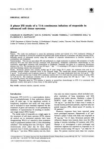
where D is the diffusion coefficient. Eq. (3.1) shows that the likelihood that particles travel further increases when either D or τ increases. While keeping D constant, this concept can be made clear using isocontours such that P (R; τ ) = c with c > 0. Figure 3.1 shows the same isocontour for diffusion times τ1 < τ2 < τ3 in four schematic representations of different tissue types. As can be seen by the growth of the isocontours, using longer τ increases the likelihood that particles travel further. The shape of the isocontour depends on the structure of the surrounding tissue. From left to right, in free water, where Eq. (3.1) is a good approximation, particles are unrestricted and travel furthest with isotropic, Gaussian probability. Next, at a course diffusion scale, gray matter tissue can often be seen as generally unorganized and hinders diffusion equally in all directions [Jones, 2010]. For this reason, these tissues also produce isotropic contours, but smaller than those in free water. In axon bundles, here illustrated as gray lines, axons are mostly aligned with the bundle axis. Particle movement is restricted perpendicular to this direction and is relatively free along it, causing anisotropic isocontours [Le Bihan and Breton, 1985, Taylor and Bushell, 1985, Merboldt et al., 1985]. Finally, in areas where two bundles cross there is a mix between the isocontours of each bundle. Note that we intentionally drew the isocontours for τ1 more isotropic than those of τ3 in the right two white matter tissues. For shorter τ , particles have not had much time to interact with surrounding tissue, resulting in a similar probability that a particle travels in any direction. The isocontours for very short τ will therefore always be isotropic. For longer τ , particles have had more time to interact with the tissue, either traveling far along a relatively unrestricted direction, or staying close to its origin along a restricted direction, resulting in more anisotropic profiles [Tanner, 1978]. When the tissue can be seen as axially symmetric (i.e. in a single bundle), this means that the perpendicular diffusivity D⊥ becomes τ -dependent and decreases as τ increases [Cohen and Assaf, 2002]. Different tissue types will ¨ induce different τ -dependence of the EAP [Ozarslan et al., 2006, 2012].


τ1 τ2

Free Water

τ3

Gray Matter

Coherent Bundle

Crossing Bundles

Figure 3.1: Schematic representations of different tissue types with their corresponding P (R; τ ) isocontours for different diffusion times τ1 < τ2 < τ3 . Longer τ increases the likelihood that particles travel further, indicated by the smaller blue isocontour for τ1 to the largest red isocontour for τ3 . The shape of the isocontour depends on the structure of the surrounding tissue. Diffusion is considered free in free water, hindered in gray matter and restricted in white matter bundles. Image inspired by Alexander [2006].

Figure 3.2: left: Diagram showing principal systems of association fibers in the cerebrum, connecting different cortical areas with a given hemisphere. right: the hemispheres of the brain, the fornix and corpus callosum bundles connecting the two. The white areas represent the white matter and the outer grey areas the Grey Matter. From 20th U.S. edition of Gray’s Anatomy of the Human Body (public domain).

3.2. DIFFUSION ANISOTROPY: THE PHENOMENON

3.2.2

39

Microstructure in the Brain

Images such as those in Figure 3.1 are useful to illustrate general properties of different brain tissues. However, it is important to realize that these are extreme simplifications. While this thesis concerns itself mainly with the estimation of tissue microstructure at the millimeter level (see Section 3.3), it is good to keep in mind that all our contributions are part of a larger ensemble of higher-order functions. To give an overview of the brain, Figure 3.2 shows schematic representations of the principal systems of association fibers and a horizontal cross-section of the brain, showing the two hemispheres. In broad terms, white matter (WM) is mainly composed of axonal nerve fibers, covered by a myelin sheath giving its distinctive color. It is found in the inner layer of the cortex, the optic nerves, the central and lower areas of the brian and surrounding the central shaft of grey matter in the spinal cord. Grey matter (GM) can be seen as mainly consisting of neurons and their unmyelinated fibers. Though strictly speaking, the terms gray and white matter are only valid in the context of gross anatomy. GM is only distinguished from WM, in that GM contains numerous cell bodies and relatively few myelinated axons. WM is composed chiefly of long-range myelinated axon tracts and contains relatively very few cell bodies. The brain also contains glial cells of various kinds who support the functioning of neurons. We illustrate the difference between gray and white matter microstructure in Figure 3.3. Focusing on the electron micrograph of the cross-section of the white matter bundles, it can be seen that while axons are often near-tubular, their diameter, amount of myelination and the space between them varies significantly. Axon Diameter and Myelination Axons are the structural and physiological conduit for signal transmission in the brain and therefore are one of the fundamental elements of brain function. The conduction velocity of nerves is directly related to axon diameter in both myelinated and unmyelinated axons [Hursh, 1939, Waxman, 1980, Hoffmeister et al., 1991]. Hursh [1939] showed the conduction velocity to be proportional to the square root of the diameter of unmyelinated axons and directly proportional to the inner membrane diameter of myelinated axons. In the peripheral nervous system, axon diameters range from 0.1 µm to about 20 µm, with unmyelinated axons being smaller than 2 µm and myelinated axons larger than 1 to 2 µm [Waxman and Kocsis, 1995]. In the central nervous system, myelinated axons diameters as small as 0.2 µm have been observed [Waxman, 1978], with axons below this size generally being unmyelinated. In particular, histology studies have determined that axon diameter distributions in the corpus callosum range between 0.2 and 2µm [Lamantia and Rakic, 1990, Aboitiz et al., 1992]. Variations in axon diameter are thought to be closely tied to function, with networks that demand fast response (such as motor networks) demonstrating


Electron Micrograph

Schematic Grey Matter

White Matter

Grey Matter

White Matter Cross-Section

5μm

2μm

Figure 3.3: The left image illustrates globally the different structure between gray and white matter; gray matter consisting mostly of cell bodies, white matter consisting mostly of fiber tracts, and both tissues containing many glial cells. On the right, we show two electron micrograph images of gray matter (adapted from [Kay et al., 2013]) and a cross-section of a white matter bundle (adapted from [Liewald et al., 2014]). The gray matter appears unorganized with many differently shaped cell bodies. The cross-section of the white matter bundles shows that while axons are often tubular, their diameter, amount of myelination and the space between them varies significantly.

larger axon diameters.

Axon Orientation Dispersion Histology studies show that the orientations of individual axons are often dispersed around the main bundle axis [Leergaard et al., 2010, Ronen et al., 2014]. While axon diameter and myelination are intrinsic tissue properties (as in they are properties of one axon), axon dispersion is more of a secondary property that arises by considering ensembles of axons. The presence of axon dispersion in coherent white matter (e.g. the corpus callosum) has been proven in recent years [Leergaard et al., 2010, Budde and Annese, 2013, Mollink et al., 2016], and is illustrated in results of other works as shown in in Figure 4.3. In general, the term axon orientation dispersion is used to describe any metric that quantifies the amount of misalignment of these axons within a finite measurement volume. In Microstructure Imaging, the estimation of axon dispersion or fanning is usually an interpretation of one or more concentration parameters of a spherical distribution of sticks or cylinders (See Chapter 4). However, in the next section, we will first go into more detail on how diffusion MRI can be used to measure a signal that is related to the tissue structure and the EAP.

3.3. DIFFUSION-WEIGHTED MAGNETIC RESONANCE IMAGING

From: Leergaard et al. PLOS ONE 2010

41

From: Mollink et al. ISMRM 2016

Figure 3.4: Histology, Polarized Light Imaging (PLI) and Diffusion MRI all confirm the presence of axon orientation dispersion in the corpus callosum of rats and humans. The left image is from Leergaard et al. [2010], showing a close-up of dispersed axon in the corpus collosum of a rat. The right image is from Mollink et al. [2016], where PLI and diffusion MRI both confirm the presence of significant orientation dispersion in the human corpus callosum.

3.3

Diffusion-Weighted Magnetic Resonance Imaging

In this section we explain the basic concepts needed to understand diffusion MRI. In particular, we discuss nuclear magnetic resonsance in Section 3.3.1, the basic underpinnings of diffusion MRI and the EAP in Section 3.3.2, the concept of diffusion restriction Section 3.3.3 and finally different acquisition schemes in Section 3.3.4.

3.3.1

Basics of Magnetic Resonance Imaging

Magnetic resonance imaging (MRI) is a medical imaging technique which is able to non-invasively obtain detailed information of internal structures in the body. It does this by exploiting the nuclear magnetic resonance (NMR) properties of 1 H nuclei, which are abundantly present in water and fatty tissues. An MRI scanner works by exposing a sample (in our case the brain) to a powerful magnetic field that is generated along the magnet bore. This magnetic field is called the B0 field, formally described as B0 = B0 v with B0 the magnetic field strength in Tesla (T) and v ∈ S2 the direction of the field. In the presence of the B0 field, the magnetic spins of 1 H nuclei will align with v and precess with Larmor frequency ω (see Figure 3.5a). The Larmor frequency depends on the strength of B0 and the gyromagnetic ratio of the proton γ such that ω = B0 γ

(3.2)


(a) Spin precession

(b) Rotating frame of reference

Figure 3.5: Schematic illustrations of basic MRI principles. (a) shows an aligned spin precessing with Larmor frequency ω. (b) shows the rotating frame of reference in which magnetization of spins is described. where γ = 42.58 MHz/T for 1 H. When all spins have aligned with the B0 field, a bulk magnetization M exists along v. To describe this magnetization, it is cumbersome to describe every spin separately. It is more convenient to describe the average magnetization of groups of spins experiencing the same magnetic field strength. These groups are called spin packets. In MRI, every voxel in the image represents such a spin packet. For every spin packet, M can be described in a rotating frame of reference (see Figure 3.5b). In this setting, M is composed of a longitudinal component Mz , which is aligned with B0 and a transversal component Mxy . When spins are in equilibrium, the magnetization only has an Mz component, whose magnitude depends on the number of protons in the spin packet and the strength of B0 . Using a receiver coil, the magnetization in the transversal plane can be measured. The scanner can then emit a radiofrequency (RF) pulse to tip M towards the transversal plane. The RF pulse is designed to have the Larmor frequency to tip the magnetization correctly and the duration of the pulse determines how far the magnetization is tipped. When the RF pulse is turned off, all the spins in a spin packet are in phase and the bulk magnetization will start to realign with B0 . This process is governed by two relaxation processes called T1 spin-lattice relaxation and T2 spin-spin relaxation. T1 spin-lattice relaxation describes the recovery of magnetization in Mz , while T2 spin-spin relaxation describes the decay of magnetization in Mxy . How fast these relaxation processes occur is determined by relaxation times T1 and T2 , where T2 is always shorter than T1 . After application of the RF pulse, the longitudinal and transversal relaxation of magnetization over time can be described by Mz (t) = Mz,eq − (Mz,eq − Mz (0))e−t/T1 ) and Mxy (t) = Mxy (0)e−t/T2

(3.3)

where Mz (t) and Mxy (t) are the longitudinal and transversal magnetization in Mz and Mxy at time t, Mz,eq is the longitudinal magnetization in equilibrium, Mz (0)


(a)

43

(b)

Figure 3.6: A filled k-space image (a) with its corresponding image after inverse Fourier transform (b). and Mxy (0) are the longitudinal and transversal magnetization immediately after the RF pulse and T1 and T2 are given in seconds. At a given time t the measured signal in the transversal plane can then be described by Z S(t) = ρ(y) · Mxy (y, t) · e−iωt dy (3.4) y∈R3

where S(t) is the measured signal, ρ(y) is the proton density at position y ∈ R3 , Mxy (y, t) is the transversal magnetization and e−iωt describes the oscillation of spins in the transversal plane with Larmor frequency ω. However, this “global” signal does not contain information on individual spin packets, i.e. it sees the whole sample as one voxel. To be able to receive a signal related to local structure in the sample, a so-called gradient field K given in T/m is used, where the gradient field consists of three orthogonal gradients such that K(y, t) = [Kx (y, t), Ky (y, t), Kz (y, t)]. These gradient fields influence the Larmor precession of spins position dependently such that ω(y, t) = γkB0 + K(y, t)k

(3.5)

where ω(y, t) is the Larmor frequency at position y and time t. Moreover, every gradient has a specific function. Here Kz enables slice encoding, Kx is known as the readout gradient and enables frequency encoding and Ky enables phase encoding. Together these gradients enable the encoding of a Fourier representation of an image known as k-space. When k-space has been filled with acquisition samples an inverse Fourier transform can be used to obtain the real image of the selected slice. Figure 3.6 shows a k-space with its accompanying reconstructed image. This process can be repeated for different slices to construct a 3D volume.


90°

180°

RF

δ diffusion gradient

time

δ G

G time

Δ echo

FID signal

time

TE/2

TE/2

Figure 3.7: Schematic illustration of the pulsed gradient spin echo sequence. The sequence is represented as the time evolution, i.e. occurrence and duration, of radiofrequency pulses (RF) in the first line, diffusion gradient pulses in the second line, and measured signal in the third line. The illustration reports the 90◦ and 180◦ RF pulses separated by half the echo-time TE, two diffusion gradient pulses of strength G and duration δ separated by a time ∆, and the free induction decay (FID) and echo of the measured signal.

3.3.2

Diffusion Weighted Imaging

The estimation of diffusion anisotropy can be thought of, in first approximation, as the assessment of the amount of preference that the diffusion process has for a specific spatial direction in terms of diffusivity. Therefore, this assessment requires sensing the diffusion signal along multiple spatial directions, regardless of the representation adopted to describe the signal itself. In MRI, this is typically done by acquiring a collection of images of the target object, e.g. the brain. Each image is acquired when the experimental conditions within the magnet’s bore determine a specific diffusion-weighting along the selected spatial direction: this is a DiffusionWeighted Image (DWI). The diffusion-weighting is globally encoded by the b-value [Le Bihan and Breton, 1985], measured in s/mm2 , a quantity that is the reciprocal of the diffusivity, D (mm2 /s). The intensity of the diffusion-weighting, i.e. the b-value, is determined by the acquisition setup. The most common type of acquisition is the Pulsed Gradient Spin-Echo sequence (PGSE) [Stejskal and Tanner, 1965], where a DWI is obtained by applying two diffusion gradients with intensity G = kGk (T/m) and pulse length δ (s) to the tissue, separated by the separation time ∆ (s). We illustrate this sequence in Figure 3.7. The resulting signal is ‘weighted’, along the applied gradient direction,


45

with b-value [Stejskal and Tanner, 1965] 2

2 2

b=γ G δ

δ ∆− 3

(3.6)

where γ (MHz/T) is again the nuclear gyromagnetic ratio of the water proton 1 H. The measurement of the diffusion signal is directly related to the concept of attenuation. Indeed, in the presence of diffusion, the signal intensities S(b) of the voxels of a DWI are lower than the corresponding intensities when the image is acquired without diffusion-weighting S0 = S(0). Along the selected gradient direction, the quantity E(b) = S(b)/S0 expresses, for each voxel, the attenuation of the diffusion-weighted signal. In the absence of restrictions to the diffusion process, the attenuation is [Stejskal and Tanner, 1965] E(b) =

S(b) = e−bD , S0

(3.7)

which expresses an exponential attenuation profile, as is illustrated in Figure 3.8a. In the case of the PGSE sequence, this attenuation phenomenon can be interpreted as the result of a differential mechanism. The sequence, shown in Figure 3.7, starts with a 90◦ radio-frequency pulse after which it is possible to measure a signal, namely Free Induction Decay (FID), that is related to the macroscopic spins’ net magnetization. After a time TE/2, with TE the echo-time, a second 180◦ radiofrequency pulse has the effect of generating an echo of the signal whose peak is at time TE, corresponding to the end of the sequence [Hahn, 1950]. The first diffusion gradient pulse is applied between the two radio-frequency pulses. Here, we assume the narrow gradient pulse condition δ ∆, which implies that spins are static during the application of the gradient pulses [Tanner and Stejskal, 1968]. Under this assumption, after the first gradient pulse, a spin located at position r1 is subject to a phase accumulation φ1 = γδG · r1 . After a time ∆ from the start of the first gradient pulse, and after the 180◦ radio-frequency pulse, a second gradient pulse of equal magnitude and duration to the first is applied. If the spin has moved to a position r2 the phase accumulation during the second pulse is φ2 = γδG · r2 . However, the 180◦ radio-frequency pulse has the effect of changing the sign of the second gradient pulse. Therefore, at the end of the sequence, i.e. at the echo-time TE, the spin has acquired a net phase shift φ = φ2 − φ1 = γδG · (r2 − r1 ) = γδG · r

(3.8)

which is null in the case the spin remained static, i.e. r = r2 − r1 = 0. The signal attenuation takes into account an ensemble of spins and can be related to the ensemble average propagator (EAP), P (r, τ ), via a Fourier relationship under the q-space formalism [Tanner and Stejskal, 1968, Callaghan, 1991] Z E(q, τ ) = P (r, τ )ej2πq · r dr (3.9) R3

46CHAPTER 3. MICROSTRUCTURE, DIFFUSION PROPAGATOR AND ANISOTROPY where q is the wave vector and τ is diffusion time, which for the PGSE sequence are expressed as γδG q= and τ = ∆ − δ/3. (3.10) 2π These quantities influence differently the diffusion-weighting, i.e. the b-value. Indeed, the wave frequency q = kqk is expressed in mm−1 and is the reciprocal of the spins displacement r = krk expressed in mm. As such, q is a spatial frequency, and by increasing its value it is possible to achieve a higher spatial resolution of P (r, τ ) in the displacement space described by r. In addition, the diffusion time τ expresses the time interval during which spins are allowed to diffuse before measurement.

3.3.3

Diffusion Restriction

A longer diffusion time allows the spins to move a longer distance causing, in the absence of restrictions to the diffusion process, a larger net phase shift, i.e. a stronger attenuation of the signal. Therefore, expressing the diffusion-weighting in terms of q and τ can provide useful insights on the signal nature. In the absence of restrictions to the diffusion process, eq. (3.9) has a closed form. This is obtained by substituting q and τ of eq. (3.10) into the formulation of the b-value expressed in eq. (3.6), such that b = 4π 2 q 2 τ and eq. (3.7) becomes E(q, τ ) = e−4π

2 q2 τ D

(3.11)

which expresses a Gaussian attenuation profile as function of q. However, Eqs. (3.7) and (3.11) are valid when the diffusion process can be considered unrestricted, e.g. when the movement of spins is not obstructed by the presence of a barrier. In the case of restricted diffusion, for instance when the signal is measured along a direction perpendicular to a barrier, these equations are no longer valid. Unrestricted and restricted scenarios are depicted by the schematic representation in the left side of Figure 3.8, where the diffusion process occurs between two parallel barriers, i.e. the restriction, and where two arrows represent the measurement directions parallel and perpendicular to the restriction. The figure also illustrates the signal attenuation in the case of parallel, unrestricted diffusion (a,b), and in the case of perpendicular, restricted diffusion (c,d ). The unrestricted attenuations are obtained with eqs. (3.7) and (3.11), whereas the restricted ones are simulated as the diffusion signal attenuation generated within an ensemble of cylinders along the direction perpendicular to the cylinders’ axes [Callaghan, 1995]. Moreover, the curves in a and c are reported as function of the b-value with diffusion time τ2 , whereas the curves in b and d are functions of the q-value and are reported for increasing diffusion times τ1 < τ2 < τ3 . In the graphs, points of each curve corresponding to b = 1000 s/mm2 are highlighted with a dot. Along the unrestricted direction (a,b) the attenuation values, indicated by dots, are lower than the corresponding ones along the restricted direction (c,d ). Indeed,

3.3. DIFFUSION-WEIGHTED MAGNETIC RESONANCE IMAGING a

b

c

d

47

Parallel unrestricted

Perpendicular restricted

Figure 3.8: The effect of b-value, q-value and diffusion time on the signal attenuation when diffusion is unrestricted or restricted by the presence of a barrier. The graphs report the signal attenuations along a direction parallel to the restriction (a,b) – represented by two black barriers in the schematic image – and along the perpendicular direction (c,d ), where the diffusion process is restricted. The attenuations are reported as function of the b-value (a,c) with diffusion time τ2 , and q-value (b,d ) for increasing diffusion times τ1 < τ2 < τ3 . Dots indicate the attenuation measured at b = 1000 s/mm2 .

when diffusion is restricted by the presence of the barrier, the spins are subject to a smaller net displacement and the signal attenuates less. The choice of q and τ to obtain a certain diffusion-weighting, i.e. a specific b-value, assumes different relevance in terms of signal attenuation depending on whether diffusion is restricted or not. In the absence of restrictions (a,b), an increase of q-value or diffusion time always attenuates the signal, and points with different q and τ , but with same b-value, render the same amount of attenuation (b). However, when diffusion is restricted (c,d ), an increase of the diffusion time τ implies letting the spins diffuse a longer distance with the consequence of experiencing more restriction. In this case, the Gaussian attenuation expressed by eq. (3.11) is not longer valid. Indeed, different combinations of q and τ render different non-Gaussian profiles of signal attenuation, and points with same b-value – the dots of Figure 3.8d – correspond to different attenuations.

3.3.4

Acquisition Schemes

The estimation of diffusion anisotropy, based on the diffusion signal attenuation along different gradient directions, depends on the chosen experimental parame-

48CHAPTER 3. MICROSTRUCTURE, DIFFUSION PROPAGATOR AND ANISOTROPY e

n sio

m Ti

Gradient Strength

ffu

Multi-Shell HARDI DTI

qτ-Acquisition

Di

G r a di e n

t

ec DIr

ti o

ns

Figure 3.9: Schematic for different types of acquisition schemes. DTI schemes are typically acquired at a low gradient strength, typically b < 1000 s/mm2 , for a minimum of 6 gradient directions. HARDI typically uses higher gradient strengths, typically b > 2000 s/mm2 with over 40 gradient directions. Multi-shell uses DTI and HARDI shells for a given diffusion time, and finally qτ -acquisitions are multi-shell acquisitions for a range of diffusion times.

ters, especially q and τ . Indeed, different sets of parameters lead to different signal attenuations – depending on the underlying diffusion process – and consequently to different measurements of anisotropy. Ideally, a complete characterization of anisotropy would require the measurement of the diffusion signal attenuation for many gradient directions, q-values, and diffusion times τ . However the optimal sampling is still under debate. In practice, with reference to diffusion anisotropy, the choice of how to sample the diffusion signal depends on the application and on the chosen signal representation. For instance, in DTI it is common practice to measure only one shell of gradient directions using a single b-value, as illustrated in Figure 3.9. High Angular Resolution Diffusion Imaging (HARDI) schemes, still measuring only one shell but at a higher b-value and more directions, are used to gain a higher angular resolution of the diffusion signal with the purpose of resolving crossing tissue configurations [Tuch et al., 2002]. Other signal representations require signal acquisition at different diffusion-weightings. A common choice, namely multi-shell, consists in acquiring different q-shells while fixing the diffusion time. Each shell represents a collection of samples in the three-dimensional space with the same q-value. These samples can be imagined as lying on a sphere, as shown in Figure 3.9, where an optimal spatial coverage is important to measure the diffusion signal as efficiently as possible. This concept can be expanded over multiple shells

3.4. THE INTER-MODEL VARIABILITY OF DIFFUSION ANISOTROPY 49

FADTI

PADTI

GFAQ-ball

PAMAPMRI

GFAMAPMRI

μFASMT

1-ODINODDI

Figure 3.10: Visualization of various normalized measures describing diffusion anisotropy, where the corresponding model is given in the subscript. In the top row, we show Fractional Anisotropy (FA) and Propagator Anisotropy (PA) of Diffusion Tensor Imaging (DTI), PA by Mean Apparent Propagator (MAP)-MRI and micro-FA by Spherical Mean Technique (SMT). In the bottom row, we show Generalized Fractional Anisotropy (GFA) by Q-ball Imaging and by MAP-MRI and finally one minus the Orientation Dispersion Index (ODI) by Neurite Orientation Dispersion and Density Imaging (NODDI). The complement of ODI is shown for overall coherence, since high ODI normally indicates low anisotropy.

such that all of the acquired samples lie on different non-collinear directions [Caruyer et al., 2013]. The multi-shell concept can be extended to τ -shells, called a qτ acquisition [Fick et al., 2016c], since nowadays there exist signal representations that exploit different value for both q and τ . In this case, a complete q-shell scheme – with samples distributed along different gradient directions and with different diffusion-weightings – is acquired for each desired diffusion time.

3.4

The Inter-Model Variability of Diffusion Anisotropy

As the subject of this thesis is microstructure imaging, it is appropriate that we start with addressing the metric that is most commonly used as a marker for changes in tissue microstructure: diffusion anisotropy. Simply meaning “deviation from diffusion isotropy”, different interpretations of diffusion anisotropy have been proposed using different acquisition requirements and mathematical underpin¨ nings [Basser, 1995, Tuch, 2004, Ozarslan et al., 2013b, Kaden et al., 2015]. Out of these, the clinical applications of Fractional Anisotropy (FA) [Basser, 1995] of the Diffusion Tensor Imaging (DTI) model [Basser et al., 1994] has been most widely

50CHAPTER 3. MICROSTRUCTURE, DIFFUSION PROPAGATOR AND ANISOTROPY explored. Changes in FA have been related to brain diseases such as ischemia, multiple sclerosis, trauma, brain tumors and many more [see e.g. reviews by Assaf and Pasternak, 2008, Soares et al., 2013]. For this reason, FA is seen as a “potential biomarker” for these disease patterns, where biomarker is a portmanteau of “biological marker” [Strimbu and Tavel, 2010]. However, the fact that FA is sensitive to all these processes also means that it is specific to none of them. Diffusion anisotropy measures, as a rule of thumb, always have the following three properties: • They are rotationally invariant, i.e., insensitive to rotations. • They are normalized, with zero being the lowest measure for diffusion anisotropy and one being the highest. • They somehow describe “deviation from diffusion isotropy”. The last point is intentionally left open to interpretation, which is exactly the point we are making in this section. To illustrate this, we discuss five different anisotropy measures; Fraction Anisotropy (FA) [Basser, 1995], Generalized Frac¨ tion Anisotropy (GFA) [Tuch, 2004]; Propagator Anisotropy (PA) [Ozarslan et al., 2013b]; Orientation Dispersion Index (ODI) [Zhang et al., 2012]; and microscopic Fractional Anisotropy (µFA) [Kaden et al., 2015]. While assessing the validity of the interpretation of diffusion anisotropy for different disease patterns is beyond the scope of this work, we will address the ambiguity of its estimation. This section is therefore meant as a simultaneous overview of, and discussion on, current methods that estimate diffusion anisotropy measures or anisotropy-related tissue properties. We start this section by first detailing the data of the Human Connectome Project [Setsompop et al., 2013] that we use to illustrate different diffusion anisotropy measures in Section 3.4.1. We then describe the inter-model variability of the mathematical definition and estimation of diffusion anisotropy in Sections 3.4.2 through 3.4.6. The anisotropy measures of all presented techniques are qualitatively and quantitative compared in Figures 3.10, 3.11 and 3.12.

3.4.1

Data Set Description and Adopted Notation

We use the MGH Adult Diffusion Data of the Human Connectome Project to illustrate different measures of diffusion anisotorpy [Greve and Fischl, 2009, Andersson et al., 2012, Keil et al., 2013, Setsompop et al., 2013]. This data set was acquired at particularly high b-values {0, 1000, 3000, 5000, 10000} s/mm2 with {40, 64, 64, 128, 256} directions, respectively. The diffusion time and pulse separation time in this data are δ/∆ = 12.9/21.8 ms with 1.5 × 1.5 × 1.5 mm resolution and T E/T R = 57/8800 ms.


Region Of Interest ROI Anisotropy

1.0

Crossing

CSF

Single Bundle

0.8 0.6 0.4 0.2

FA _D PA TI GF _D A T GF _M I A_ AP Q 1- PA ba OD _ ll I_N MA P μF ODD A_ SM I T



0.0

Figure 3.11: Box-plots of estimated anisotropy measures in different regions of interest, indicated as the different colors in the coronal brain slice in the right corner. We illustrate anisotropy in free water (CSF), a single bundle (Corpus Callosum) and a crossing area (Centrum Semiovale). It can be seen that the same metric for different techniques, or different metrics for the same technique can result in different estimates of anisotropy. To briefly recap and clarify what notation we use, we denote that the signalbased models in this section directly estimate the EAP P (R; τ ) from the measured signal attenuation E(q, τ ), using the Fourier relationship in Eq. (3.9). Notice that P (R; τ ) is a conditional probability density for diffusion time τ , as the Fourier transform is only over the q, R space. We will interchangeably use real displacement vector R = ru with its distance and direction r ∈ R+ , u ∈ S2 and q-space vector q = qn with its q-space distance and gradient orientation q ∈ R+ , n ∈ S2 . The following anisotropy measures are then defined as some difference or ratio between the isotropic and anisotropic parts of P (R; τ ).

3.4.2

Fractional Anisotropy

Starting with the oldest measures for diffusion anisotropy, FA [Basser, 1995] is specific for the DTI model [Basser et al., 1994]. DTI solves the Fourier transform by generalizing the Stejskal-Tanner equation for unbounded media [Tanner and Stejskal, 1968] to three dimensions: E(b, n) = exp(−bnT Dn)

or E(q, τ ) = exp(−4π 2 q 2 τ nT Dn)

(3.12)

with D a 3 × 3 symmetric positive-definite diffusion tensor. Notice that Eq. (3.12) is Gaussian over q and exponential over τ , which will be important in studying time-dependence in Section 3.5. FA describes fraction of the “magnitude” of D

52CHAPTER 3. MICROSTRUCTURE, DIFFUSION PROPAGATOR AND ANISOTROPY that we can ascribe to anisotropic diffusion in terms of its eigenvalues {λ1 , λ2 , λ3 } as r p 1 (λ1 − λ2 )2 + (λ2 − λ3 )2 + (λ3 − λ1 )2 std(λ) p . (3.13) FA = = rms(λ) 2 λ21 + λ22 + λ23 We illustrate FA in a cross-section of the HCP data in Figure 3.10. The interpretation of FA has known limitations as DTI cannot represent crossing tissue configurations, but finds some average, Gaussian approximation that best fits the overall signal [Basser et al., 1994]. We illustrate this by estimating DTI’s Orientation Distribution Function ODF(u; τ ), representing the probability density that a diffusing particle will travel along direction u by marginalizing r as Z ∞ P (ru; τ )r2 dr (3.14) ODF(u; τ ) = 0

where r2 is the Jacobian of the radial integration to ensure that the integral of the ODF is unity [Trist´ an-Vega et al., 2009, Aganj et al., 2010]. Notice that Eq. (3.14) is general, and can be used for any method that estimates P (ru; τ ). For instance, Eq. (3.14) can be given analytically for DTI as ODFDTI (u) =

1 1 2

3

4π|D| (uT D−1 u) 2

.

(3.15)

We show DTI’s ODFs in a crossing area in Figure 3.12, where it can be seen that round profiles with low FA are found where other methods detect crossings.

3.4.3

Generalized Fractional Anisotropy

As a more general form of diffusion anisotorpy is Generalized Fractional Anisotropy (GFA) [Tuch, 2004]. GFA was proposed for High Angular Resolution Diffusion Imaging (HARDI) techniques [Tuch et al., 2002] that estimate ODFs capable of representing crossing tissue configurations [Tuch et al., 2003]. It is noteworthy that the only difference between DTI and HARDI is that in HARDI more gradients g are measured at a higher b-values, see Figure 3.9. This means that still no radial information is known of P (ru; τ ), and Gaussian decay over r is assumed to estimate the ODF in Eq. (3.14). For any ODF, the GFA is given as s P n ni=1 (ODF(ui ) − ODF)2 std(ODF) P = GFA = (3.16) rms(ODF) (n − 1) ni=1 ODF(ui )2 where ODF (u) is the value of the ODF in direction u, n is the number of evaluated ODF directions and ODF is the mean ODF intensity. We show Q-ball Imaging ODFs [Tuch, 2004, Descoteaux et al., 2007a, Aganj et al., 2010] in the top-right of Figure 3.12, where now crossing structures can be seen. Though, it must be said that FRT has been applied to a variety of HARDI methodologies, a selection


ODFs / FODs in Crossing Area for Different Methods DTI ODFs with FA Background

Q-ball ODFs with GFA Background

MAPMRI ODFs with PA Background

SMT FODs with μFA Background

Watson ODFs with 1-ODI Background

Figure 3.12: Orientation Distribution Functions (ODFs) for DTI, Q-ball, MAPMRI, the Watson distributions of NODDI and Fiber Orientation Distributions (FODs) of SMT in an area where it is known there are crossing bundles. Each method has its corresponding anisotropy measure as background texture. It can be seen that DTI finds an average orientation, where Q-Ball, MAPMRI and SMT find crossing structures. The FODs, being the result of a deconvolution, show sharper peaks, and more consistent crossings than the ODF techniques. It is important to realize that while NODDI separates the signal contributions of intra- and extra-axonal diffusion, its dispersion index jointly describes the spread of both of these compartments, and produces very similar ODFs as DTI.

54CHAPTER 3. MICROSTRUCTURE, DIFFUSION PROPAGATOR AND ANISOTROPY of which is summarized in Tristan-Vega et al. [2010]. Moreover, notice that GFA intensities in the crossing and single bundles areas are more similar than seen with DTI’s FA in the top-left, but the overall intensities of GFA and FA are different. We illustrate this by comparing estimated anisotropy intensities in different ROIs, for different measures and techniques in Figure 3.11. It can be seen that the same metric for different techniques, or different metrics for the same technique can result in different estimates of anisotropy.

3.4.4

Propagator Anisotropy

PA was proposed for the multi-shell, Mean Apparent Propagator (MAP)-MRI tech¨ nique [Ozarslan et al., 2013b]. MAP-MRI can be seen as a generalization of DTI, and allows for the estimation of three-dimensional P (ru; τ ), where now both restricted (non-Gaussian) diffusion over r and crossing axons can be represented. MAP-MRI is not unique in this respect, as a plethora of multi-shell techniques have been proposed for this purpose [See e.g. Assemlal et al., 2009, Descoteaux et al., 2011, Hosseinbor et al., 2013, Rathi et al., 2014], but MAP-MRI’s formulation allows for easy estimation of a large variety of q-space properties using efficient regularization [Fick et al., 2016d]. PA is defined as the a measure of dissimilarity between the reconstructed P (R; τ ) and its closest isotropic approximation Piso (R; τ ). First, the inner product between two EAPs is defined as Z hP (R; τ )Piso (R; τ )i = P (R; τ )Piso (R; τ )dR (3.17) R3

The similarity between two propagators is measured as an angular measure of covariance in analogy with the vector product [Avram et al., 2015]: s cos θPA =

hP (R; τ )Piso (R; τ )i hP (R; τ )P (R; τ )ihPiso (R; τ )Piso (R; τ )i

PA is then defined using the angular dissimilarity measure sin θPA = and scaling function σ(t, ) as PA = σ(sin θPA , 0.4)

with σ(t, ) =

t3 . 1 − 3t + 3t2

(3.18) q 2 1 − cos θPA

(3.19)

¨ where we note that scaling parameter = 0.4 was chosen by Ozarslan et al. [2013b] to yield “the desired level of contrast in real images”. PA can be estimated for any method that reconstructs P (R; τ ). For instance, for DTI it is given as 2 cos θPA-DTI =

8u30 ux uy uz (u2x + u20 )(u2y + u20 )(u2z + u20 )

(3.20)

3.4. THE INTER-MODEL VARIABILITY OF DIFFUSION ANISOTROPY 55 where the displacement is given as a function of DTI’s eigenvalues as{ux , uy , uz } = p ¨ 2τ {λ1 , λ2 , λ3 } [Basser, 2002], and u0 is DTI’s nearest isotropic propagator [Ozarslan et al., 2013b]. We show PAMAPMRI and PADTI in Figures 3.10 and 3.11, where this measure indeed seems to show good contrast between isotropic, crossing and single bundle tissues.

3.4.5

Orientation Dispersion Index

As the only multi-compartment model that we consider in this chapter, the neurite orientation dispersion and density imaging (NODDI) model [Zhang et al., 2012] parameterizes diffusion anisotropy as the dispersion of the diffusion signal of individual axon segments around a central bundle axis. In NODDI, axons as are represented as sticks – cylinders with zero radius and parallel diffusivity λk – and are dispersed according to a Watson distribution W (κ, µ), where κ is the concentration parameter that is inversely related to axon dispersion, and µ ∈ S2 is the bundle direction. NODDI also separates the signal contribution of the Cerebrospinal Fluid (CSF) as an isotropic Gaussian with diffusivity Diso (i.e. a Ball) and the hindered hindered extra-axonal compartment – the diffusion directly around the axons – as an axially symmetric Tensor (i.e. a Zeppelin) with parallel and perpendicular diffusivity λext k . The overall signal representation is then and λext ⊥ NODDI EWatson

  Zeppelin Ball Watson Stick }| { z z }| { z }| { z }| {   ext = fCSF Eiso (DCSF ) + W (κ, µ) ∗S2  fh Eh (λext ⊥ , λk ) + fr Er (λk )  {z } | | {z } | {z } CSF

Hindered Extra-Axonal

(3.21)

Intra-Axonal

where the volume fractions of the CSF, hindered and intra-axonal compartment sum up to unity as fCSF + fh + fr = 1, and ∗S2 represents the spherical convolution that distributes the per-axon diffusion signal (both the stick and the hindered compartment) according to the Watson distribution. In practice, NODDI fixes all diffusivities of the different model components and focusses on the estimation of κ, µ and the volume fractions. We leave a more detailed description and discussion on NODDI for Chapter 4. NODDI reparameterizes the concentration parameter κ into the normalized Orientation Dispersion Index (ODI) ODI =

2 arctan(1/κ) π

(3.22)

where ODI = 0 now means no dispersion, i.e. parallel axons and therefore high diffusion anisotropy, and ODI = 1 represents completely dispersed (isotropic) diffusion. We fitted the NODDI model using the NODDI toolbox1 and illustrate the complement of ODI in Figures 3.10 and 3.11. It can be seen that the contrast of previously discussed signal-based anisotropy measures and ODI is quite similar. Figure 3.12 also shows the ODFs of the estimated Watson distributed, which resemble the DTI ODFs in many cases. 1

http://www.nitrc.org/projects/noddi_toolbox


3.4.6

Microscopic Fractional Anisotropy

Similarly as NODDI, the Spherical Mean Technique (SMT) [Kaden et al., 2015] also represents the diffusion signal as a distribution of individual axon segments with a spherical Fiber Orientation Distribution FOD(n). However, unlike NODDI, SMT does not do any separately model the hindered and CSF compartments, nor does it assume any parameterization of the FOD, and only assumes that the FOD is a R probability density such that S2 FOD(n)dn = 1 and the individual axon segment is represented by an axially symmetric tensor with perpendicular and parallel diffusivity λ⊥ and λk . It then follows that, for a given b-value, the spherical integral of the overall diffusion signal Eb (n) and that of the individual axon segment Kb (n) must be equal such that Z Z Z Kb (n)dn = K (b, λ⊥ , λk ). (FOD ∗S2 Kb )(n)dn = Eb (n)dn = E (b) = S2

S2

S2

(3.23) It is possible to solve this equation for λ⊥ and λk using constrained least squares such that 0 < λ⊥ < λk < λfree with λfree the free water diffusivity. Once λk , λ⊥ are known, the per-axon fractional anisotropy (µFA) is calculated as in Eq. (3.13), with λ1 = λk and λ2 = λ3 = λ⊥ . As we show in Figures 3.10 and 3.11, the estimation of µFA in the SMT framework is now independent of axon dispersion or crossing tissue configurations, that are very noticeable in for instance FA and ODI. Also, the per-voxel FOD can now be obtained using standard techniques such as Constrained Spherical Deconvolution [Tournier et al., 2007], allowing for the recovery of very sharp orientation profiles as shown in Figure 3.12.

3.5

Sensitivity of Anisotropy to Diffusion Time

Recent work has put focus on the diffusion time dependence of the diffusion coefficient [Fieremans et al., 2016]. When this effect has an orientational dependence, it also directly affects the estimation of diffusion anisotropy. To illustrate this, we use Camino [Cook et al., 2006] to simulate the diffusion signal in two substrates consisting of parallel axons – modelled as cylinders – with gamma distributed radii. We show cross-sections of these substrates in Figure 3.13. We simulate a multi-shell acquisition with two shells using b-values {1000, 3000} s/mm2 with 30 and 60 gradient directions, respectively, and one b0 image without diffusion weighting. We set pulse length δ = 1ms and vary pulse separation ∆ from 1ms to 40ms, while scaling the gradient strength to keep the b-values constant. While here we set δ constant to simplify the example, varying δ also influences the diffusion signal and its impact should not be ignored in practice [˚ Aslund and Topgaard, 2009]. We show the progress of FA, GFA and PA on the right of Figure 3.13 for both distributions. It can be seen that all metrics describe the signal becoming more

3.6. DISCUSSION

57

Camino Cylinder Distributions

1.00 0.95

Anis otropy

0.90 0.85 0.80

FA dis t 1 FA dis t 2 GFA dis t 1 GFA dis t 2 PA dis t 1 PA dis t 2

0.75 0.70 0.65 0.60

Distribution 1

Distribution 2

0.55

0

5

10

15

20

25

30

35

40

Diffus ion Tim e [m s ]

Figure 3.13: left: Cross-sections of Camino cylinder substrates with gammadistributed radii. Distribution 1 has smaller radii and less extra-cellular space than distribution 2. right: Diffusion time dependence of anisotropy measures from the two left distributions. The estimated anisotropy increases as longer diffusion times are used, until a plateau is reached.

anisotropic as diffusion time increases, even though different metrics report different levels of anisotropy. In all cases, distribution 1, having more densely packed, smaller axons, produces a more anisotropic signal.

3.6

Discussion

In the first parts of this chapter, we have first covered the basic concepts of brain microstructure and diffusion MRI. Critically, we illustrated diffusion is restricted by tissue boundaries, leading to time-dependent non-Gaussian diffusion (Figure 3.8). In tissues that restrict diffusion non-uniformly this leads to anisotropic diffusion profiles. The diffusion signal can furthermore be sampled using various acquistion schemes, ranging from single-shell DTI-schemes to multi-shell multi-diffusion time qτ -schemes (Figure 3.9). In second part of this chapter, we have discussed a range of diffusion anisotropy related measures, coming from either signal-based dMRI models that estimate the EAP from the signal as a whole, or models that use a multi-compartment approach to estimate axon dispersion. While these anisotropy measures have slightly different qualitative contrasts (Figure 3.10) and varying values in different tissue configurations (Figure 3.11), an important takeaway is that none of these metrics are better than any of the others from a methodological point of view. They all quantify diffusion anisotropy in some way. Arguably, an ideal measure for microstructure classification should be robust to as many acquisition parameters as possible, while still showing sensitivity and specificity to pathological changes [Vollmar et al., 2010]. As we illustrate in this chapter, these criteria are hard to meet for diffusion anisotropy for several reasons:

58CHAPTER 3. MICROSTRUCTURE, DIFFUSION PROPAGATOR AND ANISOTROPY 1. The definition of diffusion anisotropy changes for different dMRI models, as illustrated in Section 3.4. 2. The reproducibility of anisotropy measures is influenced by a variety of acquisition parameters, including, but not limited to, the number of gradient directions, signal-to-noise ratio, b-value, and voxel size [Barrio-Arranz et al., 2015], (Figure 3.13). 3. Different tissue configurations can produce the same level of estimated diffusion anisotropy (Figure 3.11). Nevertheless, diffusion anisotropy, and in particular fractional anisotropy (FA), has been related to a variety of pathologies, see e.g. the review by Assaf and Pasternak [2008]. However, only a few studies have shown the potential of using GFA [Cohen-Adad et al., 2011] or PA [Fick et al., 2016b], while large-scale comparisons like those for FA are missing. This can perhaps be attributed to the higher acquisition requirements that are required for HARDI and multi-shell techniques, making them less suitable for current clinical applications. Moreover, the typical criterium for being a biomarker is that the measure of interest should provide a statistically significant difference between healthy and diseased populations. However, care should be taken in prematurely calling a nonspecific marker such as diffusion anisotropy a biomarker. As an illustration, in the particular case of Parkinson’s disease, after many studies had claimed that FA could be used as a diagnostic biomarker, a systematic review of these studies actually showed that on its own, it cannot [Hirata et al., 2016]. It is likely that the non-specificity of diffusion anisotropy will continue to confound its interpretation as a biomarker for pathology. In an effort to improve specificity, NODDI’s multi-compartment approach using ODI has been shown to be more discriminative than DTI in normal human brain development and ageing [Chang et al., 2015], neurological disorders [Winston et al., 2014], brain connectivity [Lemkaddem et al., 2014] and Alzheimer’s disease [Nir et al., 2016, Colgan et al., 2016]. We will continue towards more advanced models of tissue microstructure that go beyond diffusion anisotropy in the next Chapter 4.

3.7

Conclusion

In the first two parts of this chapter, we provided a brief overview of the relationship between the ensemble average propagator (EAP) and the tissue microstructure. As the subject of this thesis is microstructure imaging, everything in the following chapters is based around this idea that the diffusion signal and the microstructure are linked. In the second part of this chapter, we provided the basic concepts in diffusion MRI to recover a diffusion weighted signal, ranging subjects between

3.7. CONCLUSION

59

basis NMR theory until acquisition scheme design. In particular, we focused on the Pulsed Gradient Spin Echo (PGSE) sequence, which is the main sequence we use in this thesis. In the last part of this Chapter, we have reviewed the inter-model variability of diffusion anisotropy estimation, as well as illustrated its sensitivity to especially short diffusion times. It is clear that there are many ways of defining diffusion anisotropy, depending on the chosen signal representation and acquisition scheme. It can be concluded that diffusion anisotropy is certainly a metric that, in combination with other indicators, can be used as a sign of neuropathology. However, on its own, it lacks specificity, which disqualifies it as being a true marker of tissue microstructure.


Chapter 4

PGSE-Based Microstructure Imaging: Can One Sense the Shape of the Brain Tissue?

Contents 4.1

Introduction

. . . . . . . . . . . . . . . . . . . . . . . . . .

62

4.2

Biophysical models of Tissue Microstructure . . . . . . .

63

4.3

4.4

4.5

4.6

4.2.1

Models of Intra-Axonal Diffusion . . . . . . . . . . . . . .

65

4.2.2

Models of Extra-Axonal Diffusion and Tortuosity . . . . .

68

4.2.3

Models of Axon Distribution . . . . . . . . . . . . . . . .

70

A Review on Microstructure Models . . . . . . . . . . . .

73

4.3.1

On Axon Dispersion Estimation . . . . . . . . . . . . . .

76

4.3.2

On Axon Diameter Estimation . . . . . . . . . . . . . . .

82

4.3.3

On “Apparent” Microstructure Measures . . . . . . . . .

85

Histology Validation of Microstructure Estimation . . .

88

4.4.1

Spinal Cord Data With Ground Truth Histology . . . . .

89

4.4.2

Validation of Intra-Axonal Volume Fraction . . . . . . . .

89

4.4.3

Validation of Axon Diameter . . . . . . . . . . . . . . . .

91

Discussion

. . . . . . . . . . . . . . . . . . . . . . . . . . .

94

4.5.1

Observed Trends and Challenges in Microstructure Imaging 94

4.5.2

On Histology Validation of Microstructure Estimation . .

96

4.5.3

Towards a Minimal Model of White Matter Diffusion . . .

98

Conclusion

. . . . . . . . . . . . . . . . . . . . . . . . . . . 102

Based on: Rutger H.J. Fick and Rachid Deriche “PGSE-Based Microstructure Imaging: Can One Sense the Shape of the Brain Tissue?” (In Preparation) 61

62

CHAPTER 4. CAN ONE SENSE THE SHAPE OF THE BRAIN TISSUE?

Overview In this Chapter we provide an extensive review, analysis and discussion on state-ofthe-art microstructure models. Every “microstructure” model uses a combination of “biophysical” models that each represent a particular part of the underlying tissue structure (e.g. intra- or extra-axonal). We deconstruct and classify microstructure models by their components and the microstructural interpretation they lend to their model parameters. In particular, we make a specific effort to expose the assumptions and limitations that each model has. We follow this with a validation of intra-axonal volume fraction and axon diameter estimation between different modeling approaches using spinal cord data with registered diffusion MRI and ground truth histology. We end this chapter by addressing current concerns about the degeneracy of the solutions of multi-compartment models when the diffusivities are not fixed, and propose a methodology that avoids this degeneracy.

4.1

Introduction

Can one sense the microstructure of the brain tissue using diffusion MRI? This is diffusion MRI’s seminal question that continues to drive the Microstructure Imaging community forward. It can be seen as a variant of the previously posed question Can One Hear The Shape of a Drum? by Bers and Kac [1966]. In his work, Kac explores the question of whether the shape of a drum can be inferred by the sound it makes, i.e., the frequencies it produces. Similarly, in diffusion MRI, we “hear” the frequencies of the ensemble average propagator (EAP) of water particles, represented as the measured diffusion signal, whereas the drum is represented by the surrounding tissue boundaries. Kac’s question was finally answered negatively by Gordon et al. [1992], who showed that two differently shaped drumheads could produce the same sound – as long as they produce the same frequency Eigenvalues. In other words, one cannot hear the shape of the drum completely, but still some information can be inferred. The analogy between Kac’s question and ours does not end here, as Jelescu et al. [2016] recently illustrated that ranges of estimated tissue configurations can produce the same diffusion signal, i.e., make the same sound. To understand the implications of Jelescu et al.’s work, this chapter is dedicated to understanding how much information on the tissue microstructure we can infer using diffusion MRI. Throughout this chapter, we will refer to the practice of estimating microstructural tissue features using diffusion MRI as Microstructure Imaging. In particular, we restrict ourselves to Microstructure Imaging based on the Pulsed-Gradient Spin Echo (PGSE) sequence [Stejskal and Tanner, 1965] (see Chapter 3.3.2), which is still the sequence used in most state-of-the-art microstructure models [see e.g. Scherrer et al., 2015, Kaden et al., 2016].

4.2. BIOPHYSICAL MODELS OF TISSUE MICROSTRUCTURE

63

In Microstructure Imaging, the observed diffusion signal is related to tissue structure using biophysical models, i.e., simplified representations of the nervous tissue. These include representations of trapped water, intra- and extra-axonal diffusion and free diffusion [see a partial taxonomy in Panagiotaki et al., 2012] as well as spherical distributions for axon dispersion [Kaden et al., 2007]. A combination of biophysical models constitutes a “microstructure model”. In microstructure models, the specificity of estimated model parameters to tissue changes hinges on the appropriate choice of biophysical models. To understand the differences between different biophysical models, we start this Chapter by providing the mathematical description of, and the relation between, most biophysical models that are used in PGSE-based Microstructure Imaging in Section 4.2. These representations can be seen as the building blocks of Microstructure Imaging. In the next Section 4.3, we then use these blocks to describe all state-of-the-art microstructure models, emphasizing their similarities, applications and limitations. Then, in Section 4.4, we validate and compare the estimation of intra-axonal volume fraction and axon diameter for different microstructure models using a spinal cord data set with registered high-quality diffusion MRI data and ground truth histology. Finally, we will discuss our findings and come back to the drum and the work of Jelescu et al. [2016] in Section 4.5.

4.2

Biophysical models of Tissue Microstructure

Microstructure Imaging is based on representing the diffusion signal of different tissue types with mathematical representations, known as biophysical models. We show an extensive overview of these models in Figure 4.1. Above each model we use a superscript as a reference when the component is used as part of a microstructure model: I1 through I4 for intra-axonal models; DD1 for axon diameter distribution; E1 through E5 for extra-axonal models; T1 for a tortuosity model; and finally SD1 through SD4 for spherical distributions. In this section we will provide the mathematical descriptions and assumptions of all these biophysical models, starting with the Tensor model (E1).

Tensor: E1 The simplest representation of the diffusion signal of a single axon bundle is that of Diffusion Tensor Imaging (DTI) [Basser et al., 1994]. In DTI, the diffusion signal is represented as 3 × 3 positive-definite anisotropic Gaussian distribution as E(b, n) = exp(−bnT Dn)

or E(q, τ, n) = exp(−4π 2 q 2 nT Dnτ )

(4.1)


1x Diameter DistributionDD1

4x Intra-Axonal Models Stick

I1

CallaghanI3

SödermanI2

λ∥>0 λ⟂=0

λ∥>0

λ∥>0 Ecyl Assumptions: ·δ→0 ·Δ≫R2/D

λ∥>0

Ecyl Assumptions: ·δ→0

Ecyl Assumptions: ·Gaussian during δ

RestrictedE5 Zeppelin

1x TortuosityT1

ZeppelinE4 BallE3 DotE2

λ1 λ2

λ1>λ2>λ3

f=0

λiso>0

λ⟂

D∞+A(τ)

f=1 λ⟂=(1-f)λ∥

λ∥>0

λ∥

λ∥ λ3

Γ(α,β) Axon Diameter

5x Extra-Axonal Models TensorE1

Gamma

Van GelderenI4 Probability

64

λ⟂=λ∥

λ=0

λ∥>0

λ⟂=0

λ∥>λ⟂

λ∥>D∞+A(τ)

4x Spherical Distributions SD1

Spherical Harmonics Non-Parametric

BinghamSD2

WatsonSD3

Anisotropic Dispersion Isotropic Dispersion κ2 κ X X κ1 κ Z Y

κ1

Y Z

X

X Z

Y

κ

κ2

Y

Y Z

X

Matrix VariateSD4

Z

κ

Density of probability:

X Z

Y

Figure 4.1: A schematic of most biophysical models that are used in PGSE-based Microstructure Imaging. Using different combinations of these “components”, any microstructure model that is discussed can be assembled. The superscripts above each component will be used as a reference throughout this Chapter, to be used as “cheat sheet” when the component is used in a microstructure model. The bottom-right matrix-variate illustration is adapted from [Scherrer et al., 2015].


65

Where the DTI tensor D = RDdiag RT with R a rotation matrix containing the Tensor Eigenvectors and diagonal matrix   λ1 0 0    (4.2) Ddiag =  0 λ 0 2   0 0 λ3 containing the DTI Eigenvalues with λ1 > λ2 > λ3 given in [mm2 /s]. Both representations in Eq. (4.1) are equivalent by rewriting the variables from “b-space” to “q-space” using diffusion weighting b = 4π 2 q 2 τ [s/mm2 ] (see Chapter 3). In short, the q-space wave vector is given as q = Gδγ/(2π) ∈ R3 with gradient vector G = kGkn ∈ R3 , using gradient strength kGk [T/mm], gradient direction n ∈ S2 , gyromagnetic ratio γ [s−1 T−1 ] and pulse length δ [s]. The q-value then given as q = kqk [1/mm] and the diffusion time as τ = ∆ − δ/3 [s] with pulse separation time ∆ [s]. DTI has lent itself to microstructural interpretation through scalar indices like diffusion anisotropy (see Chapter 3). However, it is recognized that DTI is an oversimplification of the complex interaction between restricted intra-axonal and hindered extra-axonal diffusion [Behrens et al., 2003]. In this section, we provide an overview of the most commonly used biophysical models for tissue microstructure. We describe models for intra-axonal diffusion in section 4.2.1, models for extraaxonal diffusion and tortuosity in Section 4.2.2 and spherical distributions in Section 4.2.3.

4.2.1

Models of Intra-Axonal Diffusion

In this section, we describe models of intra-axonal diffusion. In all cases, the intraaxonal diffusion is represented using axially symmetric cylinder models with µ ∈ S2 the orientation parallel to the cylinder axis. The three-dimensional diffusion signal in these models is given as the separable product of (free) parallel and restricted perpendicular diffusion [Assaf et al., 2004]. This means that the three-dimensional signal is given by Eintra (q, ∆, δ, R) = Ek (qk , ∆, δ, λk ) × E⊥ (q⊥ , ∆, δ, R)

(4.3)

with parallel q-value qk = qT µ, perpendicular q-value q⊥ = (qT q − (qT µ)2 ))1/2 , parallel diffusivity λk > 0 and cylinder radius R > 0[mm]. The parallel signal is simply given by Gaussian diffusion as Ek (qk , ∆, δ, λk ) = exp(−4π 2 qk2 λk (∆ − δ/3)).

(4.4)

The perpendicular signal E⊥ is described using various cylinder models. In the rest of this section, we start with describing the simplest, having the strongest tissue assumptions (I1), and more towards more general models (I4). We end with a description how axon diameter distributions are modeled (DD1).

66


Stick: I1 The simplest model for intra-axonal diffusion is the “Stick” – a cylinder with zero radius [Behrens et al., 2003]. The Stick model assumes that, because axon diameters are very small, the perpendicular diffusion attenuation inside these axons is negligible compared to the overall signal attenuation. It therefore simply assumes that the perpendicular diffusion coefficient can be approximated by zero, so the perpendicular signal attenuation is always equal to one as E⊥ = 1. Inserting this definition in Eq. (4.3) leads to the simple signal representation EStick (b, n, µ, λk ) = exp(−bλk (nT µ)2 ),

(4.5)

which is the same as a DTI Tensor with λk = λ1 and λ⊥ = λ2 = λ3 = 0. Despite its simplicity, it turns out approximating axons as Sticks is quite reasonable at clinical gradient strengths [Burcaw et al., 2015]. In fact, the Stick is used in the most stateof-the-art microstructure models modeling axonal dispersion [Tariq et al., 2016, Kaden et al., 2016], which we’ll get back to in Section 4.3.

Soderman Cylinder: I2 In reality, axons have a non-zero radius. To account for this, different cylinder models for perpendicular diffusion have been proposed for different combinations of PGSE acquisition parameters. The simplest is the “Soderman” model [Söderman and Jönsson, 1995], which has the hardest assumptions on the PGSE protocol. First, it assumes that pulse length δ is so short that no diffusion occurs during the application of the gradient pulse (δ → 0). Second, it assumes that pulse separation ∆ is long enough for diffusion with intra-cylindrical diffusion coefficient D to be restricted inside a cylinder of radius R (∆ R2 /D). Within these assumptions, the perpendicular, intra-cylindrical signal attenuation is given as 2

E⊥ (q, R|δ → 0, ∆ R /D) =

J1 (2πqR) πqR

2 ,

(4.6)

where we use the “|” to separate function parameters from model assumptions, and J1 is a Bessel function of the first kind. Taking limR→0 of Eq. (4.6) simplifies the three-dimensional Soderman model to the Stick model as in Eq. (4.5).

Callaghan Cylinder: I3 The “Callaghan” model relaxes Soderman’s ∆ R2 /D assumption to allow for unrestricted diffusion at shorter pulse separation ∆ [Callaghan, 1995]. In this case,


67

the perpendicular signal attenuation is given as 2 0 (2πqR)J0 (2πqR) 2 E⊥ (q, ∆, R|δ → 0) = 4 exp(−β0k D∆/R2 ) × 2 2 (2πqR)2 − β0k k 2 0 ∞ 2 (2πqR)J (2πqR) X n β 2 + 8 exp(−βnk D∆/R2 ) × 2 nk 2 × 2 2 βnk − n (2πqR) − β 2 nk

∞ X

nk

(4.7) 0

where Jn are the derivatives of the nth -order Bessel function and βnk are the arguments that result in zero-crossings. Taking lim∆→∞ of Eq. (4.7) simplifies the Callaghan model to the Soderman model as in Eq. (4.6). The Callaghan model has been used to estimate the axon diameter distribution in the multi-compartment AxCaliber approach [Assaf et al., 2008]. However, the authors also mention that the perpendicular diffusion is likely already restricted for realistic axon diameters (< 2µm) [Aboitiz et al., 1992] for the shortest possible ∆ in PGSE protocols (∼10ms). This limits the added value of the Callaghan model over the Soderman model in axon diameter estimation. Van Gelderen Cylinder: I4 The last cylinder model generalization we discuss is the “Van Gelderen” model [Vangelderen et al., 1994], which relaxes the last δ → 0 assumption to allow for finite pulse length δ. This model is based on the “Neuman” model [Neuman, 1974], which assumes Gaussian diffusion during the gradient pulse. In this case, the signal attenuation is given as " # 2 2 2Da2m δ − 2 + 2e−Dam δ + 2e−Dam ∆ ∞ X − e−Da2m (∆−δ) − e−Da2m (∆−δ) 2 2 E⊥ (q, ∆, δ, R) = −8π q (4.8) δ 2 D2 a6m (R2 a2m − 1) m=1

0

0

where am are roots of the equation J1 (am R) = 0, with J1 again the derivative of the Bessel function of the first kind. According to Neuman [1974], taking the double lim(δ,∆)→(0,∞) of Eq. (4.8) should simplify the Van Gelderen model to the Soderman Model in Eq. (4.6), although he does not show this explicitly. For its generality, the Van Gelderen model has been used in most recent studies regarding in-vivo axon diameter estimation [Huang et al., 2015, Ferizi et al., 2015, De Santis et al., 2016]. Axon Diameter Distribution: DD1 Histology studies show that axons do not have only one fixed diameter throughout the brain, but follow an axon diameter distribution [Aboitiz et al., 1992]. In Mi-

68


crostructure Imaging, the true axon diameter distribution is usually modeled as a Gamma distribution Γ(R; α, β) with R the axon radius as half its diameter and α and β its scale and rate parameters [Assaf et al., 2008]. The probability density of a Gamma distribution is given as Γ(R; α, β) =

β α Rα−1 e−Rβ Γ(α)

(4.9)

with Γ(α) a Gamma function. However, we must take the cross-sectional area of these cylinders into account to relate this Gamma distribution of cylinder radii to the signal attenuation of this distribution of cylinders. The reason for this is that it is not the cylinders themselves, but the (simulated) particles diffusing inside these cylinders that are contributing to the signal attenuation. The final perpendicular, intra-cylindrical signal attenuation for a Gamma-distributed cylinder ensemble, using any of the previously describe cylinder representations, is then given as

R Γ E⊥ (q, ∆, δ; α, β)

=

R+

Gamma Distribution

Cylinder Signal Attenuation

z }| { Γ(R; α, β)

z }| { E⊥ (q, ∆, δ, R)

× Z R+

|

Surface Correction

×

z}|{ πR2

dR

Γ(R; α, β) × πR2 dR {z } Normalization

(4.10)

4.2.2

Models of Extra-Axonal Diffusion and Tortuosity

In this section, we detail models for extra-axonal diffusion, starting with the simplest as trapped water (E2) and ending with more complicated descriptions of timedependent extra-axonal diffusion (E5).

Dot: E2 The Dot model represents a non-diffusing component, which could represent trapped water in glial cells [Stanisz et al., 1997], or axons with a different orientation to the main bundle [Panagiotaki et al., 2009]. Notably, Alexander et al. [2010] mentions that the contribution of the Dot model is negligible in in-vivo acquisitions. The signal of a Dot is simply a Tensor as in Eq. (4.1) with all diffusivities set to zero, which simpifies to a constant as Edot = 1.

(4.11)


69

Ball: E3 the “Ball” model [Behrens et al., 2003] models the totallity of all extra-axonal diffusion as a Tensor with isotropic diffusivity λiso as Eiso (b, λiso ) = exp(−bλiso ).

(4.12)

In current models, the Ball is usually only used to describe the CSF and/or grey matter compartment of the tissue, where the isotropic diffusion assumption is reasonably valid [Alexander et al., 2010, Jeurissen et al., 2014, Tariq et al., 2016]. Zeppelin: E4 Hindered extra-axonal diffusion, i.e. diffusion of particles in-between axons, is often modeled as an anisotropic, axially symmetric Gaussian, also known as a “Zeppelin” [Panagiotaki et al., 2012]. Using the same DTI notation as in Eq. (4.1,4.2), a Zeppelin with λk = λ1 , λ⊥ = λ2 = λ3 and λk > λ⊥ is given as   λk 0 0   . Eh (b, n, λk , λ⊥ ) = exp(−bnT (RDhdiag RT )n) with Dhdiag =  0 λ 0 ⊥   0 0 λ⊥ (4.13) Restricted Zeppelin: E5 In DTI, the signal attenuation decays like a Gaussian over q-value and like an expontial over diffusion time τ , see Eq. (4.1). However, recent works argue that hindered diffusion is actually slower-than-exponential over τ due to how the external axon boundaries still restrict diffusing particles [Novikov et al., 2014]. To account for this, Burcaw et al. [2015] proposed a modification to the Zeppelin as 

λk

 Drdiag =  0 0

0 λr⊥ 0

0



 0  λr⊥

with λr⊥ = D∞ +

A ln(∆/δ) + 3/2 ∆ − δ/3

(4.14)

where perpendicular diffusivity λr⊥ is now time-dependent with D∞ the bulk diffusion constant and A is a characteristic coefficient for extra-axonal restriction. Notice that when A = 0 then Eq. (4.14) simplifies to Eq. (4.13). Tortuosity: T1 Finally, the overall signal representation of a single axon bundle is represented as a sum of the intra- and extra-axonal signal contributions E(q) = f Eintra (q) + (1 − f )Eextra (q)

(4.15)

70


where f is the intra-axonal volume fraction. To relate f with the perpendicular diffusivity of the extra-axonal compartment, several models use a first-order tortuosity approach to modulate the diffusivities in Eq. (4.13) [Bruggeman, 1935, Sen et al., 1981, Szafer et al., 1995]. In plain words, if more volume is taken up by axons, then the extra-axonal, perpendicular diffusivity should be more hindered. This is modeled as λ⊥ = (1 − f )λk . (4.16) When the intra-axonal volume fraction f = 0, then there are no axons in the tissue, so λ⊥ = λk . When f = 1 the tissue (hypothetically) only consists of intra-axonal space, so λ⊥ = 0.

4.2.3

Models of Axon Distribution

Histology studies show that axons within one white matter bundle are not organized parallel to each other, but rather that their orientations are dispersed around the central bundle direction [Leergaard et al., 2010]. The diffusion signal originating from tissue with dispersed axons can be modeled as the spherical convolution of a spherical distribution F : S2 → [0, ∞] with a convolution kernel K(n) with n ∈ S2 , where the kernel describes the diffusion signal of a single axon micro-environment. Formally, this convolution can be written as Z (4.17) E(n) = F(n − g)K(g)dg = (F ∗S2 K)(n) S2

where g ∈ S2 is an integration variable, and we will use the second shorthand for spherical convolution in the rest of this chapter. Given an axon bundle along nk , then the “sharpness” of F along nk describes the “spread”, i.e. the dispersion of single axon micro-environments around nk . As we will discuss in Section 4.3, the chosen shape of K(n) varies between microstructure models and can be Sticks, Cylinders, Zeppelins or combinations thereof. But once K(n) is known, F can be recovered by spherical deconvolution of the signal with the kernel as F(n) = (E ∗−1 K)(n) with ∗−1 the deconvolution operator. In this section, we provide a S2 S2 brief summary of commonly used spherical distribution for F. Spherical Harmonics: SD1 The most general way to describe F is using the spherical harmonics (SH) functional basis [Tournier et al., 2004, Descoteaux et al., 2007b]. In this case, F is called the fiber Orientation Distribution Function (fODF) or Fiber Orientation Distribution (FOD), where we will use the latter. Using SH, any spherical function can be represented in terms of a truncated basis expansion using basis functions Yml (n) with even order l = [0, 2, . . . , lmax ] and angular moment m = [−l, l]. In this representation,


71

˜ and kernel K ˜ is given as the approximation of the signal E ˜ E(n) =

lX l max X

αlm Yml (n)

˜ and K(n) =

l=0 −l

lX l max X

βlm Yml (n)

(4.18)

l=0 −l

where α and β are the estimated SH coefficients of the signal and kernel. As SH is a ˜ may be performed spherical Fourier basis, the spherical deconvolution to recover F as a division of SH coefficients1 as ˜ F(n) =

lX l max X l=0 −l

αlm l Y (n). βl0 m

(4.19)

In practice, however, additional regularization or constraints are required to ensure positive recovery of F [Tournier et al., 2007]. Once F is known, the estimated axon bundle orientations may be freely extracted. However, quantifying the “sharpness” of the FOD along these bundle directions in a meaningful way is not straightforward – but may be done using a specific form of kernel [Kaden et al., 2016], as we will elaborate in Section 4.3.1. Bingham and Watson Distributions: SD2, SD3 To provide a more straightforward, but less general way to quantify axon dispersion, parameteric representations for F such as the Bingham and Watson distribution have been proposed [Kaden et al., 2007]. We show schematic representations of both distributions in Figure 4.2. The Bingham distribution B(n|µ, κ1 , κ2 ) is an antipodally symmetric distribution, centered around direction µ, describing a possibly anisotropic density with concentration parameters κ1 and κ2 [Bingham, 1974]. More formally, its probability density along normalized unit vector n is given as B(n|µ, κ1 , κ2 ) =

exp(nT Bn) 4π 1 F1 (1/2; 3/2; B)

with B = RT Bdiag R

(4.20)

with 1 F1 the confluent hypergeometric function, R a rotation matrix that aligns the distribution with µ and Bdiag = Diag(κ1 , κ2 , 0). Note that concentration parameters κ1 , κ2 are inversely related to dispersion. The parameters of B can only be obtained by non-linear estimation from Eq. (4.17), but by giving up the ease of estimation using SH and ability to describe multiple bundles, we now directly estimate parameters that are related to axon dispersion. The Watson distribution W (n|µ, κ) is a special case of Bingham when κ = κ1 = κ2 , meaning W (n|µ, κ) = B(n|µ, κ, κ). 1

As extra conditions, the kernel also needs to be axially symmetric, aligned with the z-axis and its SH coefficients must also be divided by those of a Dirac δ function [Tournier et al., 2007].

72


Watson Distribution Isotropic Dispersion

κ

κ

Anisotropic Dispersion

κ2

X Y

κ

Bingham Distribution κ1

Z

Y Z

X

Y

κ1

κ

Z

κ2

Y

X Z

X

Y

Z

X

X Z

Y

Figure 4.2: Schematic representations of Watson and Bingham distributions of Sticks. Watson models isotropic dispersion and is a particular case of Bingham when concentration parameters κ1 = κ2 . Note here that concentration is inversely proportional to dispersion – a larger κ means sticks are more concentrated, i.e. less dispersed. In the presented Bingham distribution therefore κ1 > κ2 . Matrix-Variate Distribution: SD4 Scherrer et al. [2015] proposed to use a peak-shaped matrix-variate distribution P (D), where D is a symmetric positive definite (SPD) matrix, to describe the spread of micro-environments around µ. For a given gradient direction n with b-value bi the signal is respresented as Z E(b, n) = P (D) exp(−bnT Dn)dD. (4.21) D∈Sym+ (3)

where Sym+ (3) is the set of 3 × 3 SPD matrices, i.e. biophysical component E1. A natural peak-shaped distribution for SPD matrices is the multi-variate-Γ (mv-Γ) distribution. A p × p SPD random matrix D ∈ Sym+ (p) follows a mv-Γ distribution with shape (concentration) parameter κ > (p − 1)/2 and scale parameter Σ ∈ Sym+ (p) if it has density [Gupta and Nagar, 1999]: Pκ,Σ (D) =

|D|κ−(p+1)/2 exp(−trace(Σ−1 D)), |Σ|κ Γp (κ)

(4.22)

where | · | is the matrix determinant and Γp is the multi-variate Gamma function: Γp (κ) = π

p(p−1)/4

p Y j=1

Γ[κ − (j − 1)/2].

(4.23)

4.3. A REVIEW ON MICROSTRUCTURE MODELS

73

Its central axis µ, i.e. matrix expectation D0 = κΣ and its mode is M0 = D0 (κ − 1)/κ). As in the Bingham and Watson distributions, the shape parameter κ determines the concentration: for constant D0 the density becomes more concentrated as κ increases.

4.3

A Review on Microstructure Models

Different combinations of the biophysical models presented in Section 4.2 have been proposed to estimate tissue microstructure features from the measured diffusion signal. We present an extensive, but probably still not an exhaustive list of proposed microstructure models in Table 4.1. For each method, we checkmark which of five primary diffusion-based brain tissue properties it explicitly estimates – and which it ignores or fixes. In particular, we consider the estimation of tissue composition, varying tissue diffusivity, axonal dispersion, axon diameter and crossing tissue configuration. Our inclusion criterium for being a “microstructure model” is that the approach must in some way separate the signal contribution of different tissue compartments. For this reason, DTI on its own is not included in our microstructure summary – although it is part of several models we consider. This also means that we don’t consider models that only characterize non-Gaussian diffusion, meaning models like Diffusion Kurtosis Imaging [Jensen et al., 2005, Jensen and Helpern, 2010] and in 3D q-space imaging approaches [Wedeen et al., 2005, Assemlal et al., ¨ 2009, Ozarslan et al., 2013b] are excluded. In each of the following microstructure model descriptions, we explicitly name their biophysical model components by their superscripts in Figure 4.1, which are subsequently all described in the previous Section 4.2. Furthermore, we recognize that model-branding in terms of the given model acronym is sometimes uninformative in understanding what the model does. For this reason, we provide a list of component-based model names in Table 4.2. In this section, we first illustrate our methodology for microstructure model description on the simpler Multi-Tensor and Ball and Sticks models. We then discuss models that extend or modify the Ball And Sticks model to estimate axon dispersion in Section 4.3.1. Then, we move on and discuss models that estimate axon diameter using cylinder models in Section 4.3.2. Finally, in Section 4.3.3, we discuss the “apparent” microstructural interpretation of several signal-based contrasts.

Multi-Tensor: N×E1 The earliest model that separates the signal contributions of different axon bundle populations is the “Multi-Tensor” [Tuch et al., 2002]. As the name implies, the Multi-Tensor uses a mixture of diffusion tensors to model the signal contributions

74


of axon bundles in crossing tissue as

EMulti-Tensor =

N X

Tensor

z }| { fi E(Di ) | {z }

(4.24)

i=1 Axon Bundle

with N the number of bundles, D a DTI tensor as in Eq. (4.1) and the volume P fractions of each axon bundle sum up to one as N i=1 fi = 1. As Eq. (4.24) shows, we forego mathematical details in this section, and instead describe microstructure models in terms of their components and microstructural interpretation, which we annotate on top and below, respectively. This allows us to clarify the similarities and differences between different approaches, without being distracted by the details of their implementation. Instead, the mathematical details of each component can be found in Section 4.2. Ball and Sticks: E3+N×I1 While the Multi-Tensor allows for the characterization of crossing tissues, but still models the signal contribution of each axon bundle as a tensor. As we discussed in Section 4.2, this is an oversimplication of the more complex intra- and extra-axonal signal contributions. The “Ball And Sticks” model [Behrens et al., 2003] extends the Multi-Tensor to model the intra- and extra-axonal components separately as Ball

Ball and ESticks

Stick

N z }| { X z }| { = fh Eiso (λiso ) + fi,r Er (µi |λk ) | {z } | {z } Extra-Axonal

i=1

(4.25)

Intra-Axonal

where µi ∈ S2 is the estimated orientation of the ith Stick. The straight line “|” separates the to-be-estimated parameters (λiso , fh , fi,r , nk ) from the fixed parameters (λk ). In this way, we clarify the assumptions that every modeling approach makes. While Ball and Sticks provides a more microstructural interpretation to estimated model parameters, it still ignores the presence of tissue properties such as axon dispersion and axon diameter. In the rest of this section, we will discuss microstructure models more-or-less from top-to-bottom in Table 4.1, starting with those focussing on estimating axon dispersion.

Method

Modeled Tissue Properties

Estimated Parameters

Tissue Composition

Varying Diffusivity

Axon Dispersion

Axon Diameter

Crossings

Multi-Tensor

X

X

×

×

X

N ×D

WMTI

X

X

×

×

×

{f, D, K}

Ball and Sticks

X

X

×

×

X

{σ, S0 , d} + N × {f, µ}

Ball and Rackets

X

X

X

×

X

{S0 , d} + N × {f, µ, ψ, κ1 , κ2 }

NODDI

X

×

X

×

×

{S0 , κ, fic , fiso , µ}

Bingham-NODDI

X

×

X

×

×

{S0 , κ1 , κ2 , κ3 , fic , fiso , µ

DIAMOND

X

X

X

×

X

{f1 , f2 , κfree , κiso } + N × {D, f, κ}

MC-SMT

X

X

×

×

X

{f, λ}

MT-CSD

X

×

×

×

X

{f1 , f2 } + 45 SH coefficients

CHARMED

X

X

×

×

X

{σ, S0 , dk , d⊥ } + N × {f, µ}

MMWMD

X

×

×

X

×

{S0 , 4f, hDi, dk , dI , µ}

AxCaliber

X

X

×

X

×

{f, dextra , α, β}

“Axon Packing”

X

X

×

×

×

{f, Dh,∞ , A}

Written Out Name

References

Multi-Tensor

Multiple Diffusion Tensor

[Tuch et al., 2002]

WMTI

White Matter Tract Integrity

[Fieremans et al., 2011]

Ball and Sticks

Ball and Sticks

[Behrens et al., 2003]

Ball and Rackets

Ball and Rackets

[Sotiropoulos et al., 2012]

NODDI

Neurite Orientation Dispersion and Density Imaging

[Zhang et al., 2012]

Bingham-NODDI

Bingham-Distributed Neurite Orientation Dispersion and Density Imaging

[Tariq et al., 2016]

DIAMOND

DIstribution of Anisotropic MicrOstructural eNvironments in Diffusion-compartment imaging

[Scherrer et al., 2015]

MC-SMT

Multiple Compartment Spherical Mean Technique

[Kaden et al., 2016]

MT-CSD

Multiple Tissue Constrained Spherical Deconvolution

[Jeurissen et al., 2014]

CHARMED

Composite Hindered And Restricted ModEl of Diffusion

[Assaf et al., 2004]

MMWMD

Minimal Model of White Matter Diffusion

[Alexander et al., 2010]

AxCaliber

Axon-Caliber

[Assaf et al., 2008]

“Axon Packing”

“Mesoscopic time-dependence of extra-axonal diffusion due to axon packing”

[Novikov et al., 2014, Burcaw et al., 2015]

75

Method Acronym


Table 4.1: Overview of proposed models of tissue microstructure. For every model we check which tissue properties it takes into account and which it ignores, as well as the estimated model parameters. No model estimates all tissue properties simultaneously. In the bottom table we write out the model acronyms, capitalizing which letters were used in the acronym, and provide their references.

76


Table 4.2: Despite the impressive nomenclature of the different models presented in Table 4.1, it turns out that most of these models can be concisely described in terms of their components. In the interest of clarifying what the real differences between modeling approaches are, we provide component-based names for each model. Model Acronym

Component-Based Description

Ball and Rackets

BallE3 and N Bingham-DispersedSD2 SticksI1

NODDI

BallE3 and Watson-DispersedSD3 ZeppelinE4 and SticksI1

Bingham-NODDI

BallE3 and Bingham-DispersedSD2 ZeppelinE4 and SticksI1

DIAMOND

Two BallsE3 and N Matrix-Variate DistributedSD4 TensorsE1

MC-SMT

Fiber DistributionSD1 of ZeppelinE4 and StickI1

MT-CSD

Two BallsE3 and Fiber DistributionSD1 of ZeppelinsE4

CHARMED

TensorE1 and N DistributionsDD1 of CylindersI4

MMWMD

BallE3 , ZeppelinE4 , DotE2 and CylinderI4

AxCaliber

BallE3 and Gamma-DistributionDD1 of CylindersI4

“Axon Packing”

Time-Dependent BallE5 and CylindersI2

4.3.1

On Axon Dispersion Estimation

As we introduced in Section 4.2.3, axon orientation dispersion is used to describe intra-voxel axon misalignment and diffusion restriction inside neurites. The presence of axon dispersion in coherent white matter (e.g. the corpus callosum) has been proven in recent years [Leergaard et al., 2010, Budde and Annese, 2013, Mollink et al., 2016], and is illustrated in Figure 4.3. In Microstructure Imaging, the estimation of axon dispersion or fanning is usually an interpretation of one or more concentration parameters of a spherical distribution of sticks or cylinders. Jespersen et al. [2007] were the first to address axon dispersion by separately modeling neurites and axons as a distribution of cylinders and the extra-axonal component as a Ball. Using spherical harmonics to model dispersion, they showed that their estimated model parameters correlated better to the underlying histology than did DTI metrics [Jespersen et al., 2010]. This finding spurred several more sophisticated approaches to estimate axon dispersion – using different distributions, compartment combinations and model assumptions – that we will set apart in this section. We try to emphasize the similarity between modeling approaches by formulating their signal representation in terms of the component-based nomenclature in Table 4.2.


From: Leergaard et al. PLOS ONE 2010

77

From: Mollink et al. ISMRM 2016

Figure 4.3: Histology, Polarized Light Imaging (PLI) and Diffusion MRI all confirm the presence of axon orientation dispersion in the corpus callosum of rats and humans. The left image is from Leergaard et al. [2010], showing a close-up of dispersed axon in the corpus collosum of a rat. The right image is from Mollink et al. [2016], where PLI and diffusion MRI both confirm the presence of significant orientation dispersion in the human corpus callosum. Ball and Rackets: E3+N×SD2*I1 Instead of using a Ball and spherical harmonics to describe a distribution of cylinders [Jespersen et al., 2007], Sotiropoulos et al. [2012] proposes to use a Ball and N Bingham distributions of Sticks to describe axon dispersion in tissues with N ≥ 1 axon bundle populations. As we described in Section 4.2.3, a Bingham distribution B(κ1 , κ2 , µ), oriented along orientation µ ∈ S2 , quantifies the dispersion of Sticks around µ. When κ1 6= κ2 the Bingham model describes “fanning” or “bending” axon populations [Kaden et al., 2007]. The existence of such configurations has been confirmed with histology in the cortex [Kleinnijenhuis et al., 2013], corpus callosum [Budde and Annese, 2013] and corticospinal tracts [T¨ ure et al., 2000]. Aptly, this model is called Ball and Rackets2 (BAR), and describes the diffusion signal as Bingham

Ball

Ball and ERackets

Stick

N z }| { z }| { z }| { X = fiso Eiso (Diso ) + fri B(κ1 , κ2 , µ) ∗S2 Er ( · |λk ) | {z } | {z } Extra-Axonal

i=1

(4.26)

Intra-Axonal

where ∗S2 denotes the spherical convolution of the Bingham distribution with the convolution kernel, i.e. the Stick. A such, BAR was the first model designed to estimate axon dispersion and fanning separately per axon bundle. However, as extra-axonal diffusion in between axons is hindered and anisotropic [Assaf et al., 2004], lumping it all together in one isotropic compartment will likely bias esti2

The “Racket” presumably comes from the fanning of strings on a tennis racket.

78


mated model parameters. The bias of fixing the parallel Stick diffusivity is likely minimal, as its value appears to vary little in white matter [Kaden et al., 2016]. Moreover, they found that estimating dispersion in crossing tissue configurations in the presence of noise is highly unstable, effectly limiting its application to voxels with one axon bundle when N = 1. NODDI-Watson: E3+SD3*(T1+E4+I1) Just months later, Zhang et al. [2012] proposed a similar model to estimate axon dispersion for a single axon bundle using a Watson distribution W (κ, µ), that is a particular case of Bingham when κ = κ1 = κ2 . As such, it is incapable of modeling axon bending or fanning, but improves upon BAR by separately modeling CSF and hindered extra-axonal diffusion compartments. The authors claim that this combination of biophysical models can estimate the dispersion of neurites (i.e. both axons and neuron dendrites), and call their model Neurite Orientation Dispersion and Density Imaging (NODDI). NODDI models the signal as NODDI EWatson

  Zeppelin Ball Watson Stick }| { z z }| { z }| { z }| {   tort = fCSF Eiso ( · |DCSF ) + W (κ, µ) ∗S2 fh Eh ( · |λtort ⊥ , λk ) + fr Er ( · |λk ) . (4.27) {z } | {z } {z } | | CSF


Intra-Axonal

To improve the stability of estimated model parameters, NODDI presets the diffusivities of all models components to typical values found in white matter [Alexander et al., 2010]. A tortuosity model is used to link the intra-axonal volume fraction fr and dispersion parameter κ to the extra-axonal parallel and perpendicular diffusiv3 ities λtort and λtort ⊥ . The public availability of the NODDI toolbox has fascilitated k the widespread adoption of NODDI in clinical neuroimaging. A range of studies report the clinical relevance of NODDI parameters in normal human brain development and ageing [Chang et al., 2015], neurological disorders [Winston et al., 2014], brain connectivity [Lemkaddem et al., 2014] and animal studies [Colgan et al., 2016]. The specificity of estimated model parameters has also been validated using spinal cord histology [Grussu, 2016]. Despite its success, NODDI has also received critique for overextending the microstructural interpretation of its estimated model parameters. As an example, in its title, NODDI already coins the estimated Watson concentration parameter κ and intra-axonal volume fraction fr as “neurite orientation dispersion and density”. However, there are several caveats before such interpretation is appropriate. The most straightforward limitation is the loss of microstructural interpretation in the presence of crossing bundles. NODDI interprets a crossing of two nondispersed axon bundles as one big dispersed bundle, meaning the estimated κ has a similar interpretation in these areas as DTI’s Fractional Anisotropy. This limitation appears insurmountable, as adding more restricted compartments to NODDI would 3

http://www.nitrc.org/projects/noddi_toolbox


79

cause similar problems as in BAR [Sotiropoulos et al., 2012], where the estimation of dispersion per bundle becomes unstable. Secondly, fixing the diffusivities of the hindered and intra-axonal compartment biases parameter estimation in areas where these diffusivities do not reflect their actual values. In an effort to quantify and reduce this bias, Jelescu et al. [2015] studied the possibility of also fitting the normally fixed diffusivities in NODDI. They coined this modified model “NODDIDA”, where they also removed the CSF compartment for simplicity. However, they found that using currently limited diffusion acquisitions, NODDIDA’s model parameters cannot be reliably untangled. Attempting to do so anyway comes at the cost of degraded precision and artifactual parameter correlations. Moreover, Jelescu et al. [2016] found that NODDIDA’s parameter estimation is inherently multi-modal, meaning there are multiple solutions in the parameter space that fit the signal equally well, but each representing different, yet biologically feasible tissue configurations. We will get back to this in Section 4.5, as this argument appears to generalize to all multiple compartment models that fix diffusivity. Lastly, as Kaden et al. [2016] pointed out, NODDI makes an unusual choice in assuming fast exchange in the hindered extra-axonal compartment, where slow exchange may be more appropriate. In short, the difference between the two formulations for a given b-value and axially symmetric Tensor D may be given as Fast-Exchange: Eh = exp(−b W (κ, µ) ∗S2 D)

(4.28)

Slow-Exchange: Eh = W (κ, µ) ∗S2 exp(−bD).

(4.29)

The fast exchange hypothesis means that all diffusing particles in a voxel are assumed to have sensed all tissues in that voxel. The Watson distribution is therefore directly convolved with D, and not with the signal. In slow exchange, particles have only sensed their local micro-environment. The Watson distribution is therefore convolved with the signal contributions of every micro-environment in that voxel. Given that particles move in the µm range and clinical voxel sizes are in the mm range, it seems more appropriate to assume slow-exchange in practice. NODDI-Bingham: E3+SD2*(I1+T1+E4) The recently proposed NODDI-Bingham model [Tariq et al., 2016] extends NODDI to using a Bingham distribution instead of a Watson and describes the signal as NODDI EBingham

  Zeppelin Bingham Stick Ball z }| { }| { z }| { z }| { z   tort = fCSF Eiso ( · |DCSF ) + B(κ1 , κ2 , µi ) ∗S2 fh Eh ( · |λtort ⊥ , λk ) + fr Er ( · |λk ) . | {z } {z } {z } | | CSF


Intra-Axonal

(4.30)

The added value of the Bingham distribution in NODDI has been shown in an ex-vivo study on bending cortical fibers [Tariq et al., 2015]. However, it does not

80


address any of the other limitations of NODDI. It is also interesting to see that this model is equivalent to the BAR model if we set N = 1 and add a tortuous Zeppelin to Eq. (4.26). DIAMOND: 2×E3+N×SD4*E1 The DIstribution of Anisotropic MicrOstructural eNvironments in Diffusion compartment imaging (DIAMOND) model [Scherrer et al., 2015] allows for the estimation of up to 3 main peaks per voxel using a multi-variate (mv)-distributions of Tensors per bundle. DIAMOND also models two isotropic compartments, one for free diffusion (CSF) and another for isotropic restricted diffusion inside glial cells. The mv-distributions allow for the sharp representation of each bundle orientation, as well as characterizing the dispersion and structural integrity for each bundle. It signal representation is Ball

I EDIAMOND

Ball

N z }| { z }| { X = fCSF Eiso ( · |DCSF ) + fiso Eiso (DGlial ) + fri | {z } | {z } i=1 CSF Glial Cells |

Tensor

Matrix-Variate

z }| { Pi (D)

∗S2

z }| { E(D) (4.31)

{z

Axon Bundle

}

although there is also a second implementation that separates the axon bundle representation into an intra- and extra-axonal part. Like the BAR model, DIAMOND is able to represent axon dispersion in crossing bundles, but Scherrer et al. [2015] shows no quantitative results on the accuracy in this situation. MT-CSD: 2×E3+SD1*E4 Unlike the previous models, Multi-Tissue Constrained Spherical Deconvolution (MT-CSD) [Jeurissen et al., 2014] does not separate intrafrom extra-axonal diffusion. Instead, it only estimates the signal contributions of CSF, grey matter and white matter tissues, as well as the angular features of the diffusion process. MT-CSD describes the signal as

EMT-CSD

  Zeppelin Ball Fiber Distribution Ball }| { z z }| { z }| { z }| {  K  = fCSF Eiso ( · |DCSF ) + fGM Eiso ( · |DGM ) + fr FOD(SH |lmax ) ∗S2 Eh (λK ⊥ , λk ) {z } | {z } | CSF

Grey Matter

|

{z

White Matter

} (4.32)

where the the diffusivities of the Balls representing CSF and grey matter are fixed such that DCSF > DGM . The FOD for a given maximum spherical harmonic order lmax is recovered using spherical deconvolution (see Section 4.2.3) using a Zeppelinshaped convolution kernel, representing the diffusion profile of a single axon bundle K population. The kernel Eigenvalues λK ⊥ , λk can be estimated from the data by averaging the DTI eigenvalues of voxels above a certain FA threshold [Tournier et al., 2004] or recursively [Tax et al., 2014]. But, once found, they are not varied per voxel. The only free parameters in MT-CSD are therefore the volume fractions


81

and the SH coefficients. This means that when the kernel eigenvalues do not match the eigenvalues of the axon bundles in tissue (due to e.g. varying axon dispersion or intra-axonal volume fractions) the estimation of the FOD is biased as towards these tissue differences. In fact, this is exactly what metrics like “Apparent Fiber Density” are counting on [Raffelt et al., 2012, Dell’Acqua et al., 2013], but we will get back to that in Section 4.3.3.

MC-SMT: SD1*(I1+T1+E4) The recently proposed Multi-Compartment Spherical Mean Technique (MC-SMT) model [Kaden et al., 2016] is a spherical deconvolution-based technique, but separates intrafrom extra-axonal diffusion inside the convolution kernel as

EMC-SMT

  Zeppelin Fiber Distribution Stick z }| { z }| { z }| {   = FOD(SH |lmax ) ∗S2  fr Er (λk ) + (1 − fr ) Eh ( · |λtort ⊥ ) . {z } | {z } | Intra-Axonal

(4.33)


The formulation of MC-SMT finds similarities in both MT-CSD, using spherical harmonics, and NODDI, where the intra- and extra-axonal diffusion signal are both convolved with a spherical distribution. However, the innovation in MC-SMT comes from the voxel-wise estimation of the convolution kernel using the Spherical Mean Technique (SMT) [Kaden et al., 2015]. SMT observes that if the FOD is a probability density (i.e. integrated to unity) then spherical mean of the signal and the convolution kernel must be the same Z E (b) =

E(g)dg = S2

Z

Z S2

(FOD ∗S2 K)(g)dg =

S2

K(g)dgK (b, λ⊥ , λk ).

(4.34)

The estimation of the multi-compartment kernel using SMT enables the characterization of per-axon micro-environments, as the effects of axon dispersion and crossings are only contained in the FOD. Using the kernel definition in Eq. (4.33), the spherical mean of kernel K (fr , λk ) depends only on the estimated volume fraction fr and parallel diffusivity λk . These two parameters can be estimated per voxel of for acquisition schemes with at least two b-values. Once the kernel is known, the FOD can then be estimated using proven techniques such as CSD [Tournier et al., 2007]. A caveat of MC-SMT is that it the microstructural interpretation of its estimated parameters becomes complicated in the presence of non-white matter tissues, or crossing tissue configurations where the per-axon diffusion characteristics differ between the crossing bundles. For instance, CSF and grey matter are not explicitly modeled, and their (partial) presence would complicate the interpretation of fr as intra-axonal volume fraction.

82


4.3.2

On Axon Diameter Estimation

In this section, we discuss microstructure models that focus on axon diameter estimation. Axons are the structural and physiological conduit for signal transmission in the brain and therefore are one of the fundamental elements of brain function. The conduction velocity of nerves is directly proportional to axon diameter in both myelinated and unmyelinated axons [Hursh, 1939, Waxman, 1980, Hoffmeister et al., 1991]. Hursh [1939] showed the conduction velocity to be proportional to the square root of the diameter of unmyelinated axons and directly proportional to the inner membrane diameter of myelinated axons. In the peripheral nervous system, axon diameters range from 0.1 µm to about 20 µm, with unmyelinated axons being smaller than 2 µm and myelinated axons larger than 1 to 2 µm [Waxman and Kocsis, 1995]. In the central nervous system, myelinated axons as small as 0.2 µm have been observed [Waxman, 1978], with axons below this size generally being unmyelinated. In particular, histology studies have determined that axon diameter distributions in the corpus callosum range between 0.2 and 2µm [Lamantia and Rakic, 1990, Aboitiz et al., 1992]. Variations in axon diameter are thought to be closely tied to function, with networks that demand fast response (such as motor networks) demonstrating larger axon diameters. Therefore, a non-invasive method of mapping axon diameters would provide new insight into brain function and connectivity. CHARMED: E1+N×(DD1*I4) In diffusion MRI, the first approach to include finite axon diameters in its microstructure model was the composite hindered and restricted model of diffusion (CHARMED) [Assaf et al., 2004, Assaf and Basser, 2005]. In CHARMED, axons are modeled as impermeable, parallel cylinders with fixed diameter distribution. The signal representation in CHARMED is given as Tensor

ECHARMED

N z }| { X = fh E(D) + fri | {z } | Extra-Axonal

i=1

Diameter Distribution

z }| { P(·)

Cylinder

z }| { ∗R Er (µi , Dk |D⊥ ) {z }

(4.35)

Intra-Axonal

where N is the number of restricted compartments, the volume fractions fh + PN i i=1 fr = 1 and ∗R here indicates the convolution of the axon diameter distribution with the cylinder model. Since the axon diameter distribution is fixed, only the volume fractions, D and the cylinder axes and parallel diffusivities are calculated. Fixing D⊥ of the cylinder likely has no effect on estimated parameters as the intraaxonal signal is probably already restricted for the shortest diffusion times [Assaf et al., 2008]. It can be seen that CHARMED is the generalization of the Ball and Sticks model in Eq. (4.25) towards axon diameter distributions, instead of BAR’s generalization


83

towards axon dispersion in Eq. (4.26). In addition, The Ball has been generalized to a Tensor to describe all extra-axonal diffusion and dispersion effects that are not captured by the Cylinder. This means the interpretation of fr is biased by changes in axon dispersion. AxCaliber: E3+DD1*I4 To estimate the axon diameter distribution itself, CHARMED was adapted to a method called AxCaliber [Assaf et al., 2008]. In AxCaliber, the diffusion signal must be measured exactly perpendicular to the axon direction for different gradient strengths and diffusion times. The signal representation in AxCaliber is given as Ball

EAxCaliber

z }| { = (1 − fr ) Eh (λh ) + fr | {z } | Extra-Axonal

Cylinder

Gamma Distribution

z }| { Γ(α, β) {z

z }| { ∗R Er ( · |D⊥ ) }

(4.36)

Intra-Axonal

where the cylinder was initially represented using the Callaghan model, but was later replaced with the more general Van Gelderen model [Huang et al., 2015, De Santis et al., 2016]. Given the acquisition protocol assumptions, Axcaliber can only be used in areas where the orientation of the tissue is known a-priori, like the corpus callosum. Three-dimensional implementations of AxCaliber were proposed [Barazany et al., 2011, Fick et al., 2015b, Ben Amitay et al., 2016], but it turns out that robustly estimating the α, β parameters of the Gamma distribution is difficult – different combinations of α, β can generate similar distributions. Also, axon dispersion is not accounted for. MMWMD: E2+E3+E4+T1+I4 The Minimal Model of White Matter Diffusion (MMWMD) foregoes axon diameter distribution estimation, focussing only on estimating the mean axon diameter hDi [Alexander et al., 2010]. The MMWMD signal representation is given as Zeppelin

EMMWMD

Cylinder Ball Dot z }| { z }| { z }| { z}|{ tort = fCSF Eiso ( · |Diso ) + ftrap × 1 + fh Eh (µ|λk , λ⊥ ) + fr Er (µhDi|λk , λ⊥ ), | {z } | {z } {z } | {z } | CSF

Trapped Water


Intra-Axonal

(4.37)

where the cylinder is represented using the Van Gelderen model, ftrap represents non-attenuating trapped water and fr + fh + fCSF + ftrap = 1. As this model has only one restricted compartment, it can only be used in tissues with a single axon bundle. Time-Dependence of Extra-Axonal Diffusion: E5+DD1*I3 The previously presented models that focus on axon diameter estimation assume that only intra-axonal diffusion is subject to diffusion restriction. However, recent


Cylinder Gamma Dist.

Intra-axonal

Signal Attenuation

1.0 0.8 0.6 0.4 0.2 0.0 0

τ=1ms τ=5ms τ=10ms τ=15ms τ=20ms τ=25ms τ=30ms τ=35ms

50

100

150

200

Extra-axonal

1.0

Signal Attenuation

84

250

Perpendicular q-value [1/mm]

300

τ=1ms τ=5ms τ=10ms τ=15ms τ=20ms τ=25ms τ=30ms τ=35ms

0.8 0.6 0.4 0.2 0.0 0

50

100

150

200

250

300

Perpendicular q-value [1/mm]

Figure 4.4: The perpendicular intra- and extra-axonal signal attenuation for cylinders with Gamma distributed diameters according to histology [Aboitiz et al., 1992, Alexander et al., 2010]. We show the signal for different diffusion times from 1ms (blue) to 35ms (red). The intra-axonal signal only shows sensitivity to diffusion time between 1ms and 5ms, meaning diffusion is restricted after 5ms. The hindered extra-axonal signal always shows sensitivity to diffusion time evidence suggests that diffusion time-dependence actually originates from the extraaxonal space as a function of axon packing [Novikov et al., 2014, Burcaw et al., 2015]. The argument is that intra-axonal diffusion is already restricted for the shortest possible diffusion times in PGSE protocols (∼10ms). We illustrate this in Figure 4.4, where we show that for a realistic axon diameter distribution the simulated intraaxonal signal is already restricted before 5ms. Any change in perpendicular diffusion coefficient over time must, therefore, be caused by restriction in the extra-axonal space. To describe extra-axonal time-dependence, Burcaw et al. [2015] developed a model for “restricted” extra-axonal diffusion that describes the signal as Time-Dependent Ball Axon EPacking

= (1 − fr ) |

Cylinder

}| { }| { z z Eiso (D∞ , A) + fr Er ( · |α, β, λ⊥ ) {z } | {z }


(4.38)

Intra-Axonal

where the time-dependent Ball is given by Eq. (4.14) and all axon diameter distribution parameters are fixed. Using the time-dependent Ball has also been used to improve AxCaliber (replacing the standard Gaussian Ball), leading to lower in-vivo estimates of axon diameter [De Santis et al., 2016]. Regarding extra-axonal time-dependence, further evidence of structural disorder was recently found in-vivo by investigating stimulated echo diffusion tensor imaging for diffusion times up to 600ms [Fieremans et al., 2016]. Remarkably, both parallel and perpendicular directions show non-Gaussian diffusion for diffusion times between 45 − 600ms. This result comes after a long time of disagreement on whether or not there was time-dependence present in the nervous tissue. This finding is likely to cast new insights on the interpretation of DTI studies using clinical diffusion times. With this in mind, it is highly likely that new scalar indices will be proposed to describe the amount of structural disorder as a new type of tissue biomarker (which we do in Section 9).


85

Raffert et al. NeuroImage 2012

Figure 4.5: Overview of Apparent Fibre Density taken from [Raffelt et al., 2012]. They model axons as an ensemble of parallel sticks (A, B). In the case when high b-values (> 3000s/mm2 ) are used, the magnitude of the radial diffusion-weighted signal is approximately proportional to the intra-cylindrical volume fraction. The amplitude of the FOD along the cylinder axis (D) is then proportional to the magnidude of the perpendicular signal (C), and therefore to the intra-cylindrical volume fraction.

4.3.3

On “Apparent” Microstructure Measures

In this section, we discuss models do not explicitly separate signal contributions of the intra- or extra-axonal space, but still attribute “apparent” microstructural interpretation to estimated model parameters. Raffelt et al. [2012] interprets the peak of the Fiber Orientation Distribution (FOD) as the apparent fiber density (AFD), i.e. the intra-axonal volume fraction. Dell’Acqua et al. [2013] later coined the same term Hindrance Modulated Orientational Anisotropy (HMOA). Further¨ more, Ozarslan et al. [2013b] interprets the Return-To-Axis Probability (RTAP) of the signal attenuation as the Apparent Axon Diameter (AAD). In this section, we discuss the assumptions and biases of both these interpretations. Apparent Fibre Density: I1 In this section, we derive the accuracy of AFD within its modeling assumptions. The AFD is a single-shell High Angular Resolution Diffusion Imaging (HARDI) technique based on Constrained Spherical Deconvolution (CSD) [Tournier et al., 2007]. In HARDI, the angular signal for a given b-value is given as E(n) with n ∈ S2 . As illustrated in Section 4.2.3, CSD represents the angular signal as the convolution of a kernel K(n) representing a single axon bundle population, and a Fiber Orientation Distribution FOD(n) that describes the orientation of the kernel (i.e. the tissue): Z K(n − g) FOD(g)dg.

E(n) =

(4.39)

S2

The FOD is estimated by means of deconvolution of E(n) by K(n). In practice, the kernel K(n) is learned from the signal profile of high FA voxels either

86


directly [Tournier et al., 2007] or iteratively [Tax et al., 2014]. In AFD, the peak of the estimated FOD is interpreted as proportional to the intra-axonal volume fraction. An overview of this model is given in Figure 4.5. In AFD, the signal is compartmentalized as E(n) = f Eintra (n) + (1 − f )Eh (n)

(4.40)

where f is the intra-axonal volume fraction, Eintra is a stick as in Eq. (4.5) and Eh is the extra-axonal signal – that is considered negligble at high b-values (> 3000s/mm2 ). The argument to ignore Eh at high b-values is quite reasonable: assuming a hindered diffusivity of D = 2×10−3 mm2 /s and a b-value of 3000 s/mm2 , then the Gaussian signal attenuation would be E(b) = exp(−bD) = 0.002, i.e. 0.2% of the E(0) value. We now quantify the accuracy of AFD’s model assumptions, i.e. that the peak amplitude of the FOD is proportional to the intra-axonal volume fraction. Following Figure 4.5, when the intra-axonal volume fraction increases, the perpendicular diffusion becomes more restricted, resulting in lower estimated diffusion coefficient (and vice versa) while the parallel diffusion is unaffected. Then, when considering a set of parallel sticks oriented along nk , we observe that the FOD is a discrete Dirac delta function on the sphere along that direction, multiplied by the AFD to account for volume fraction changes. Using this information, we rewrite Eq. (4.39) as Z E(n) = K(n, g) AFD δ(nk , g) dg S2 Z (4.41) = AFD K(n, g)δ(nk , g)dg. S2

Then, we omit the convolution over g by assuming the kernel and the signal are already aligned such that E(n) = AFD K(n). (4.42) We can now see that the AFD represents a scaling of the kernel with respect to the signal. This means both the parallel and perpendicular signal is scaled, while the model suggests that only the perpendicular diffusivity changes. Despite this bias, in practice AFD does show plausible contrast for intra-axonal volume fraction [Raffelt et al., 2012, Dell’Acqua et al., 2013] and we compare its performance with other techniques in Section 4.4. Apparent Fibre Density Using Return-To-Axis Probability: I1 The bias in AFD can actually be avoided by framing its value in terms of the ¨ Return-to-Axis Probability (RTAP) [Ozarslan et al., 2013b]. RTAP is a measure for perpendicular diffusion restriction in the case that axons are modeled as an


87

ensemble of cylinders oriented along nk . For a given diffusion time τ , it describes the probability density that particles have traveled a path along nk and can be rewritten in terms of the signal as Z Z RTAP = P (R nk )dR = E(q⊥ )dq⊥ , (4.43) R2

R

where R is the real displacement distance in millimeter (see Chapter 3). RTAP has a closed form for DTI tensors in terms of its Eigenvalues and τ . Starting from Eq. (4.42), the RTAPs for the signal and kernel are given as RTAP[E(n)] =

1 4Xπλ2 τ

RTAP[K(n)] =

1 4πλ2 τ

(4.44)

where it can be seen that RTAP per definition does not consider the axial λ1 . In other words, AFDRTAP provides a less biased representation of the AFD, and can be simply computed as AFDRTAP =

RTAP[E(n)] . RTAP[K(n)]

(4.45)

Furthermore, the estimation of AFDRTAP can be generalized for any estimation method. The Fourier central section theorem [Tristan-Vega et al., 2010] shows that RTAP is a function of Tuch’s ODF amplitude along bundle direction nk [Fick et al., 2014]: Z RTAP =

P (R nk )dR = ODF(nk )/2.

(4.46)

R

By inserting Eq. (4.46) in Eq. (4.45) we can more generally estimate AFDRTAP by dividing the ODF peak amplitudes of the signal and kernel. We validate AFDRTAP estimation in Section 4.4 and actually find that it outperforms regular AFD in terms of Pearson correlation with histological intra-axonal volume fraction. Note that the interpretation of AFDRTAP is only valid under the assumption that the signal originates from one bundle of parallel cylinders. In the presence of bundle crossings or axonal dispersion, its microstructural interpretation becomes biased. Apparent Axon Diameter: I2 + T1 As we discussed in Section 4.3.2, axon diameter estimation is a sought-after appli¨ cation of Microstructure Imaging. To this end, Ozarslan et al. [2013b] proposed that RTAP can be interpreted in terms of Apparent Axon Diameter (AAD). As we showed in Eq. (4.43), RTAP is estimated only considering the perpendicular diffusion signal. In AAD, the perpendicular signal is first approximated from a multi-shell acquisition scheme [Wu and Alexander, 2007] using a functional basis ¨ approach (e.g. MAP-MRI [Ozarslan et al., 2013b]). The AAD is then directly estimated from RTAP as 2 AAD = √ . (4.47) π RTAP


Histology

88

Figure 4.6: From left to right: Histology values of mean axon diameter, intra-axonal volume fraction, and myelination. The final image shows the masked tissue segmentation based on axon diameter we use in our axon diameter estimation experiment.

However, this ease of computation comes at the cost of oversimplifying the tissue: it is modeled as an ensemble of parallel Soderman cylinders (see Eq. (4.6)) and the diffusion signal originates only from inside these cylinders. This can be seen as a tortuosity model with intra-axonal volume fraction f fixed to one. Despite these caveats, we still found that in-vivo AAD trends in the corpus callosum were consistent with ex-vivo axon diameter trends found in histology [Fick et al., 2016d]. However, it turns out that these results were misleading. As we will show in Section 4.4, when validating AAD with histological measurements of axon diameter in the spinal cord, we found that there is no correlation between AAD and axon diameter (r=0.01, p=0.77). Indeed, this illustrates the danger of prematurely coining model parameters by their “apparent” microstructural interpretation. In the next section, we do a validation study using both diffusion MRI and tissue histology of cat spinal cord to compare the performance of the proposed microstructure models.

4.4

Histology Validation of Microstructure Estimation

Validating microstructure model estimates using white matter histology is an essential part of Microstructure Imaging [Duval et al., 2016a]. To this end, we test the performance of several models in Section 4.3 using a public data set of a cat spinal cord, where both multi-shell and AxCaliber diffusion protocols are registered with underlying histology of axon diameter, intra-axonal volume fraction and myelin volume fraction [Duval et al., 2016b]. We compare the accuracy of axon diameter and intra-axonal volume fraction estimation using both in-house and publically available implementations of several microstructure models shown in Table 4.1. This data set is ideal for microstructure validation because axons are close-to-parallel in the spinal cord, which is an assumption that many models make in their interpretation. We first provide the details of the data in Section 4.4.1. We then analyze the estimation of intra-axonal volume fraction in Section 4.4.2 and axon diameter in Section 4.4.3.

4.4. HISTOLOGY VALIDATION OF MICROSTRUCTURE ESTIMATION Histology

89

Estimated Intra-Axonal Volume Fraction

Pearson r = 0.38

Pearson r = 0.56

Pearson r = 0.43

Pearson r = 0.20

Pearson r = 0.27

Figure 4.7: Left: Ground truth histology values of intra-axonal volume fraction. Right: Estimated intra-axonal volume fraction using different models. In the corner of each image we show the pearson correlation with the ground truth. We ordered the methods from left to right by decreasing pearson correlation. Note that Apparent Fiber Density (AFD) is both estimated using the original CSD implementation and the RTAP approach in Section 4.3.3.

4.4.1

Spinal Cord Data With Ground Truth Histology

We base our experiments on a recent dataset where both AxCaliber and multishell diffusion MRI acquisitions have been registered to one axial slice of cat spinal cord [Duval et al., 2016b]. The data is 64 × 64 voxels with resolution 0.16 × 0.16 × 0.16 mm3 . Histology: For every voxel, the mean axon diameter, restricted volume fraction, and myelin volume fraction is known, see top Figure 4.6. When estimating axon diameter, we segment the data into 4 ROIs with diameters [1−2; 2−3; 3−4; > 4] µm, see top-right Figure 4.6. Diffusion MRI: The data was scanned on a Agilent 7T animal scanner equipped with 600 mT/m gradients. A single shot EPI sequence was used: BW=250kHz, TR=2s. One AxCaliber acquisition was acquired (perpendicular to the axon axis) with parameters δ=3/8/8/8 ms, ∆ = 7/12/25/40 ms, G = [0, . . . , 849] mT/m (199 increments) and TE minimized (36 - 62ms). The data was TE-normalized by dividing the data for every TE by its G=0 signal. The multi-shell acquisition was acquired with parameters δ=3ms, ∆=30ms, 4 shells with b-values={40, 189, 1680, 6720} s/mm2 , TE=47ms, with a total of 796 diffusion weighted images.

4.4.2

Validation of Intra-Axonal Volume Fraction

The intra-axonal volume fraction is an important feature in observing and diagnosing neurodegenerative diseases. As Table 4.1 shows, many models dedicate them-

90


Table 4.3: A comparison on the estimation accuracy of intra-axonal volume fraction with different microstructure models. For every model we provide pearson correlation (ρ) and p-value between the estimated and histological volume fraction. In the top box we show models that explicitly estimate parameters that are interpreted as intra-axonal volume fraction. We sorted these models from strongest to weakest pearson correlation. In the bottom box we show Fractional Anisotropy (FA) and Mean Diffusivity (MD) as a reference. Intra-Axonal Volume Fraction Correlation Acquisition Scheme

Model

1D+t Multi-Shell

Single-Shell

Pearson-ρ

p-value

AxCaliber

0.56

3e-70

Multi-Comp. SMT

0.38

1e-29

NODDI-Watson

0.27

7e-15

AFD-RTAP

0.43

1e-38

AFD-CSD

0.20

7e-9

DTI-FA

0.59

4e-78

DTI-MD

-0.33

9e-23

selves to its estimation using a variety of approaches. However, it is unclear which one performs best, i.e. the “volume fraction parameter” of which model correlates best with the underlying histological value. In an effort to make such a ranking, we estimate intra-axonal volume fraction using AxCaliber (in-house implementation), Multi-Comp SMT (implementation at https://github.com/ekaden/smt), NODDI (using NODDI Matlab Toolbox), and Apparent Fibre Density estimated using CSD and RTAP (see Section 4.3.3) using open source DiPy [Garyfallidis et al., 2014]. We show the estimated intra-axonal volume fraction in Figure 4.7 and the corresponding Pearson correlations and p-values in Table 4.3. Out of the microstructure models, AxCaliber produces the closest-to-linear relationship between the ground truth and the estimated model parameter, but also uses the most data. Second is our proposed RTAP-estimated Apparent Fiber Density (AFD), followed by MultiComp. SMT, NODDI and finally the original AFD-CSD. Interestingly, the Pearson correlation of DTI’s Fraction Anisotropy is higher than any of the microstructure models, though it does not have the same microstructural interpretation.

4.4. HISTOLOGY VALIDATION OF MICROSTRUCTURE ESTIMATION Histology

91

Estimated Axon Diameter

Pearson r = 0.26

Pearson r = -0.04

Pearson r = 0.01

Figure 4.8: Left: Ground truth histology values of axon diameter. Right: Estimated axon diameter using different models. In the corner of each image we show the pearson correlation with the ground truth. Note that only estimates by AxCaliber correlate significantly with the ground truth.

4.4.3

Validation of Axon Diameter

Axon diameter estimation has been a focus of the diffusion MRI community for the past decade. The main argument has been that while diffusion models always overestimate the true axon diameter, their estimation still correlates with changes in true value. Until now, this remains more as a discussion point. Our aim is to verify whether histological variations in mean axon diameter correlate with estimates produced by various state-of-the-art diffusion MRI models. We evaluate the AxCaliber multi-compartment model [Assaf et al., 2008], as well as “apparent axon diameter” estimates by signal models such as Mean Apparent Propagator (MAP)¨ MRI Ozarslan et al. [2013b] and 1D-Simple Harmonic Oscillator Reconstruction ¨ and Estimation (1D-SHORE) [Ozarslan et al., 2011]. We don’t use MMWMD as it requires a multi-shell acquisition scheme with multiple diffusion times. We produce these correlations for both the dataset as a whole and for separate segmentation of the data based on different axon diameter ranges. In this way, we can evaluate for which axon diameter ranges these methods are actually sensitive. We show the predicted axon diameters of AxCaliber, the AAD of 1D-SHORE and MAP-MRI in Fig. 4.8. As expected, all approaches significantly overestimate the axon diameter compared to their actual values on the left. Of the modeling approaches, the AxCaliber result appears to be most similar to histology, showing the same general pattern. On the other hand, AAD estimates from both signalbased models appear quite flat compared to histology. Taking a closer look at the quantitative results in Table 4.4, we show the mean and standard deviation of the axon diameter estimates within the axon diameterbased tissue segmentation in Figure 4.6, right. We also produce the Pearson correlation (ρ) and the p-value of the diameter estimates versus the histology values. Our aim is to verify if changes in estimated diameter also correlate (ρ > 0) with histological diameter changes in these ranges. When this is so and the results are significant (p-value < 0.05) we boldfaced the results. First, considering all ROIs at the same time, we see that only estimates by

92


AxCaliber consistently correlate with axon diameter. Both signal models have a Pearson correlation close to 0, indicating no linear correlation. However, looking at the diameter-segmented results, we notice that none of the models produce axon diameters that correlate positively with histology when axons are smaller than 3µm. Though, it can be seen that AxCaliber correlates positively for axons larger than 3µm, and even signal model estimates correlate well with axon larger than 4µm.

ROI

All

1µm − 2µm

2µm − 3µm

3µm − 4µm

> 4µm

Method

ρ, p

µ ± σ, ρ, p

µ ± σ, ρ, p

µ ± σ, ρ, p

µ ± σ, ρ, p

-0.04,3.3e-1

5.7±0.5, 0.58, 1.2e-1

5.5±0.5, -0.60, 1.8e-3

4.7±0.4, -0.08, 2.5e-1

4.8±0.3, 0.40, 1.9e-16

AxCaliber

0.26,7.4e-11

5.5±0.2,-0.04,9.2e-1

5.3±0.3,-0.79,3.5e-6

5.2±0.2,0.38,6.1e-8

5.2±0.2,0.55, 2.5e-32

MAPMRI

0.01,7.7e-1

10.6±1.6,0.28,4.9e-1

11.7±1.5,-0.05,8.1e-1

10.0±1.1,-0.25,6e-4

10.4±0.9, 0.23, 5.1e-6

1D-SHORE

4.4. HISTOLOGY VALIDATION OF MICROSTRUCTURE ESTIMATION

Table 4.4: Table of the mean (µ) and standard deviation σ of the estimated axon diameters in the tissue segmentation indicated in Figure 4.6, right. We also provide the pearson correlation with the histology diameters (ρ) and the two-tailed p-value (p). When a method’s estimate correlates positively (ρ > 0) and significantly (p < 0.05) with histology the numbers are bold-faced.

93

94


4.5

Discussion

In this Chapter, we provided an extensive review of PGSE-based Microstructure Imaging. First, we provided an extensive review of available biophysical models in Section 4.2, where we clarified their mathematical representations and illustrated how they were related to each other. We then assembled these biophysical “building blocks” into state-of-the-art microstructure estimation approaches in Section 4.3. We made a specific effort to clarify similarities and limitations in microstructure models in terms of their modeled tissue parameters in Table 4.1, and by describing them in terms of their biophysical model components in Table 4.2. Using this “building block”-wise description of each model, we showed that most models are very similar methodologically, and only differ in their chosen combination of biophysical model components. Finally, in Section 4.4 we validated estimation of axon diameter and intra-axonal volume fraction using a spinal cord data with registered diffusion data and ground truth histology. We structure the discussion as follows: First, based on Sections 4.2 and 4.3, we focus on discussing general trends and still unsolved challenges in Microstructure Imaging in Section 4.5.1. We then discuss the histology-based microstructure validation results in Section 4.5.2. Finally, we go full circle and return to our initial question, “Can one sense the microstructure of the brain tissue using diffusion MRI?” in Section 4.5.3.

4.5.1

Observed Trends and Challenges in Microstructure Imaging

By going in detail on formulation of biophysical models in Section 4.2, and combining them in different microstructure models in Section 4.3, we can make some general observations on state-of-the-art of Microstructure Imaging: • Accurate separation of the signal contributions of different tissue compartments is essential in Microstructure Imaging. However, there is heterogeneity in which tissue compartments different models choose to include, depending on their application. For example, most models represent intra- and extra-axonal diffusion separately (Ball and Rackets, NODDI, MC-SMT, DIAMOND), but for example MT-CSD just represents them as together as one Gaussian profile. Similarly, MT-CSD and DIAMOND explicitly model grey matter as an isotropic Gaussian, yet NODDI and MC-SMT do not explicitly model them. • Different combination of biophysical models are used to represent the same tissue feature, which is already illustrated in Figure 4.1. For example, axon dispersion is respresented using Watson [Zhang et al., 2012], Bingham [Sotiropoulos et al., 2012, Tariq et al., 2016] and matrix-variate [Scherrer et al., 2015] distributions.

4.5. DISCUSSION

95

• Simultaneous axon dispersion and axon diameter estimation appears mutually exclusive in Microstructure Imaging. To the best of our knowledge, only the “pre-NODDI” model by Zhang et al. [2011] attempts to do so, where the intraaxonal compartment was still modeled by cylinders (I4) instead of Sticks (I1). As Zhang et al. [2012] later shows, there is no sensitivity to axon diameter for clinically feasible acquisition schemes, which we will come back to below. The Feasibility of Axon Dispersion Estimation Models like BAR [Sotiropoulos et al., 2012], NODDI [Zhang et al., 2012], NODDIBingham [Tariq et al., 2016] and DIAMOND [Scherrer et al., 2015] all facilitate on the estimation of axon dispersion. While these models differ in combinations and numbers of tissue compartments, in single bundle areas where the assumptions of these models are roughly met, estimated Bingham/Watson concentration parameters appear to correlate with actual axon dispersion[Tariq et al., 2015, Grussu, 2016]. However, the BAR and NODDI models also agree that estimating axon dispersion in crossing tissues is unreliable (DIAMOND makes no claims on it). Their argument is that while acquisition noise leaves the maxima of diffusion profiles relative unaffected (representing the macroscoping bundle direction), it does affect the general “shape” of the signal. As axon dispersion is precisely a feature of the sharpness of the diffusion profile around the bundle direction (see Section 4.2.3), more noise will induce more uncertainty in the dispersion estimate. In the presence of crossing bundles, where bundles with small crossing angles may even be confused with single dispersed bundles, this phenomenon is reported to make the dispersion estimation unreliable at best [Sotiropoulos et al., 2012, Tariq et al., 2016]. The Feasibility of Axon Diameter Estimation A main focus of the community has been to assess the feasibility of in-vivo axon diameter estimation. The main models to do so are AxCaliber [Assaf et al., 2008] and MMWMD [Alexander et al., 2010]. A consensus is that extremely strong diffusion gradients are required to estimate axon diameters in the biological range (< 2µm). Recent advanced in scanner hardware, particularly the 300 mT/m MAGNETOM CONNECTOM scanner [Setsompop et al., 2013], have therefore sparked further interest in axon diameter estimation [McNab et al., 2013]. In particular, Huang et al. [2015] studied the impact of gradient strength on axon diameter estimation, but remarked that gradients of 300 mT/m may still be insensitive to axon diameters smaller than 3-4µm. This was verified in a recent simulation study, where the lower sensitivity limit using 300 mT/m gradients was shown to be around 23µm [Drobnjak et al., 2016]. In other words, still stronger gradients are required. In response, Sepehrband et al. [2016] used ultra-high gradient strengths of 1350 mT/m to study the feasibility of axon diameter estimation in the mouse corpus callosum.

96


These higher gradient strengths allowed them to further reduce axon diameter estimates to ∼1.8µm, but this remained an overestimation compared to their electron microscopy measurements of ∼1.2µm. They noted three probable reasons for this overestimation: the presence of axonal dispersion in the corpus callosum (see Section 4.3.1); time-dependent diffusion in extra-axonal water; and limitations of the PGSE pulse sequence related to low SNR at high gradient strengths. The presence of dispersion we already discussed above, where it appears that simultaneous axon diameter and dispersion estimation is prohibitively complicated in the proposed models. The time-dependence of the extra-axonal diffusion was recently taken into account by De Santis et al. [2016], who showed that indeed lower axon diameters could be estimated by replacing the standard Zeppelin (E4) by the “Restricted Zeppelin” (E5) in the AxCaliber model. With respect to PGSE noise limitations at high gradient strengths, aside from explicit noise modeling (which Sepehrband et al. [2016] already does) the solution to this may just be time, as hardware advances in scanners will inevitably improve the SNR. The results of the simulation study by Drobnjak et al. [2016] cast doubts on the feasibility of axon diameter estimation using CONNECTOM strength 300 mT/m gradients. They showed that in the best-case scenario – where axons are represented as parallel cylinders and at a realistic noise level of SNR=20 – that axon diameters below ∼2.7µm cannot be distinguished from zero. At the same time, histology studies show that axon diameters in the corpus callosum are typically < 2µm [Aboitiz et al., 1992]. Combining these findings suggests that CONNECTOM strength gradients do not provide sensitivity to axon diameters variations in ranges that are found in the corpus callosum. Yet, many works on corpus callosum axon diameter estimation have still reported the characteristic“low-high-low” trends from genu to midbody to splenium, albeit that the absolute axon diameter are always overestimated [Alexander et al., 2010, McNab et al., 2013, Huang et al., 2015, De Santis et al., 2016]. Is it possible that observed changes in diffusion restriction are not due to changes in axon diameter, but due to changed in other tissue properties such as axon dispersion or intra-axonal volume fraction? Given the evidence, it seems likely, but there no way to prove it for the moment.

4.5.2

On Histology Validation of Microstructure Estimation

We validated and compared microstructure models with respect to axon diameter and intra-axonal volume fraction estimation in Section 4.4. To this end, we used a public cat spinal cord data set with registered multi-shell and AxCaliber acquisitions and ground truth histology [Duval et al., 2016b]. Assuming that the registration and histological measures were done properly, this data set allows us to fairly compare microstructure models. With respect to volume fraction estimation, we included estimates using AxCal-

4.5. DISCUSSION

97

iber [Assaf et al., 2008], MC-SMT [Kaden et al., 2016] and NODDI-Watson [Zhang et al., 2012], and apparent fiber density (AFD) using both Raffelt et al. [2012]’s CSD and our RTAP implementation (Section 4.3.3). We illustrate these estimates in Figure 4.7 and provide their Pearson correlation with the ground truth histology and p-values in Table 4.3. Of these models, we found that Axcaliber’s estimates have the closest-to-linear relationship to the histological values (p = 0.56), which is not surprising since it uses the largest acquisition scheme. Using multi-shell data, we found that MC-SMT’s estimates correlate more linearly than NODDI (p = 0.38 versus p = 0.27). NODDI’s estimates may be improved by tweaking the fixed diffusivities, but this finding illustrates that MC-SMT seems to be a more parsimonious approach to estimating intra-axonal volume fraction that NODDI. Lastly, using the single-shell data, our RTAP-based AFD has a closer-than-linear correlation than the original CSD-based one (p = 0.43 versus p = 0.20). This provides evidence that for parallel axons it is better to only use the perpendicular DTI eigenvalues to estimate AFD. However, when axons are no longer parallel or when crossings are present, CSD-based AFD should be much more reliable as it separates axon populations, whereas AFD-RTAP is an overall signal property that will be biased. Interestingly, still single-shell FA has the closest-to-linear relation to intra-axonal volume fraction (p = 0.59), though it arguably only provides microstructural interpretation along the lines of AFD, and is biased in the presence of dispersion and crossings. Overall, given a multi-shell data set, it appears that MC-SMT is the most parsimonious and effective approach to estimate intra-axonal volume fraction, being unaffected by dispersion effects and leaving its diffusivities unfixed (aside from a tortuosity model). With respect to axon diameter estimation, we included estimates using AxCal¨ iber and Apparent Axon Diameter (AAD) using multi-shell MAP-MRI [Ozarslan ¨ et al., 2013b] and AxCaliber-compatible 1D-SHORE [Ozarslan et al., 2011] (see Section 4.3.3). We show their estimates in Figure 4.8 and correlations and p-values in Table 4.4. We provide both overall and segmented correlations, where we verify whether model estimates correlate with the histology for axon diameter between 1−2µm, 2−3µm, 3−4µm and > 4µm. We found that only AxCaliber estimates correlate overall with the underlying histology (p = 0.26), while both ADD estimates have no linear relation with histology (p = −0.04 and p = 0.01) with non-significant p-values (p-values 0.33 and 0.77). However, even AxCaliber does not have sensitivity to axon diameters below 3µm in the given data set, as can be seen in the segmented results, and even AAD correlates positively for axon diameter > 4µm. Overall, this shows the danger of prematurely coining a model parameter like AAD by its “apparent” microstructural interpretation, but that using AxCaliber it is possible to estimate axon diameters given strong enough gradient strengths. Finally, our correlations for NODDI, AxCaliber, and DTI metrics appear some-

98


what different than those published in [Duval et al., 2016b]. This is likely caused by the fact that we made our own mask for voxels to include in the correlation, which is likely different from theirs. Furthermore, it is important to realize that the data set only comprises one slice, so obtained correlation values were only estimated in this limited setting.

4.5.3

Towards a Minimal Model of White Matter Diffusion

The ultimate promise of Microstructure Imaging models is specificity to neuronal microstructure. As we showed in Section 4.3, the main approach is to use multicompartment models, using different combinations of biophysical models, to separately describe diffusion in different parts of the tissue. However, Jelescu et al. [2016] recently claimed that there is “inherent” multi-modality in parameter estimation in multi-compartment models when the diffusivities aren’t fixed. In other words, coming back to this Chapter’s title and Kac’s question, their claim is that different estimated tissue configuration can produce the same diffusion signal (multiple drums can make the same sound). To demonstrate, they used a modified NODDI model where they unfix the diffusivities of the hindered and intra-axonal space, and removed the CSF compartment. They call this model Neurite Orientation Dispersion and Density Imaging with Diffusivities Assessment (NODDIDA) [Jelescu et al., 2015]. Using the same notation we used for NODDI in Eq. (4.27), NODDIDA represents the signal as

ENODDIDA

  Zeppelin Stick Watson z }| { z }| { z }| {   = W (κ, µ) ∗S2 (1 − fr ) Eh (λextra ) . , λextra ) + fr Er (λintra ⊥ k k {z } | {z } | Hindered Extra-Axonal

(4.48)

Intra-Axonal

where κ and µ are again the concentration and direction of the Watson distri, λextra and λintra are now bution, fr is the intra-axonal volume fraction and λextra ⊥ k k 4 the estimated diffusivities . They showed that, even in noiseless data, there exist “pipes” in the parameter space where different combinations of κ, λintra and fr will k all fit the signal approximately equally well. For instance, a decrease in fr could be compensated for by a simultaneous decrease in λintra and increase in κ, without k affecting the fitting error significantly. Jelescu et al. [2016]’s argument that this degeneracy generalizes to all multicompartment models rests on their claim that NODDIDA is a “minimal model” – a model complex enough to account for the main features of neural tissue, yet with 4 We remark that allowing λextra and λintra to be fitted separately is perhaps an overparamk k eterization. While it is true that it is unproven whether the intra- and extra-axonal diffusivity are equal, the measured diffusion signal has no sensitivity towards this fact as it just represents the ensemble average diffusion. Therefore, estimated differences in λextra and λintra cannot reflect k k actual differences in the tissue, and must only be a consequence of the model optimization.

4.5. DISCUSSION

99

Model Parameter Estimation in MC-SMT

ROI

b=190 s/mm2

ROI

b=1680 s/mm2

ROI

b=6720 s/mm2

ROI

Parallel Diffusivity

Parameter Isolines

Spherical Mean

b=40 s/mm2

Intra-Axonal Fraction




Parallel Diffusivity

Combined Parameter Isolines


Figure 4.9: Parameter estimation in MC-SMT. Top: We take the same ROI in the spinal cord data for each shell. Middle: For each shell, there is a parameter isoline in the solution space that satisfies the spherical mean. Bottom: The final solutions for f and λk are found as the minimum fitting error between the parameter isolines. The black dots represent the actual solutions that the MC-SMT algorithm estimated, which correspond with what we expect given the parameter isolines. a minimal number of parameters5 . However, when we look back at Table 4.1 and the models we discussed in Section 4.3, it becomes clear that Multi-Compartment Spherical Mean Technique (MC-SMT) [Kaden et al., 2016] is actually more minimal than NODDIDA. To recap, MC-SMT uses the spherical mean per acquisition shell to estimate only the intra-axonal volume fraction fr and the parallel diffusivity of the stick λk , while setting the perpendicular, extra-axonal diffusivity λtort with ⊥ a tortuosity model. By only using the spherical mean, MC-SMT is insensitive to any changes in dispersion, and therefore the influence of κ in NODDIDA has been removed. To illustrate the parameter estimation in MC-SMT, we take a small ROI of the spinal cord data we used in the previous Section 4.4, and show the parameter estimation for MC-SMT in Figure 4.9. Since MC-SMT only has two parameters, for every b-shell in the acquisition the parameter space of MC-SMT will have one parameter isoline. The model parameters are found by estimating the minimum fitting error between the four different isolines, as seen on the bottom. 5

Though, NODDIDA is not the first to claim it is a minimal model, see e.g. MMWMD [Alexander et al., 2010].

100 CHAPTER 4. CAN ONE SENSE THE SHAPE OF THE BRAIN TISSUE? Non-Degeneracy of MC-SMT-DA Parameter Estimation Tortuosity Minimum

True Minimum

Figure 4.10: Illustration of the non-degeneracy in the MC-SMT-DA parameter space. We show the fitting error isolines for parameter estimation in shades of transparent orange. The blue and green dots represents the analytic solution for MC-SMT-DA and MC-SMT, respectively. Notice that there is no multi-modality in the solution space and the dots are close together. However, MC-SMT still uses a tortuosity model to fix one of its diffusivities. To make a truly minimal model for microstructure estimation, we will also release the perpendicular diffusivity, and in the spirit of NODDIDA we call this model “MC-SMT with Diffusivities Assessment” (MC-SMT-DA). In this model the signal is represented as EMC-SMT-DA

  Zeppelin Fiber Distribution Stick }| { z }| { z z }| { = FOD(SH |lmax ) ∗S2  fr Er (λk ) + (1 − fr ) Eh (λk , λ⊥ ) . | {z } | {z } Intra-Axonal

(4.49)


where now three parameters are estimated: f , λk and λ⊥ . Notice we did not chose to release the intra- and extra-axonal parallel diffusivities λextra and λintra as k k in NODDIDA, as we believe differences between them cannot be reliably inferred from the diffusion weighted signal. We show that MT-SMT-DA does not suffer from degenerate solutions. Using the same ROI as in Figure 4.9, we can find the analytical minimum, as well as the isolines of the fitting error of MC-SMT-DA, to the spherical means of the data. We show these fitting error isolines in orange for the three-dimensional parameter space {f, λk , λ⊥ } in Figure 4.10. We indicate the true minimum in MC-SMT-DA as the blue dot at the center of the isolines, and the tortuosity minimum of MC-SMT as the green dot. Two observations are important: First, the closeness of the green and blue dots, indicating the analytic MC-SMT-DA and MD-SMT solutions, indicates that the tortuosity model does not bias the estimation much. Secondly and more importantly, notice that there the isolines do not form a “pipe” as in NODDIDA, but rather a flat surface, indicating that there should not be any multi-modality in the parameter space.

4.5. DISCUSSION

101

A Preview to a Complete Model for Single-Bundle White Matter Taking all the information in this Chapter together, we can start to suggest a truly minimal model for single-bundle white matter that estimates volume fractions, axon dispersion and axon diameter without fixing any parameters. Using the nomenclature of Figure 4.1, it is comprised of the sequential estimation of MC-SMTDA (SD1+I1+E4)6 , NODDIDA with λextra = λintra and a Bingham distribution k k (SD2+I1+E1), and finally dispersed AxCaliber with time-dependent extra-axonal diffusion (SD2+I4+E5). The sequence requires both multi-shell and AxCaliber acquisitions. It can be seen as an algorithmic approach that takes advantage of the insensitivity of one tissue feature towards others in different theoretical frameworks: First, we use MC-SMT-DA to estimate f , λk and λ⊥ while being insensitive to axon dispersion and axon diameter:

EMC-SMT-DA

  Zeppelin Fiber Distribution Stick z }| { z }| { z }| { = FOD(SH |lmax ) ∗S2  fr Er (λk ) + (1 − fr ) Eh (λk , λ⊥ ) . | {z } | {z } Intra-Axonal

(4.50)


Then, we insert MC-SMT-DA’s f , λk and λ⊥ in NODDIDA-Bingham, so the axon dispersion parameters κ1 , κ2 and µ can be uniquely estimated: NODDIDA EBingham

  Bingham Zeppelin Stick z }| { z }| { z }| { = W (κ1 , κ2 , µ) ∗S2 (1 − fr ) Eh (λ⊥ , λk ) + fr Er (λk )  . | {z } | {z } Hindered Extra-Axonal

(4.51)

Intra-Axonal

Finally, combining the axon diameter estimation approaches of De Santis et al. [2016] and Zhang et al. [2011], we insert the estimated κ1 , κ2 and µ of NODDIDABingham into the dispersed AxCaliber model to uniquely estimate f , mean axon diameter hDi, bulk extra-axonal diffusivity D∞ and axon packing characteristic A:

Dispersed EAxCaliber

  Time-Dependent Ball Cylinder Bingham Gamma Distribution z }| { }| { }| { z }| { z z = W (κ1 , κ2 , µ) ∗S2 (1 − fr ) Eiso (D∞ , A) + fr Γ(hDi|α, β) ∗R Er ( · |D⊥ ) | {z } | {z } Restricted Extra-Axonal

Intra-Axonal

(4.52)

where, to improve the estimate of mean diameter hDi, shape and scale parameters of the Gamma distribution α and β can be preset to the average distribution parameters found in histology [Aboitiz et al., 1992]. While validation of this proposed method is beyond the scope of this Chapter, in future work we will explore the accuracy of this proposed complete white matter model. We also plan to extend the validation section to also include synthetic data, and to promote reproducible science also freely provide the Python code of all discussed microstructure models in terms of their building blocks. 6

Although SD1 is never calculated or used.

102 CHAPTER 4. CAN ONE SENSE THE SHAPE OF THE BRAIN TISSUE?

4.6

Conclusion

In this Chapter, we extensively reviewed, analyzed and compared most PGSEbased microstructure models. We first broke all models down to their biophysical “building blocks” and emphasized similarities and limitations of state-of-the-art Microstructure Imaging. We validated and compared a selection of the presented models using spinal cord data with known ground truth histology. Regarding intraaxonal volume fraction estimation using multi-shell sequences, the results suggest that MC-SMT provides the most parsimonious and effective approach. Regarding axon diameter estimation, only AxCaliber was able to estimate model parameters that correlate with the true histology axon diameter. We finally addressed claims of degeneracy in multi-compartment modeling, and illustrated that MC-SMT with released diffusivities does not suffer from this degeneracy. Finally, though we did not explore it further, we suggested an algorithmic approach that should uniquely estimate all relevant white matter parameters in single axon bundles – intra-axonal volume fraction, axon dispersion and diameter – while making the least amount of tissue assumptions. If this approach proves to be effective in future work, we should be able to answer the title of this Chapter with “Yes, one can – at least in single axon bundles”.

Part III

A Laplacian-Regularized dMRI model in 3D q-space Microstructure Imaging

103

Chapter 5

MAPL: Laplacian Regularized MAP-MRI

Contents 5.1

Introduction

5.2

Theory . . . . . . . . . . . . . . . . . . . . . . . . . . . . . . 108

5.3

5.4

. . . . . . . . . . . . . . . . . . . . . . . . . . 106

5.2.1

The Relation between the diffusion signal and the EAP . 108

5.2.2

MAPL: Laplacian-Regularized MAP-MRI . . . . . . . . . 109

5.2.3

Estimation of EAP-based Microstructure Parameters . . . 113

5.2.4

Comparison with State-of-the-Art . . . . . . . . . . . . . 114

Materials and Methods . . . . . . . . . . . . . . . . . . . . 115 5.3.1

Implementation . . . . . . . . . . . . . . . . . . . . . . . . 115

5.3.2

Data Set Descriptions . . . . . . . . . . . . . . . . . . . . 115

Experiments and Results . . . . . . . . . . . . . . . . . . . 116 5.4.1

Signal Fitting and ODF Reconstruction on Physical Phantom Data . . . . . . . . . . . . . . . . . . . . . . . . . . . 116

5.4.2

Effect of Subsampling on Scalar Index Estimation . . . . 124

5.5

Discussion . . . . . . . . . . . . . . . . . . . . . . . . . . . . 126

5.6

Conclusion

. . . . . . . . . . . . . . . . . . . . . . . . . . . 128

5.A Acronym Glossary . . . . . . . . . . . . . . . . . . . . . . . 130 5.B Implementation of MAPL . . . . . . . . . . . . . . . . . . 130 5.B.1 MAPL . . . . . . . . . . . . . . . . . . . . . . . . . . . . . 130 5.C Isotropic MAPL . . . . . . . . . . . . . . . . . . . . . . . . 131 5.C.1 Laplacian Regularization for Isotropic MAPL . . . . . . . 132 5.C.2 Radial Moment Computation . . . . . . . . . . . . . . . . 132 5.C.3 Scalar Indices for q-space imaging . . . . . . . . . . . . . 133 5.D MSD and QIV for Anisotropic MAP-MRI . . . . . . . . 134

Based on: Rutger H.J. Fick, Demian Wassermann, Emmanuel Caruyer, Rachid Deriche. “MAPL: Tissue Microstructure Estimation Using Laplacian-Regularized MAP-MRI and its Application to HCP Data.” NeuroImage, 2016 105

106

CHAPTER 5. MAPL: LAPLACIAN REGULARIZED MAP-MRI

Overview The recovery of microstructure-related features of the brain’s white matter is a current challenge in diffusion MRI. To robustly estimate these important features from multi-shell diffusion MRI data, we propose to analytically regularize the coefficient estimation of the Mean Apparent Propagator (MAP)-MRI method using the norm of the Laplacian of the reconstructed signal. We first compare our approach, which we call MAPL, with competing, state-of-the-art functional basis approaches. We show that it outperforms the original MAP-MRI implementation and the recently proposed modified Spherical Polar Fourier (mSPF) basis with respect to signal fitting and reconstruction of the Ensemble Average Propagator (EAP) and Orientation Distribution Function (ODF) in noisy, sparsely sampled data of a physical phantom with reference gold standard data. Overall, we find that using MAPL it is possible to accurately recover important signal-based q-space indices related to the tissue microstructure with much fewer acquisitions. Context of this chapter: This chapter represents the first part of our [Fick et al., 2016d] contribution regarding Laplacian regularized MAP-MRI, focussing on methodology and signal reconstruction. We address the second part of our contribution regarding applications of this approach to microstructure imaging in the next Chapter 6.

5.1

Introduction

The recovery of microstructure-related features of the brain’s white matter is currently a hot topic in diffusion MRI [Le Bihan and Breton, 1985, Taylor and Bushell, 1985, Merboldt et al., 1985]. In many cases, the accurate estimation of these features requires the acquisition of data at large b-values. However, in practice the maximum b-value is limited and noise begins to dominate the signal at higher bvalues. To robustly estimate these important features from noisy, sparsely sampled data we propose to analytically regularize the coefficient estimation of Mean Ap¨ parent Propagator (MAP)-MRI method [Ozarslan et al., 2013b] using the norm of the Laplacian of the reconstructed signal. We call this approach MAPL. MAPL falls into the category of functional basis approaches in diffusion MRI, which in general assume the narrow pulse approximation. This allows them to conveniently interpret the signal as the EAP through a Fourier transform [Tanner and Stejskal, 1968, Callaghan, 1991]. This Fourier relation lies at the heart of techniques such as q-space imaging [Callaghan, 1991], q-ball imaging [Tuch, 2004] and diffusion spectrum MRI [Wedeen et al., 2005]. However, the numerical implementations of these techniques require dense acquisition schemes to reconstruct the EAP. This makes them impractical for clinical applications, where scanning time is limited.

5.1. INTRODUCTION

Gradient Strength

Increasing precision of tissue geometry Higher b-values Lower SNR

High b-values are needed to estimate microstructural brain tissue features. However, this estimation is hindered by low SNR and limited samples. We show that Laplacian-Regularized MAP-MRI (MAPL) can estimate these features from noisy, sparsely sampled data:

Orientation Distribution Functions (ODF)

Microstructure-related scalar index maps RTOP

RTPP

G r a di e n

re t DI

ct

s i on

Through Tissue-Model Preprocessing: Axon Diameter and Dispersion Original Data

RTAP

MSD

QIV

MAPL Extrapolation

Gradient Strength

Multi-shell dMRI samples the 3D diffusion spectrum along different gradient directions and b-values

107

Figure 5.1: Visual abstract. On the left, we illustrate multi-shell dMRI, where diffusion-weighted images (DWIs) are measured along different gradient directions and b-values. DWIs at higher b-values (using strong gradients) provide information on smaller details in the tissue geometry, but also have lower SNR. We show that using Laplacian-Regularized MAP-MRI (MAPL) we can accurately estimate valuable microstructure features from noisy, subsampled data (bottom row).

The introduction of functional bases to efficiently represent the dMRI signal ¨ partly overcame this restriction [Descoteaux et al., 2007a, Ozarslan et al., 2013a, ¨ Assemlal et al., 2009, Descoteaux et al., 2011, Caruyer and Deriche, 2012, Ozarslan et al., 2013b, Hosseinbor et al., 2013, Rathi et al., 2014]. That is, the fitting of these representations can be regularized using properties such as the smoothness and positivity of the EAP. This allows for more accurate EAP and tissue property recovery using fewer samples, resulting in faster acquisition schemes. A number of microstructure-related scalar indices have been proposed based on functional basis approaches. They are typically expressed as integral operators of the diffusion signal and EAP, which are in turn expressed in terms of fitted func¨ tional basis coefficients [Descoteaux et al., 2011, Ozarslan et al., 2013a, Hosseinbor et al., 2013, Rathi et al., 2014]. Examples are the Return-To-Origin Probability (RTOP), Mean Squared Displacement (MSD) and Q-space Inverse Variance (QIV). However, the estimation of directional q-space indices, whose direction depends on the white matter orientation, have only been proposed for the MAP-MRI ba¨ sis [Ozarslan et al., 2013b]. Throughout this work, we will refer to our Laplacianregularized MAP-MRI as MAPL. We compare MAPL with the initially proposed positivity constraint on the EAP ¨ [Ozarslan et al., 2013b], which we refer to simply as “MAP”, and the recently proposed modified Spherical Polar Fourier (mSPF) basis [Caruyer and Deriche, 2012]. We also include comparisons between MAP-MRI’s Cartesian and spherical implementations, where the latter is equivalent to the previously proposed 3D-SHORE basis [Merlet and Deriche, 2013]. In terms of signal fitting, our comparison will

108


carefully disentangle the effects of using different basis orders (i.e. using different numbers of coefficients) and different regularization techniques and basis implementations. In addition, we also study the effect of estimating higher “radial moments” of the ODF in fiber crossing estimation. We perform these experiments on data from a physical phantom with known fiber configurations and gold standard data [Ning et al., 2015, Moussavi-Biugui et al., 2011]. We then study the effect of data subsampling on the estimation of the scalar indices MSD, QIV, RTOP, RTAP, and RTPP using Cartesian MAPL. For this we use the WU-Minn Human Connectome Project data [Van Essen et al., 2013] as it has been acquired using an incremental sampling scheme [Caruyer et al., 2013]. All contributions of this work are illustrated in Figure 5.1, except for the final application of tissue-model preprocessing, which is presented in Chapter 6. For reference, we write out all relevant acronyms used in this chapter in the Appendix in Table 5.1, including in which section we explain their meaning. The chapter is organized as follows: We first provide the theory of the MAP-MRI basis, our Laplacian regularization (MAPL), estimated scalar indices and competitive methods in Section 5.2. In Section 5.3 we explain the implementation of our method and the data we use in our experiments. Then in Section 5.4 we present our results on both the physical phantom and the HCP data. We then discuss our results in Section 5.5 and finally provide our conclusions in Section 5.6.

5.2

Theory

In this section, we first provide a brief explanation on the relationship between the measured dMRI signal and the ensemble average propagator (EAP) in Section 5.2.1. We then introduce the MAP-MRI basis, our proposed Laplacian regularization and regularization weight optimization in Section 5.2.2. In Section 5.2.3 we then describe how we estimate the radial moments of the EAP and recover microstructure related scalar indices. Finally, we give an overview of methods we compare against in Section 5.2.4.

5.2.1

The Relation between the diffusion signal and the EAP

In dMRI, the EAP is reconstructed by first obtaining diffusion-weighted images (DWIs). In a pulsed gradient spin echo (PGSE) sequence, a DWI is obtained by applying two sensitizing diffusion gradients of length δ to the tissue, separated by pulse separation time ∆. The effective diffusion time is then given by τ = ∆ − δ/3. When the narrow pulse approximation is met, i.e., when the diffusion gradients are considered infinitely small (δ ≈ 0), the relation between the measured signal S(q, τ ) and the EAP P (R, τ ) is given by an inverse Fourier transform (IFT) [Tanner and

5.2. THEORY

109

Stejskal, 1968, Callaghan, 1995]: Z γδG E(q, τ )ei2πq · R dq with q = P (R, τ ) = 2π R3

(5.1)

where E(q, τ ) = S(q, τ )/S0 is the normalized signal attenuation measured at wave vector q and S0 is the baseline image acquired without any diffusion sensitization (q = 0). The wave vector q on the right side of Eq. (5.1) is related to the nuclear gyromagnetic ratio γ and the applied diffusion gradient vector G. We denote q = qu and R = Rr, with u, r ∈ S2 and q, R ∈ R+ . The b-value is related to q and the effective diffusion time as b = 4π 2 q 2 τ . As a consequence of the Fourier relationship in Eq. (5.1), measuring E(q, τ ) at larger q makes one sensitive to smaller movements in P (R, τ ). Using a longer diffusion time τ gives the diffusing particles more time to interact with the tissue boundaries, making the EAP more specific to the tissue structure [Callaghan, 1995, Cory, 1990]. In the rest of this work we assume the diffusion time is constant throughout dMRI acquisitions and will omit the τ dependence in our notation. In the next section we explain our method for reconstructing the EAP from the signal.

5.2.2

MAPL: Laplacian-Regularized MAP-MRI

We improve EAP and q-space index estimation by regularizing the coefficient esti¨ mation of the MAP-MRI functional basis [Ozarslan et al., 2013b] with the Laplacian of the reconstructed signal. We call our Laplacian-regularized MAP-MRI approach MAPL for brevity. In dMRI, this type of regularization has successfully been applied to several other techniques [Descoteaux et al., 2007a, Caruyer and Deriche, 2012]. We provide a brief summary of the MAP-MRI basis in Section 5.2.2, present our proposed Laplacian regularization in Section 5.2.2, and explain the generalized cross-validation (GCV) method to find optimal regularization weights in Section 5.2.2. MAP-MRI Functional Basis Description MAP-MRI is a functional basis that reconstructs the EAP from the dMRI signal. It has the convenient property that its basis functions are eigenvectors of the Fourier transform [Walter, 1977]. For this reason, it can describe both the signal and the EAP with the same coefficients as E(q) =

N max X

X

N =0 {n1 ,n2 ,n3 }

cn1 n2 n3 Φn1 n2 n3 (q) and P (R) =

N max X

X

cn1 n2 n3 Ψn1 n2 n3 (R)

N =0 {n1 ,n2 ,n3 }

(5.2)

where Ψ = IFT(Φ), {cn1 n2 n3 } are the basis coefficients, and the second summation is taken over all possibilities of non-negative indices ni (i = 0, 1, 2), satisfying the condition n1 + n2 + n3 = N . The basis functions for the signal attenuation and the

110


EAP (left and right side of Eq. (5.2)) are given as products of three orthogonal onedimensional basis functions, which are known as Simple Harmonic Oscillator based ¨ Reconstruction and Estimation (SHORE) functions [Ozarslan et al., 2013a,b]. For the signal attenuation they are given as Φn1 n2 n3 (A, q) = φn1 (ux , qx )φn2 (uy , qy )φn3 (uz , qz ) i−n −2π2 q2 u2 with φn (u, q) = √ e Hn (2πuq). 2n n!

(5.3)

and for the EAP as Ψn1 n2 n3 (A, R) = ψn1 (ux , Rx )ψn2 (uy , Ry )ψn3 (uz , Rz ) 1 2 2 with ψn (u, R) = √ e−R /(2u ) Hn (R/u) n+1 2 πn!u

(5.4)

where H is a Hermite polynomial of order n and ψ = IFT(φ). The fitting of the MAP-MRI signal basis is then not performed in the regular “image space” – that does not change from voxel to voxel – but in voxel-dependent “anatomical ¨ space” [Ozarslan et al., 2013b]. In this anatomical space the q-space vectors of the data (and therefore the data itself) has been rotated such that the main eigenvectors of an estimated DTI tensor [Basser et al., 1994] coincide with the axes of the Cartesian coordinate system {x, y, z}. The eigenvalues of the DTI tensor are then used to set the stiffness of the oscillator in each direction (i.e. {ux , uy , uz }). In this way the anisotropy of MAP-MRI’s basis functions depends on the anisotropy of the data as estimated by a DTI tensor. From this point on we define image space variables with an added accent (0 ) and their corresponding anatomical space variables without it. To fit the MAP-MRI basis we first obtain the anatomical space DTI tensor D from the image space DTI tensor D0 as D = VD0 VT where V is the orthonormal rotation matrix. We recover the image space q-space vectors as q = Vq0 . We then estimate the covariance matrix of displacements as A = 2Dτ with τ the diffusion time [Basser, 2002], and obtain the scaling factors as A = Diag(u2x , u2y , u2z ). The basis series is then fitted up to a maximum radial order Nmax . For a real, symmetric propagator (as is the case in dMRI), Nmax is even-valued and the total number of basis coefficients is Ncoef = 61 (F + 1)(F + 2)(4F + 3) with F = Nmax /2. Using Nmax = 0 reduces the MAP-MRI basis to a DTI fit of the data, while using higher Nmax ‘corrects’ the initial DTI approximation to the true shape of the data. The data-dependent anisotropic scaling from A lies at the heart of MAP-MRI. However, if the scaling is chosen isotropic (ux = uy = uz ) the MAP-MRI basis cor¨ responds to the 3D-SHORE basis [Merlet and Deriche, 2013][Ozarslan et al., 2013b, Appendix]. The 3D-SHORE basis is thus a particular case of MAP-MRI where the bases in Eqs. (5.3) and (5.4) have been rewritten as a product of a radial oscillator and angular spherical harmonics. In the experiments of this work we will compare

5.2. THEORY

111

the Cartesian (anisotropic) and spherical (isotropic) implementations of MAP-MRI, but in the theory here we will only consider the ‘regular’ Cartesian implementation. We provide the derivations of scalar measures and Laplacian regularization for the spherical implementation in 5.C. Closed-Form Laplacian Regularization In this section, we provide the formulation of our proposed Laplacian-regularized MAP-MRI. We call this approach MAPL for brevity. In MAPL, we fit MAPMRI’s basis functions to noisy data by first casting the coefficients into an Ncoef dimensional vector c and the signal values in an Ndata -dimensional vector y. Design matrix Q ∈ RNdata ×Ncoef then has elements Qij = ΦNi (A, qj ). The coefficients c (recall Eq. (5.2)) are found by minimizing the quantity c = argminc ky − Qck2 + λ∆ U (c) where λ∆ weights our Laplacian regularization functional Z U (c) = k∆Ec (q)k2 dq (5.5) R3

P

with ∆Ec (q) = i ci ∆ΦNi (q) the Laplacian of the reconstructed signal. We then express U (c) as a summation of MAP-MRI basis functions !2 Z Z X XX ci ck ∆ΦNi (q) · ∆ΦNk (q) dq (5.6) U (c) = ci ∆ΦNi (q) dq = R3

i

i

k

R3

where the subscripts i and k indicate the basis order of the i-th or k-th basis function ΦNi (q) = Φn1 n2 n3 (i) (q). We write the summations in quadratic form such that U (c) = cT Uc where regularization matrix U has elements Z Uik = ∆ΦNi (q) · ∆ΦNk (q)dq. (5.7) R3

It follows that the Laplacian of ΦNi (q) with respect to q corresponds to the Laplacian of its orthogonal components φn (q, u) along qx , qy and qz . The equation for the elements of U can therefore be solved using the general differential equation whose ¨ solutions form the functional basis functions φn of the MAP-MRI basis [Ozarslan et al., 2012, Eq. (17)] 1 ∂2 2 − + (2πuq) φn (q, u) = λn φn (q, u) (5.8) (2πu)2 ∂q 2 with λn = 2n + 1. Inverting this equation we show that ∆φn (q, u) = (2πu)2 (2πuq 2 ) − λn φn (q, u).

(5.9)

We solve Eq. (5.7) by inserting Eq. (5.9) and using the orthogonality of Hn with 2 respect to the weighting function e−x on [−∞, ∞]. This allows us to describe

112


every entry in U as a function of the anisotropic scaling factors (ux , uy , uz ) and basis orders (xi , yi , zi ) = (nx(i) , ny(i) , nz(i) ) as ux uy xk yk zk u3x xk yk zk T xi T yi U z i Sxi Uyi Uzi +2 uy uz uz u3y yk zk xk uy uz yk zk xk + Syi Uzi Uxi +2 Tyi Tzi Uxi uz ux ux u3 ux uz xk zk yk + z Szzki Uxxki Uyyki +2 T xi T z i U yi ux uy uy

Uik =

(5.10)

m m with functions Sm n , Tn and Un given as n 7/2 Sm δnm 3(2n2 + 2n + 1) n = 2(−1) π m + δn+2 (6 + 4n)

p p m m!/n! + δn+4 m!/n! !

p p + δnm+2 (6 + 4m) n!/m! + δnm+4 n!/m! Tm n +

n+1 3/2

= (−1) δnm+2

π

(5.11)

δnm (1 + 2n)

p p m n(n − 1) + δn+2 m(m − 1)

m n 1/2 Um ) n = δn (−1) /(2π

(5.12) (5.13)

with δnm the Kronecker delta. Note that regularization matrix U is symmetric, mostly sparse and its elements depend only on the data-dependent scale factors m m {ux , uy , uz } and basis orders. Also note that Sm n , Tn and Un do not depend on the scale factors and can be precomputed for a given Nmax . Using this formulation we obtain the regularized MAP-MRI coefficients using penalized least squares with unique minimum c = (QT Q + λ∆ U)−1 QT y. (5.14) Optimal Weighting Parameter Choice To find optimal regularization weights λ∆ in Eq (5.14) we use the Generalized Cross Validation (GCV) algorithm [Craven and Wahba, 1978, Koay et al., 2009]. GCV is based on an Ndata -fold cross validation. Fortunately, the estimation of λ can be calculated as the minimum argument of the GCV function GCV (λ, y) =

ˆλk ky − y Ndata − T r(Sλ )

ˆ λ = Sλ y. where Sλ = Q(QT Q + λU)−1 QT is the smoother matrix and y

(5.15)

5.2. THEORY

113

Figure 5.2: The effect of increasing the radial moment s on a 90 degree and 35 degree fiber crossing. Here s = −2 represents Tuch’s ODF and s = 0 the marginal ODF. As s increases further both profiles become sharper, where it can be seen that the 35 degree crossing can only be resolved at higher radial moments.

5.2.3

Estimation of EAP-based Microstructure Parameters

We can estimate EAP-based features of the tissue structure directly from the fitted ¨ MAP-MRI coefficients [Ozarslan et al., 2013b]. To estimate the orientation of the white matter tissue we resume the formulation of the radial moments of the EAP in Section 5.2.3. To relate the EAP to microstructure properties such as the apparent axon diameter, we also provide the formulation for the estimation of several boundary cases of the EAP in Section 5.2.3.

Radial Moments of the EAP The orientation of the underlying tissue can be estimated by marginalizing the EAP P (Rr) with respect to its radius R. Any maxima in the resulting angular profile are likely to coincide with the orientation of the underlying axon bundles. The general equation to marginalize the EAP is given as Z ODFs (r) =

R2+s P (R r)dR.

(5.16)

This marginalization can be expressed in MAP-MRI coefficients in closed form by inserting the right side of Eq. (5.2) into Eq. (5.16) and evaluating the integral. Here s denotes the sth radial moment of the propagator. Setting s = −2 gives Tuch’s Orientation Distribution Function (ODF) [Tuch, 2004] while setting s = 0 gives the marginal ODF [Aganj et al., 2010] where the integral over the sphere is unity. Increasing s induces a “sharpening” effect on the ODF along the fiber directions, as can be seen in Figure 5.2. As we will illustrate in Section 5.4.1, using higher radial moments can be used to more precisely recover the directionality of the white matter tissue.

114


Boundary Cases of the EAP The EAP can be related to the mean tissue sizes, e.g. mean volume, mean crosssectional area and mean length, by modeling the tissue as pores [Callaghan, 1995]. Examples of these are parallel cylinders for aligned axon bundles and spherical pores for cell bodies and astrocytes. Given the diffusion time is long enough for spins to travel the longest end-to-end space of the tissue, the relation between the EAP and these mean tissue sizes is given through so-called boundary cases of the ¨ EAP [Ozarslan et al., 2011, 2013b]. Here we consider three particular cases: (1) The Return-To-Origin probability (RTOP), which is related to the mean pore volume as RT OP = hV i−1 , (2) the Return-To-Axis probability (RTAP), which is related to the mean pore crosssectional area as RT AP = hAi−1 and (3) the Return-To-Plane probability (RTPP), ¨ which is related to the mean pore length as RT P P = hLi−1 [Ozarslan et al., 2013b]. Though, as the modeled cylinders are not capped, the long diffusion time condition is hard to fulfill in the case of RTPP, meaning its value should be close to that of unrestricted diffusion. These three boundary cases are defined on the EAP as RTOP , P (0) Z P (R rk |r⊥ = 0)dR RTAP , ZR RTP P , P (R r⊥ |rk = 0)dR.

(5.17) (5.18) (5.19)

R2

Unlike RTOP, the RTAP and RTPP are directional scalar indices that assume the white matter tissue is modeled by parallel cylinders, with rk parallel and r⊥ perpendicular to the cylinder axis. Because of this assumption, their values are only related to the mean tissue sizes when the assumed cylinder axis coincides with the orientation of the underlying axon bundle. In this work, this orientation is estimated using the principal eigenvector of the diffusion tensor [Basser et al., 1994], but can also be estimated using any other method that estimates this feature. The closed¨ form expressions for RTOP, RTAP, RTPP can be found in [Ozarslan et al., 2013b], but we newly provide the Mean Squared Displacement (MSD) [Cheng, 2014] and qspace Inverse Variance (QIV) [Wu et al., 2008, Hosseinbor et al., 2013] in Appendix 5.D.

5.2.4

Comparison with State-of-the-Art

We compare MAPL with competing techniques. In Section 5.2.4 we describe the previously proposed positivity constraint for MAP-MRI. in Section 5.2.4 we describe a competing functional basis approach to reconstruct the EAP.

5.3. MATERIALS AND METHODS

115

Positivity Constrained MAP-MRI We compare our regularization method with an approach that enforces positive¨ definiteness of the EAP [Ozarslan et al., 2013b]. Here the signal fitting is cast in a quadratic programming framework which imposes a positivity constraint on the EAP on a discrete set of points while constraining the discrete integral of the EAP to unity. This approach is elegant as positivity and unity of the EAP are intrinsic properties of the EAP, but as the constraints require repetitive dense sampling of the EAP it is computationally expensive. Laplacian-Regularized mSPF As a functional basis approach that has a similar regularization technique, we compare our approach with the recently proposed Laplacian-regularized modified Spherical Polar Fourier (mSPF) basis [Caruyer and Deriche, 2012]. The mSPF basis, unlike MAP-MRI, uses decoupled radial and angular basis functions. This means the maximum radial order Nmax and angular order Amax can be chosen independently, and the total number of estimated coefficients is given by Ncoef = (Nmax − 1)(Amax + 1)(Amax + 2)/2. It also regularizes the fitting of its coefficients using the Laplacian of the reconstructed signal. We use GCV to find optimal weighting parameters for the mSPF Laplacian functional.

5.3 5.3.1

Materials and Methods Implementation

Our numerical implementations of MAPL, MAP, and multi-compartment tissue models are written to be entirely compatible with the open source DiPy framework [Garyfallidis et al., 2014]. All results were generated on an Intel(r) Core(TM) i7-3840QM CPU 2.80GHz computer with 32GB RAM. For brevity here we describe the algorithmic fitting procedure for both MAPL and the compartmental models in 5.B.

5.3.2

Data Set Descriptions

SPARC Phantom Data In our first experiment, we compare our MAPL approach to the other methods with respect to signal reconstruction and crossing angle recovery. We use the data of the sparse reconstruction challenge hosted at the 2014 CDMRI workshop on computational diffusion MRI [Ning et al., 2015]. This data was acquired from a physical phantom with known fiber configurations providing a gold standard reference data. The phantom is made of polyfil fibers of 15µm diameter and was

116


developed along the same lines as in [Moussavi-Biugui et al., 2011]. It consists of two fiber bundles crossing at a 45 degree angle with isotropic diffusion outside of the fiber bundles. The gold standard of the diffusion signal was obtained by acquiring 81 different gradient directions at b-values {1000,2000,3000,4000,5000} s/mm2 averaged over 10 repetitions. The challenge data we use has 30 gradients directions per b-shell at b-values {1000,2000,3000} s/mm2 , resulting in only 90 samples plus one b0 , with an average SNR of 9.5 over all directions and voxels. The in-plane resolution was 2 × 2 mm2 with slice thickness of 7 mm. Other acquisition parameters were T E/T R = 141/3400 ms and δ ≈ ∆ = 62 ms. WU-Minn Human Connectome Project Data In our second experiment we investigate the effects of subsampling the data on the estimation of the microstructure-related scalar indices described in Section 5.2.3. We use the WU-Minn Human Connectome Project data [Moeller et al., 2010, Feinberg et al., 2010, Setsompop et al., 2012, Xu et al., 2012, Van Essen et al., 2013, Glasser et al., 2013]. In this dataset the diffusion directions were obtained such that every subset of the first M directions is still isotropic [HCPManual, 2014, p.46][Caruyer et al., 2013]. The data was sampled on 3 shells with b-values {0,1000,2000,3000} s/mm2 , with {14, 90, 90, 90} directions, respectively. Following the sampling scheme, we subsample this data by truncating last N diffusion weighted images from the data, producing data sets with either 180, 90 or 60 gradient directions. The diffusion time and pulse separation time in this data are δ/∆ = 10.6/43.1 ms with 2 × 2 × 2 mm resolution and T E/T R = 89.5/5520 ms.

5.4

Experiments and Results

In this section, we present experiments and results on the physical phantom data in Section 5.4.1 and on the Human Connectome Project data in Section 5.4.2.

5.4.1

Signal Fitting and ODF Reconstruction on Physical Phantom Data

We compare our MAPL approach with MAP on the SPARC phantom data in two ways: (1) to reconstruct the normalized signal values at the gold standard q-space positions and (2) to accurately recover the known 45 degree crossing angles using the ODF. An illustration of the ODFs of the gold standard data is given in Figure 5.7. For completeness, we also compare the MAPL and MAP implementations with both the ‘regular’ anisotropic scaling factors and with isotropic scaling factors. Figure 5.3 shows scalar maps of the Fractional Anisotropy (FA), Mean Diffusivity (MD) and optimal Laplacian regularization weight λ∆ . The MD shows clearly

5.4. EXPERIMENTS AND RESULTS

(a) Mean Diffusivity [10 mm2 /s]

117

64

0.96

0.20

48

0.80

0.15

32

0.64

0.10

16

0.48

0.05

0

0.32

0.00

−5

(b) Fractional Anisotropy [-]

(c) Optimal λ∆ [-]

Figure 5.3: The estimated Mean Diffusivity (MD), Fractional Anisotropy (FA) and optimal regularization weight for the physical phantom. It can be seen that white MD differs for different fiber configurations, the FA is consistent in fibrous areas. The optimal regularization weight using GCV also shows similar values in fibrous areas, but much higher in the empty areas. different diffusivities in crossing fiber areas (blue-green), single fiber areas (red) and empty areas (dark blue). In fibrous areas (single and crossing) the FA shows very similar FA (0.86 ± 0.03) and lower in empty areas (0.6 ± 0.19). Finally, for a radial order of 8, we find fairly consistent Laplacian weights λ∆ in fibrous areas (0.04 ± 0.02) and much higher in the empty areas (0.45 ± 0.11). Effect of Regularization and Radial Order on Signal Reconstruction We compare signal reconstruction quality between the different methods over different radial orders of the MAP-MRI basis. In Figure 5.4 we show the mean squared error (MSE) of the signal recovery for single, crossing and isotropic voxels, along with the computation time for every technique. The dashed lines indicate the use of isotropic scaling, the solid lines indicate anisotropic scaling and the gray dotted line is the unregularized reference. We use the acronyms MAPL and MAP to indicate the use of either Laplacian Regularization or Positivity Constraint, respectively. Figures 5.4a and 5.4b show that the MSE values in single and crossing voxels are similar. For radial orders lower than 8 the anisotropic scaling (purple and magenta) results in lower MSE values than isotropic scaling (green and blue). For higher radial orders both approaches have similar MSE. In terms of regularization, MAPL has significantly lower MSE than MAP for isotropic scaling, especially in crossing voxels, while this difference is more subtle for anisotropic scaling. However, we will show in the next section that ODF reconstruction differs significantly between MAPL and MAP, despite the similarity in MSE. We also study the fitting error of the interpolated points on b ={0, 1000, 2000, 3000} s/mm2 compared to the extrapolated points on b ={4000, 5000} s/mm2 in the fibrous areas of the phantom. We do this by separately estimating the MSE for either the inter- or extrapolated

118


points. Without showing the graphs, we find for any method and any radial order that the MSE on the extrapolated points is generally between 2-3 times higher than the MSE on the interpolated points, which corresponds to similar ratios found in the original challenge [Ning et al., 2015]. Figure 5.4c shows that in empty areas the differences in MSE depend only on the choice of using either MAPL or MAP, where the latter has lower MSE values for higher radial orders. Although, none of the combinations give a lower MSE than a simple DTI fit (radial order 0) as diffusion is expected to be isotropic and Gaussian here. Figure 5.4d shows the computation time of each method. We show that our MAPL is 3 to 4 times faster than MAP because of the iterative nature of the positivity constraint. We also show that the isotropic implementations are faster than the anisotropic ones as no rotation of the q-space vectors is required. As a functional basis approach that has a similar regularization approach as ours, we compare MAPL with the recent Laplacian-regularized modified Spherical Polar Fourier (mSPF) basis [Caruyer and Deriche, 2012], which we outlined in Section 5.2.4. We now consider both the single and crossing fiber voxels together. Figure 5.5 shows the MSE and number of estimated coefficient for different maximum radial and angular orders of the mSPF basis (in shades of red) and our best MAPL result (in green), which was using MAPL at radial order 8. It can be seen that for no matter how many basis functions mSPF uses, it cannot approximate the signal as well as MAPL. Effect of Radial Order, Radial Moment and Regularization on ODF Reconstruction In this section, we compare the recovery of the phantom’s 45 degree crossing over both radial order of the basis Nmax and radial moment s of the EAP. Recalling Eq. (5.16) and Figure 5.2, increasing the radial moments of the EAP yields sharper angular profiles from which to recover fiber bundle orientations. As in the original challenge [Ning et al., 2015], we compute the crossing angle by first finding the three largest peaks in the angular profile of the radial moment and compute the angles between them. The crossing angle closest to 45 degrees is registered as the detected crossing angle. When no crossing is found the voxel is ignored. We only include voxels where we know there is a crossing in the comparison. With respect to these metrics, an optimal regularization technique should have a good estimation of both the angle and the number of peaks. Figure 5.6 shows intensity plots indicating the average estimated crossing angle (top row) and average found number of peaks (bottom row). Starting with the anisotropic methods (left two columns), we see that the crossings start to be recovered from a Nmax of 4, but the crossing angle is significantly underestimated.

8

æ à

6

æ

Isotropic MAPL

à

Isotropic MAP

æ

Anisotropic MAPL

à

Anisotropic MAP Unregularized

à æ

4 2

æ à

0 0

119

12 æ à

Mean Squared Error H10-5 L



10

à

8

2

à æ æ à

4

2æà

æ à æ à

æ à

6

8

10

à

0 0

2

à à

6

æ æ à

à æ æ à

à æ à æ

4

6

8

10

300

Isotropic MAPL

à

Isotropicæ MAP

æ

Anisotropic MAPL

à

Anisotropic MAP

æ

à

Unregularized à

à æ

4

æ

æ

Isotropic MAPL

250

à

Isotropic MAP

200

æ

Anisotropic MAPL

à

Anisotropic MAP

150

Unregularized à

à

à

à

100

2

0 0

æ à æ

Computation Time HsL

Mean Squared Error H10-5 L 8

à

à æ

Radial Order

æ æ

Anisotropic MAP

(b) Crossing Fiber Voxels

12

æ

Anisotropic MAPL

à

Unregularized

Radial Order

10

Isotropic MAP

æ

æ

à æ à

(a) Single Fiber Voxels æ

Isotropic MAPL

à

6 4

æ à

æ

à à

50

2

4

6

Radial Order

(c) Isotropic Voxels

8

10

0æà 0

à æ æ

æ

à æ

à à æ æ

2

4

6

8

æ æ

æ

10

Radial Order

(d) Computation Time

Figure 5.4: The mean squared error of the reconstructed signal with respect to the ground truth signal. A separation is made for voxels containing one fiber (a), two crossing fibers (b) or isotropic diffusion (c). In (d) the computation time in seconds for every regularization method is given.

Increasing Nmax reduces this bias for our MAPL, but barely improves or even worsens using MAP for Nmax higher than 6. On the other hand, MAP does regulate the number of peaks better than MAPL for higher Nmax . In both cases increasing the radial moment improves the number of peaks, but typically worsens the underestimation of the angle. For the isotropic methods (right two columns) the crossings start to be recovered after an Nmax = 6 for MAPL, and after Nmax = 8 for MAP. Here we do not find a consistent angle underestimation compared to the anisotropic methods. Increasing the radial moment for MAPL improves the peak estimation, but going over 2 increases the number of spurious peaks. For MAP, we find a similar trend, but a higher radial order must be chosen to accurately estimate the crossing angle with the correct number of peaks. We visualize the radial moments of the EAP in Figure 5.7. We choose the optimal radial order and radial moment for every method based on Figure 5.6 and report the averages and standard deviation of the estimated angle and number

120


0.04

400

0.03

0.02

0.01

æ

æ

mSPF Amax =2 æ

à

mSPF Amax =4

ì

ô ò ì mSPF Amaxà=6

ò

mSPF Amax =8

ô

ô ò ì à

æ ô ò ì à

æ ô ò ì à

mSPF Amax =10

Number of Coefficients


æ ô ò ì à

300

3

4

5

Radial Order

(a) Signal Reconstruction Error

6

mSPF Amax =4

ì

mSPF Amax =6

ò

mSPF Amax =8

ô

mSPF Amax =10

ô

ò

200

ô ò

MAPL Nmax =8

ì

ô

ò

ò

ì

ô ò ì à æ

ì à æ

à æ

æ

æ

2

3

4

5

6

ì

100

0 2

mSPF Amax =2

à

ô

MAPL Nmax =8

0.00

æ

à à

Radial Order

(b) Number of Coefficients

Figure 5.5: (a) MSE Comparison between our best MAPL result (in green) and mSPF (in red). The mSPF results are given for different radial orders Nmax and angular orders Amax . (b) The number of coefficients in mSPF and our best MAPL (radial order 8). It can be seen that MAPL always has lower errors.

of peaks in the top-right corners. On the top row, we show the reconstructed golden standard data using anisotropic scaling (left) or isotropic scaling (right). In these reconstructions we still needed to slightly regularize the ODF estimation (Laplacian weight 0.02) to eliminate some spurious peaks. Comparing the fibrous areas between these two high-quality reconstructions (green arrow A) it can be seen that anisotropic scaling yields sharper ODFs than isotropic scaling. But, for anisotropic scaling, we find an underestimation of over 13 degrees in the crossing angle while isotropic scaling nearly exactly finds the 45 degree crossing. Both methods find the correct number of peaks. In the middle two rows of Figure 5.7 we compare MAPL and MAP in the challenge data, whose details we describe in Section 5.3.2. We see for anisotropic scaling (left column, blue arrow B) that using MAPL results in a lower underestimation of the crossing angle compared to MAP (37◦ versus 29.4◦ ), but has slightly higher standard deviations. For isotropic scaling (right column, red arrow C) we find a similar trend, where the Laplacian finds the peak angle almost exactly (45.9◦ ) and the positivity constraint finds a slightly lower angle (42.3◦ ), but with a slightly lower standard deviation. The shapes of the ODFs using MAP also seem to be ‘pushed together’ causing some of the crossing profiles to appear like a single population. In the bottom row, we show an unregularized least squares estimation for reference. In both implementations we used a radial order of 6. Using higher radial order than that resulted in extremely noisy profiles. This is also accompanied by the steep rise in MSE as shown in Figure 5.4. Still, in both implementations, the standard deviation of the estimated angle and number of peaks is much higher than in MAP and MAPL. Furthermore, in the anisotropic implementation the crossings are mostly pushed together to appear as one population and in the isotropic implementation


Isotropic MAP

10

10

10

10

8

8

8

8

6

6

6

6

4

4

4

4

2

2

2

2

0

0

0

0

61.70

53.30

GT

450 36.70

Radial Order

Estimated Crossing Angle

Isotropic MAPL

Anisotropic MAP

Anisotropic MAPL

>700

121

28.30

3

0

1

0 0

2

4

6

Radial Moment

0 0

2

4

6

Radial Moment

0 0

2

4

6

Radial Moment

Radial Moment

Figure 5.6: Intensity plots of the average estimated crossing angle (top row) and number of peaks (bottom row) of the recovered crossings both anisotropic and isotropic scaling, using either Laplacian Regularization (MAPL) or the Positivity Constraint (MAP). We use different color tables for each row: For the crossing angle, green indicates a correct average recovery of the 45 degree angle, while white indicates the correct average recovery of 2 peaks. The color in each intensity plot is a function of both radial order of the MAP-MRI basis and radial moment of the ODF reconstruction, where higher moments yield sharper ODFs.

many spurious peaks are estimated. In Figure 5.7, we show the radial moments on human data of the WU-MINN HCP data, described previously in Section 5.3.2. This data has a maximum b-value of 3, 000 s/mm2 with 3 shells and a total of 288 samples. We selected a small region of interest where projection, association and commissural tracts intersect each other. Comparing reconstructions of this crossing area between our laplacian regularization and the positivity constraint using anisotropic scaling (left column, red arrow D) shows that the positivity constraint produces sharper profiles, but slightly smaller secondary peaks. Comparing the isotropic scaling implementations (right column, green arrow E) similarly shows that the positivity constraint produces slightly sharper profiles. Finally, comparing anisotropic and isotropic implementations (bottom row, blue arrow F) shows an area where the isotropic implementation consistently finds a small crossing, but the anisotropic one only finds a single fiber population. This is possibly a result of the ‘pushing together’ effect also found in

122


Average angle: 31.40 ∓ 2.50 Average peaks: 2.0 ∓ 0.3

Average peaks: 1.9 ∓ 0.2

Laplacian Regularization

A

B Positivity Constraint

Challenge Data

91 samples - bmax = 3000 s/mm 2

Radial Order / Moment: 8 / 2 Average angle: 45.8 ∓ 2.2

Radial Order / Moment: 6 / 2

406 samples - bmax = 5000 s/mm 2

Golden Standard Data

MAP-MRI ODF Reconstruction of 45 Degree Physical Phantom Anisotropic Scaling Isotropic Scaling





Radial Order / Moment: 6 / 2 Average angle: 29.40 ∓ 4.20 Average peaks: 1.9 ∓ 0.3



Unregularized

Radial Order / Moment: 6 / 0 Average angle: 29.60 ∓ 53.7 0 Average peaks: 1.3 ∓ 2.4

C

Figure 5.7: The radial moments of the EAP on the phantom data for anisotropic scaling (left column) and isotropic scaling (right column). The top row is the reconstruction on the close-to-noiseless golden standard data, and the bottom three rows show the noisy challenge data. In the second row we use Laplacian regularization (MAPL), in the third the positivity constraint (MAP) and in the last unregularized least squares. In every image we report in the top-right the radial order, radial moment, average and standard deviation of the estimated angle and number of peaks. The rectangles indicate a crossing area in the phantom. The arrows are meant to facilitate the explanation of the results.


123

Laplacian Regularization

MAP-MRI ODF Reconstruction of WU-MINN HCP data Anisotropic Scaling Isotropic Scaling Radial Order / Moment: 6 / 2


E

D


Positivity Constraint


F

Figure 5.8: The radial moments of the EAP on a section of the WU-MINN HCP data for anisotropic scaling (left column) and isotropic scaling (right column). The region of interest is taken near the centrum semiovale, as indicated in the lop-left image. In the top row Laplacian regularization (MAPL) is used and in the bottom row the positivity constraint (MAP). In every image we report in the top-right corner the radial order and radial moment. The arrows are again meant to help the explanation of the results.

Figure 5.7. The phantom data results in Figures 5.6 and 5.7 show that the laplacianregularized isotropic implementation performs better for recovering crossing angles. However, on human data, it is debatable which of the compared techniques performs better. Nonetheless, for the signal fitting itself the results in Figure 5.4 show that the anisotropic implementation with laplacian regularization is more efficient. For this reason, we will omit comparisons of between regularization techniques on our next experiments on human data and always use anisotropic MAPL with the radial order set to 8.

124

CHAPTER 5. MAPL: LAPLACIAN REGULARIZED MAP-MRI RTAP [103 mm-2]

RTPP [101 mm-1]

MSD [10-5 mm2]

QIV [10-10 mm5]

Unregularized 60 samples

Laplacian 60 samples

RTOP [105 mm-3]

Figure 5.9: Regularized (top row) and unregularized (bottom row) reconstruction of RTOP, RTAP, RTPP, MSD and QIV with only 60 samples on a coronal slice. It can be seen that the regularized reconstructions produce smooth scalar maps, while the unregularized ones are very noisy and contain negative values.

5.4.2

Effect of Subsampling on Scalar Index Estimation

In this section, we investigate how robustly MAPL estimates the scalar indices RTOP, RTAP, RTPP, MSD, and QIV (recall Section 5.2.3) when we reduce the acquisition protocol with respect to the number of samples. The estimation of these indices is of interest as they, under certain assumptions, are related to microstructural features of the brain tissue. For this experiment, we use again the WU-Minn HCP data (description in Section 5.3.2), whose samples are distributed in such a way that a subset of the first M samples of the acquisition scheme is still uniformly distributed on the sphere [Caruyer et al., 2013]. To give an idea of how important regularization is on real data we show in Figure 5.9 on the top row the regularized and on the bottom row the unregularized reconstruction of RTOP, RTAP, RTPP, MSD and QIV on a subsampled 60 sample data set. It can be seen that the regularized versions produce very smooth and detailed scalar maps for all indices. On the other hand, without regularization the directional RTAP and RTPP and QIV indices only produce noise, while in the RTOP and MSD images the brain structure can be seen, though the images are very noisy. In Figure 5.10 we show the MAPL estimations of RTOP, MSD, and QIV, together with a visualization of the optimal Laplacian weighting parameter obtained using GCV. On the left, we show a coronal slice of these indices using the full data. In the middle, we show reconstructions of the same indices in a section near the Corpus Callosum and centrum semiovale (indicated by the red box) using 270, 180, 90 or only 60 samples. On the right, we present histograms of the reconstructed values in the chosen subsection for the different numbers of samples. Both the images and histograms show that the reconstructed values remain very similar even though we only use 60 samples instead of 270. The only thing that does change is


GCV λopt [-]

QIV [10-10 mm5]

MSD [10-5 mm2]

RTOP [105 mm-3]

Coronal Slice

125

Subsampled Estimation 270 samples

180 samples

90 samples

60 samples

270 samples

180 samples

90 samples

60 samples

270 samples

180 samples

90 samples

60 samples

270 samples

180 samples

90 samples

60 samples

Histogram Comparison

Figure 5.10: Effect of subsampling on RTOP, MSD, QIV and optimal regularization weight as found by GCV. Left: a coronal visualization of these indices. Middle: Visualizations of a subset of the coronal slice (in red) as we progressively remove samples from the whole 270 samples to only 60 samples. Right: Histogram representations of these quantities for the different amounts of samples. It can be seen that the values of RTOP, MSD and QIV change very little even when only 60 samples are used. Only the GCV regularization weight changes: as fewer samples are used we find lower optimal regularization weights.

the optimal regularization weights – we find that lower regularization weights are required when less data is used. The optimal regularization weight also appears to be tissue specific, finding lower values in anisotropic white matter and CSF and higher in gray matter. In Figure 5.11 we show a similar experiment on the scalar indices RTAP and

126

CHAPTER 5. MAPL: LAPLACIAN REGULARIZED MAP-MRI Sagital Slice

Histogram Comparison

RTPP [101 mm-1]

RTAP [103 mm-2]

Coronal Slice

Figure 5.11: Effect of subsampling on RTAP and RTPP estimation. As these indices are defined directionally, we construct the histograms only using manually segmented voxels in the Corpus Callosum (in green), where the white matter is highly coherent. Again we find that there is little difference between the reconstructed values between using 270 samples and 60 samples. RTPP. However, as we explained in Section 5.2.3, these values are directional and only valid in highly coherent white matter. For this reason, we show the reconstructions of RTAP and RTPP on a coronal and sagittal slice for the whole brain but construct the histograms only using values recovered from a manually drawn region of interest (ROI) in the Corpus Callosum. The segmented area can be seen in green in both slices. The histograms again show that the reconstructed values remain very stable even when using 60 samples. Using MAPL all estimated indices in Figures 5.10 and 5.11 were found to be almost exclusively positive, with negative values only occurring at the edge of the skull.

5.5

Discussion

In this section, we discuss the results of our experiments using laplacian-regularized MAP-MRI (MAPL) in Section 5.4. MAPL is an Efficient Way to Reconstruct the Ensemble Average Propagator We pose MAPL’s fitting process as a regularized least squares problem using generalized cross-validation (GCV) [Craven and Wahba, 1978, Koay et al., 2009] to find its optimal regularization weight. The GCV procedure was found to be well-suited for our approach, finding consistent values in different white matter tissues (Figure 5.10). In practice, we can preset the regularization weight to an appropriate value

5.5. DISCUSSION

127

for white matter and omit the GCV without significantly impacting the results, making the estimation as fast as ordinary least squares. On human data of the human connectome project (HCP), we find that MAPL estimates the boundary cases of the EAP contextually smooth and with positive values in almost all cases (Figures 5.10 and 5.11). Though, the Laplacian does not explicitly guarantee positive-definiteness of the EAP. MAPL Improves Signal Reconstruction and Reduces ODF Estimation Bias A key feature of MAP-MRI is its use of anisotropic basis functions. We show in Figure 5.4 that this feature indeed reduces the fitting error for lower radial orders compared to the isotropic version of MAP-MRI (also known as 3D-SHORE) and outperforms the mSPF basis [Caruyer and Deriche, 2012] (Figure 5.5). MAPL also has a great speed advantage over positivity constrained MAP-MRI (MAP), especially when presetting the regularization weight (Figure 5.4(d)). Isotropic MAPL is still over 4 times faster than the anisotropic implementation due to the omission of basis rotations. Interestingly, Figures 5.6 and 5.7 show that the anisotropic scaling also causes an underestimation of fiber crossing angles, which we do not see for the isotropic implementation. We previously showed that that this underestimation is directly related to the anisotropy of the basis functions [Fick et al., 2015a], but MAPL in Figure 5.6 (top-left) shows that this bias lessens as the radial order increases. This indicates that the higher order basis functions correct the shape of the first basis function, representing a DTI tensor, which is aligned with the ‘average’ direction of the crossing. When comparing the influence of regularization technique on ODF reconstruction, we find that MAPL has a lower underestimation of the 45 degree crossing than MAP (Figure 5.7, blue arrow B). The values of the estimated coefficients re¨ veal that the positivity constraint [Ozarslan et al., 2013b] suppresses the higher order coefficients more than MAPL does, reducing the ability of the corresponding basis functions to correct the initial bias. In Figure 5.7 (right-bottom) we also see this effect in the isotropic implementation, where within the crossing area some voxels are reconstructed to look like a single fiber. The same experiment on ODF reconstruction in human data of the WU-MINN HCP dataset (Figure 5.8) produces results in which it is harder to choose the optimal estimation approach. We find that both the anisotropic and isotropic implementations of MAP produce slightly sharper angular profiles than those of MAPL. We also find that both anisotropic implementations seem to reduce the crossing angle between crossing fibers, or even merge secondary peaks completely, but this effect appears slightly less for MAPL. Together, these results indicate that when the accurate recovery of ODF peaks is important (e.g. for tractography applications) we must use either isotropic MAP

128


or MAPL, where we find that a radial order of 8 with a radial moment of 2 works better. When only signal fitting is important the ‘regular’ anisotropic MAPL is more efficient. Microstructure-Related Scalar Indices Estimated With Less Samples Using MAPL We show on human data of the WU-MINN Human Connectome Project (HCP) that MAPL can estimate the boundary cases of the EAP with the same quality despite subsampling the data from 270 samples to only 60 samples (Figures 5.10 and 5.11). Note that we keep the same maximum b-value in this experiment, and subsample data points using an incremental scheme [Caruyer et al., 2013] that guarantees an ‘as isotropic as possible’ sampling on the sphere. We find that presetting the regularization weight to 0.2 regularizes the reconstruction over the entire brain well, meaning it is possible to omit the GCV optimization without significantly changing the results. We also find that the optimal regularization weight that GCV finds has tissuespecific contrast, finding lower values in white matter and CSF and higher values in gray matter (Figure 5.10). The lower values in white matter show that the Laplacian should not impose too much ‘smoothness’ into the reconstruction, or the reconstruction will become too smooth to represent the anisotropic nature of the data. In this sense, the diffusion profiles in both gray matter and CSF can be seen as isotropic, but the signal decays more quickly in CSF (free water) and more slowly in gray matter (hindered diffusion). This explains the higher regularization weights in gray matter and lower ones in CSF areas.

5.6

Conclusion

We proposed a fast, analytic and robust Laplacian regularization of the MAP-MRI basis, which we call MAPL, that allows us to robustly estimate microstructural contrast with fewer samples and at lower b-values. We showed on phantom data with reference golden standard data that MAPL outperforms previously proposed methods with respect to signal fitting and EAP reconstruction in noisy, sparsely sampled data. We also demonstrated the robustness of our method with respect to subsampling on the WU-Minn HCP data set. Using MAPL we find an almost identical reconstruction of microstructure-related scalar indices between the full 270 sample data and subsampled 60 sample data. Overall, we find that using MAPL it is possible to accurately recover important parameters related to the tissue microstructure with much fewer acquisitions.

5.6. CONCLUSION

129

Acknowledgments Data were provided [in part] by the Human Connectome Project, WU-Minn Consortium (Principal Investigators: David Van Essen and Kamil Ugurbil; 1U54MH091657) funded by the 16 NIH Institutes and Centers that support the NIH Blueprint for Neuroscience Research; and by the McDonnell Center for Systems Neuroscience at Washington University. This work was partly supported by the French ANR ”MOSIFAH” under ANR-13-MONU-0009-01. We would also like to thank Marco Pizzolato and Mauro Zucchelli for their constructive input.

130

5.A


Acronym Glossary

Table 5.1: Glossary of relevant acronyms used in this work with the section where they are explained.

5.B

Acronym

Full Name

Reference

AAD

Apparent Axon Diameter

5.2.3

DWI

Diffusion Weighted Image

5.2.1

EAP

Ensemble Average Propagator

5.2.1

GCV

Generalized Cross Validation

5.2.2

MAP

Mean Apparent Propagator(-MRI)

5.2.2

MAPL

MAP with Laplacian regularization

5.2.2

MSD

Mean Squared Displacement

5.2.3

mSPF

modified Spherical Polar Fourier

5.2.4

ODF

Orientation Distribution Function

5.2.3

QIV

Q-space Inverse Variance

5.2.3

RTAP

Return-To-Axis Probability

5.2.3

RTOP

Return-To-Origin Probability

5.2.3

RTPP

Return-To-Plane Probability

5.2.3

Implementation of MAPL

In this section, we provide in detail the algorithmic steps involved in fitting the basis coefficients in MAPL and the multi-compartment models.

5.B.1

MAPL

Our implementation of Laplacian-regularized MAP-MRI consists of the following steps: 1. For every voxel, we first estimate the scale factors {ux , uy , uz }, which we find by fitting a diffusion tensor to the data [Basser et al., 1994]. In our experiments, we did not impose any positivity constraints on the DTI estimation. 2. Using {ux , uy , uz } and the rotated q positions of the data points, we compute the design matrix Q and Laplacian regularization matrix U as outlined in Section 5.2.2.

5.C. ISOTROPIC MAPL

131

3. We find the optimal regularization weight λ∆ (recall Eq. (5.14)) using the generalized cross-validation (GCV) approach outlined in section 5.2.2. The minimum of the GCV cost function is found from a preset number of regularization weights, which we adjusted for different datasets. 4. Using Q, U and λ∆ we estimate the unknown coefficients using the regularized least-squares equation in Eq. (5.14). 5. The estimated coefficients were fed to Eq. (5.16) to estimate the radial moments of the EAP and to Eqs. (5.17), (5.34) and (5.35) to estimate the boundary cases of the EAP, mean squared displacement and q-space inverse variance. The maxima of the radial moments were found by projecting the angular profiles on a tessellation of 2172 spherical points and finding the maximum amplitudes with a minimum crossing angle of 10 degrees and a minimum peak amplitude of 30% of the largest peak amplitude. ¨ The positivity approach for MAP [Ozarslan et al., 2013b] was implemented by casting the coefficient estimation in the cvxopt convex optimization software (http: //cvxopt.org/). This approach imposes positivity of the EAP by sampling the EAP P (Rr) in 21×21×11 grid, resulting in 4851 points, with a maximum sampling distance Rmax of 20 µm. Here the last dimension is only sampled on its positive axis as the EAP is antipodally symmetric. Lastly, when we use MAP-MRI with isotropic scaling we use the implementation using spherical harmonics (5.C), which does not require rotation of the q positions.

5.C

Isotropic MAPL

¨ The isotropic implementation of MAP-MRI [Ozarslan et al., 2013b, Appendix A], which is equivalent to 3D-SHORE [Merlet and Deriche, 2013], describes the signal and EAP as X X E(q) = ci Ξi (q) and P (R) = ci Υi (R) (5.20) i

i

where Υ = IFT(Ξ) and ci are the basis coefficients. These basis functions are given as √

2 2 2

l+1/2

4πi−l (2π 2 u20 q 2 )l/2 e−2π u0 q Lj−1 (4π 2 u20 q 2 )Ylm (u) l/2 2 (−1)j−1 R2 −R2 /2u20 l+1/2 R Υjlm (R, u0 ) = √ e Lj−1 Ylm (r) u20 2πu30 2u20 Ξjlm (q, u0 ) =

(5.21) (5.22)

where j = (n + 2 − l)/2 is related to the radial order n and angular order l of the basis where j ≥ 1, l ≥ 0. The scale factor u0 is related to the diffusivity of √ the measured data as u0 = 2Dτ with D the mean diffusivity and τ the effective

132


diffusion time. The real spherical harmonic basis Ylm [Descoteaux et al., 2007a] l+1/2 has angular order l and phase factor m such that −l ≤ m ≤ l, and Lj−1 is the generalized Laguerre polynomial.

5.C.1

Laplacian Regularization for Isotropic MAPL

Exactly the same as for the anisotropic MAP-MRI basis in Eq. (5.7), the values of the Laplacian regularization matrix are given as Z Uik = ∆Ξi (q) · ∆Ξk (q)dq. (5.23) R3

The equation for the elements of U can again be solved using the general differential equation whose solutions form the functional basis functions Ξjlm of the isotropic ¨ MAP-MRI basis [Ozarslan et al., 2013b, Eq. (56)] ∆ 2 2 + (2πu0 ) q Ξjlm (q) = Λjlm Ξjlm (q) (5.24) − (2πu0 )2 with Λjlm = 2l + 4j − 1. Inverting this equation we show that ∆Ξjlm (q) = 4π 2 u20 (4π 2 q 2 u20 − Λjlm )Ξjlm (q).

(5.25)

Inserting Eq. (5.25) into Eq. (5.23), using the fact that Ylm is an orthonormal basis with respect to the dot product on S 2 and Lαn (x) is orthonormal with respect to the weighting function xα e−x on [0, ∞), we find the general equation for U as  22−l π 2 Γ( 25 +j(k)+l) j(k)+2   δj(i) ×  Γ(j(k))    22−l π 2 (−3+4j(i)+2l)Γ( 23 +j(k)+l) j(k)+1   δ ×  Γ(j(k))  j(i) l(k) m(k) 2−l π 2 (3+24j(i)2 +4(−2+l)l+12j(i)(−1+2l))Γ( 21 +j(i)+l) j(k) Uik (u0 ) = u0 δl(i) δm(i) δj(i) × Γ(j(i))    22−l π 2 (−3+4j(k)+2l)Γ( 23 +j(i)+l) j(k)−1   δj(i) ×  Γ(j(i))   5  δ j(k)−2 × 22−l π2 Γ( 2 +j(i)+l) Γ(j(i)) j(i) (5.26) with δ the Dirac delta function. Note that regularization matrix U is symmetric, mostly sparse and its elements depend only on the ordering of the basis functions and their radial and angular indices j, l and m. Also note that U(u0 ) = u0 U(1), meaning that the regularization matrix can be entirely precomputed and later multiplied by the data-dependent scale factor u0 .

5.C.2

Radial Moment Computation

The fitted isotropic MAP-MRI coefficients analytically describe the EAP in Eq. (5.20). They therefore also describe the ODF at an arbitrary radial moment in Eq.

5.C. ISOTROPIC MAPL

133

(5.16). Inserting the right side of Eq. (5.20) into Eq. (5.16) and evaluating the integral gives NX max X c{j,l,m} Ωjlm (5.27) ODFs (u0 , v) = s (u0 , v) N =0 {j,l,m}

with v an orientation on the unit sphere and Ωjlm s (u0 , v) =

us0 (−1)j−1 2−l/2 κ(j, l, s)Yml (v) π

(5.28)

the ODF basis function with κ(j, l, s) =

j−1 X (−1)k j + l − 1/2 Γ((l + s + 3)/2 + k) k=0

2−((l+s)/2+k)

j−k−1

k!

.

(5.29)

The scaling factor u0 is just a multiplication or division of Ωjlm s , depending on the radial moment. Given a set of orientations v the ODF can be computed as ODFs (u0 , v) = us0 cI with design matrix I ∈ RNcoef ×Norientations with jlm(i) Iik = Ωs (1, vk ), allowing for the precomputation of I for the whole data set after the radial moment has been chosen.

5.C.3

Scalar Indices for q-space imaging

In this work we computed the boundary cases of the EAP – the RTOP, RTAP ¨ and RTPP [Ozarslan et al., 2013b] – and also the Mean Squared Displacement (MSD) and q-space Inverse Variance (QIV) [Wu et al., 2008]. Here we provide these quantities in terms of isotropic MAP-MRI coefficients, which were not previously given: RT OP =

P (0)

NX max X 1 1/2 = c{j,l,m} (−1)j−1 Lj−1 (0)δ(l,0) 3 3/2 (2π) u0 N =0 {j,l,m}

(5.30) Z

1 (2π)u20

P (Rrk )dR =

RT AP = R

Z RT P P =

P (Rr⊥ )dR = R2

NX max

X

c{j,l,m} (−1)j−1 2−l/2 κ(j, l)

N =0 {j,l,m}

NX max X 1 c{j,l,m} (−1)j−1 2−l/2 κ(j, l) (2π)1/2 u0 N =0 {j,l,m}

with δ(l,0) is nonzero when l = 0, c{j,l,m} are the isotropic MAP-MRI coefficients and κ(j, l) =

Ylm (uf iber )

j−1 X (−1)k j + l − 1/2 Γ((l + 1)/2 + k) k=0

k!

j−k−1

2−(l/2+k)

(5.31)

134


with uf iber the estimated direction of the underlying fiber. The MSD has a R Fourier relation to the diffusion signal and is given as M SD = R3 P (R)R2 dR = − 4π1 2 ∆E(q)|q=0 [Cheng, 2014]. Evaluating this equation finally gives M SD = u20

NX max

1/2

X

c{j,l,m} (4j − 1)Lj−1 (0)δ(l,0) .

(5.32)

N =0 {j,l,m}

R The QIV is similarly given as QIV −1 = R3 E(q)q 2 dq = bor et al., 2013, Eqs. (21, 22)], which gives QIV =

u50

NX max

X

N =0 {j,l,m}

5.D

c{j,l,m}

1 ∆P (R)|R=0 −4π 2

√ 8(−1)1−j 2π 7/2 1/2

(4j − 1)Lj−1 (0)

δ(l,0) .

[Hossein-

(5.33)

MSD and QIV for Anisotropic MAP-MRI

We also newly provide the equations for MSD and QIV in terms of anisotropic MAP-MRI coefficients (recall Section 5.2.2): M SD = π

3/2

N max X

(−1)(−n1 −n2 −n3 )/2 (1 + 2n1 )u2x + (1 + 2n2 )u2y + (1 + 2n3 )u2z √ 1−n2 1−n3 1 2−n1 −n2 −n3 n1 ! n2 ! n3 ! Γ( 1−n 2 ) Γ( 2 ) Γ( 2 ) N =0 {n1,n2,n3} X

(5.34)

QIV =

N max X

X

N =0 {n1,n2,n3}

√

√ 1−n2 1−n3 1 8π 2 u3x u3y u3z n1 ! n2 ! n3 ! Γ( 1−n 2 ) Γ( 2 ) Γ( 2 ) 2n1 +n2 +n3 −1 (1 + 2n1 )u2y u2z + u2x (1 + 2n3 )u2y + (1 + 2n2 )u2z

(5.35) For both these quantities only the contributions of terms where n1 , n2 and n3 are even are nonzero.

Chapter 6

MAPL Applications for Microstructure Recovery on HCP Data

Contents 6.1

Introduction

6.2

Theory . . . . . . . . . . . . . . . . . . . . . . . . . . . . . . 138

6.3

6.4

. . . . . . . . . . . . . . . . . . . . . . . . . . 136

6.2.1

Laplacian Regularized MAP-MRI (MAPL) . . . . . . . . 138

6.2.2

Estimation of Apparent Axon Diameter . . . . . . . . . . 139

6.2.3

Signal Extrapolation as Preprocessing for Multi-Compartment Models . . . . . . . . . . . . . . . . . . . . . . . . . . . . 139


Multi-Compartment Tissue Models . . . . . . . . . . . . . 140

6.3.2

MGH Adult Diffusion Human Connectome Project Data . 141


Effect of Maximum b-value on Apparent Axon Diameter Estimation . . . . . . . . . . . . . . . . . . . . . . . . . . 141

6.4.2

Using MAPL as a Preprocessing For Multi-Compartment Tissue Models . . . . . . . . . . . . . . . . . . . . . . . . 144

6.4.3

Do Microstructure-Related Quantities Add to Known DTI Measures? . . . . . . . . . . . . . . . . . . . . . . . . . . . 150

6.5

Discussion . . . . . . . . . . . . . . . . . . . . . . . . . . . . 152

6.6

Conclusion

. . . . . . . . . . . . . . . . . . . . . . . . . . . 155

6.A Callaghan Model . . . . . . . . . . . . . . . . . . . . . . . . 155 6.B Overview of Functional Basis Approaches . . . . . . . . . 156

Based on: Rutger H.J. Fick, Demian Wassermann, Emmanuel Caruyer, Rachid Deriche. “MAPL: Tissue Microstructure Estimation Using Laplacian-Regularized MAP-MRI and its Application to HCP Data.” NeuroImage, 2016

135

136CHAPTER 6. MAPL APPLICATIONS FOR MICROSTRUCTURE RECOVERY ON HCP DATA

Overview The recovery of microstructure-related features of the brain’s white matter is a current challenge in diffusion MRI. In this chapter, we use the previously proposed MAPL functional basis approach to facilitate microstructure estimation in high quality data of six different subjects in the MGH Human Connectome Project (HCP). We first illustrate estimates of apparent axon diameter (AAD) in the corpus callosum of all subjects, showing we can differentiate between different parts of the corpus callosum based on the AAD. The, to reduce the variance of parameter estimation using multi-compartment tissue models, we propose to use MAPL’s signal fitting and extrapolation as a preprocessing step. We study the effect of MAPL on the estimation of axon diameter using a simplified Axcaliber model and axonal dispersion using the Neurite Orientation Dispersion and Density Imaging (NODDI) model. We show the positive effect of using it as a preprocessing step in estimating and reducing the variances of these parameters in the Corpus Callosum of six different subjects of the MGH Human Connectome Project. Finally, we correlate the estimated axon diameter, dispersion and restricted volume fractions with Fractional Anisotropy (FA) and clearly show that changes in FA significantly correlate with changes with all estimated parameters. Overall, we illustrate the potential of using a well-regularized functional basis together with multi-compartment approaches to recover important microstructure tissue parameters with much less variability, thus contributing to the challenge of better understanding microstructure-related features of the brain’s white matter. Context of this chapter: This chapter represents the second part of our [Fick et al., 2016d] contribution on Laplacian regularized MAP-MRI, addressing applications of this approach to microstructure estimation on Human Connectome Project data.

6.1

Introduction

The recovery of microstructure-related features of the brain’s white matter is currently a hot topic in diffusion MRI [Le Bihan and Breton, 1985, Taylor and Bushell, 1985, Merboldt et al., 1985]. In many cases, the accurate estimation of these features requires the acquisition of data at large b-values. However, in practice the maximum b-value is limited and noise begins to dominate the signal at higher bvalues. To robustly estimate these important features from noisy, sparsely sampled data, we explore applications of our proposed Laplacian-regularization MAP-MRI (MAPL) functional basis approach (see Chapter 5). We explore MAPL’s potential both as a microstructure model itself and as a preprocessing technique for multicompartment models.

6.1. INTRODUCTION

137

The first application makes use of MAP-MRI’s ability to estimate microstructure¨ related q-space indices [Ozarslan et al., 2013b]. Under the hypothesis that coherent white matter can be modeled as parallel cylindrical pores, the directional ReturnTo-Axis Probability (RTAP) can be used to recover moments of the axon diameter ¨ distribution [Ozarslan et al., 2013b]. This was verified using parallel, water-filled ¨ microcapillaries in 1D-NMR experiments [Ozarslan et al., 2011, 2013a]. Though, histology studies have shown that axonal dispersion is present even in coherent white matter, and one must be careful when assuming parallel axons [Leergaard et al., 2010, Ronen et al., 2014] Still, For the EAP to be sensitive to particle movements as small as axon diameters – between 0.2 µm and 2 µm [Aboitiz et al., 1992, Liewald et al., 2014] – large diffusion gradients with q-values of over 200 mm−1 are needed. Using a typical diffusion time and pulse length of 30 ms and 10 ms, this corresponds to a b-value of over 40, 000 s/mm2 . Yet, even the most recent data sets of the MGH Human Connectome Project have a significantly lower maximum b-value of 10, 000 s/mm2 [Setsompop et al., 2013]. The accurate estimation of microstructure-related parameters in MAP-MRI therefore strongly depends on the smooth extrapolation of the diffusion signal beyond the largest measured b-value, where the SNR is lowest. To impose this smoothness, we propose to analytically regularize MAP-MRI’s coefficient estimation using the norm of the Laplacian of the reconstructed signal. We also illustrate an application of MAPL where we use RTAP to estimate the apparent axon diameter in the Splenium, Midbody, and Genu of the Corpus Callosum in six subjects of the MGH Human Connectome Project data [Setsompop et al., 2013]. Here “apparent” indicates that the axon diameter estimated through RTAP is only valid when the signal originates only from inside a set of parallel axons. In fact, contrary to RTAP’s hypotheses, we know that the signal does not only originate from inside the axons and, in most parts of the white matter, axons are not parallel, but dispersed [Leergaard et al., 2010, Ronen et al., 2014]. As an alternative, tissue models separate the signal contributions of different tissue types using biophysical models. This allows for the estimation of microstructural parameters such as tissue composition, axonal diameter [Assaf et al., 2008, Alexander, 2008, Alexander et al., 2010] and axonal dispersion [Zhang et al., 2012]. However, the variance of the estimated parameters in these models still depends on the noise and maximum gradient strength in the data. To reduce the variance of the parameter estimation, we propose to use MAPL’s signal fitting and extrapolation as a preprocessing step before fitting a tissue model. This preprocessing consists of 1) fitting the signal using MAPL; 2) extrapolating signal from the fitted representation beyond the original maximum b-value; and 3) fitting the tissue model on the extrapolated signal. We study its effect on the estimation of axon diameter using a simplified Axcaliber model [Assaf et al., 2008] and axonal dispersion using

138CHAPTER 6. MAPL APPLICATIONS FOR MICROSTRUCTURE RECOVERY ON HCP DATA the Neurite Orientation Dispersion and Density Imaging (NODDI) model [Zhang et al., 2012]. We will show the effect of this preprocessing on the estimation variance by estimating these parameters with and without preprocessing in the Corpus Callosum of six different subjects of the MGH Human Connectome Project. Finally, we correlate the estimated axon diameter, dispersion and restricted volume fractions with Fractional Anisotropy (FA). We show that changes in FA correlate significantly with changes with all estimated parameters.

6.2

Theory

In this section we provide the underlying theory to use MAPL for microstructure estimation. First, for an overview of q-space and the Ensemble Average Propagator (EAP) we refer the reader to Section 5.2.1. Here, we first provide a brief overview of our Laplacian-Regularized MAP-MRI approach in Section 6.2.1. When then explain the link between the estimated Return-To-Axis Prabability (RTAP) and the Apparent Axon Diameter (AAD) in Section 6.2.2. Finally, we’ll detail how we use MAPL as a preprocessing for multi-compartment modeling in Section 6.2.3.

6.2.1

Laplacian Regularized MAP-MRI (MAPL)

¨ The MAP-MRI approach [Ozarslan et al., 2013b] uses a functional basis to represent the 3D diffusion signal with as little assumptions as possible. It then analytically reconstructs the 3D diffusion propagator by only assuming the short gradient pulse approximation (δ → 0). In this way, it accurately estimates the diffusion propagator in the presence of both non-Gaussian diffusion and crossing tissue configurations. MAP-MRI represents the discretely measured signal attenuation E(q) using a ˆ set of continuous orthogonal basis functions representing the space E(q; c), where the signal is now represented in terms of basis coefficients c and the q-space wave vector q = |q|n with n ∈ S2 the gradient direction. The q-space wave vector is rep lated to the b-value as |q| = b/(∆ − δ/3)/2π. Without going into the formulation of MAP-MRI’s basis functions, we detail the estimation of basis coefficients c in Eq. ˆ (6.1). In short, we regularize the fitting of c such that E(q; c) smoothly interpolates between the measured q-space points by using Laplacian regularization [Fick et al., 2016d], where regularization weight λ is set using voxel-wise generalized cross-validation. This approach is called MAPL. Data Fidelity

z Z argminc R3

h

Smoothness

}| { zZ i2 ˆ E(q) − E(q; c) dq + λ

h

}| { i2 ˆ ∇2 E(q; c) dq .

(6.1)

R3

Once c is known, the MAP-MRI basis simultaneously represents the 3D dMRI signal and 3D diffusion propagator. This allows us to analytically estimate q-space indices, as we’ll describe in the next section.

6.2. THEORY

6.2.2

139

Estimation of Apparent Axon Diameter

The MAP-MRI basis allows for the analytic estimation of microstructure-related q-space indices. Of these scalar indices, the RTAP is especially interesting as its related tissue size, the mean cross-sectional area hAi. RTAP is given as Z P (R rk |r⊥ = 0)dR (6.2) RTAP , R

where rk is the direction parallel to the estimated axon bundle. From RTAP, the apparent axon diameter can be estimated as AAD =

2 . RTAP π

(6.3)

However, The validity of the relation between RTAP and AAD depends on several ¨ important assumptions [Ozarslan et al., 2013b, Callaghan, 1995]: 1. The tissue can be modeled as an ensemble of parallel cylinders. 2. The diffusion signal originates only from the intra-axonal compartment. 3. The applied gradient pulse length is infinitesimally small (δ ≈ 0). 4. The diffusion time τ is long enough for diffusing particles to traverse the longest end-to-end space (τ R2 /D) with D the diffusivity. Though, we know that the first two tissue-based assumptions are not met: The invivo diffusion signal originates from both the intra- and extra-axonal space [Novikov et al., 2014, Burcaw et al., 2015] and even in the Corpus Callosum we must account for axonal dispersion [Leergaard et al., 2010, Ronen et al., 2014]. We are therefore careful to call the estimated value from RTAP the “apparent axon diameter” (AAD). Furthermore, when (3) and (4) are not exactly met an underestimation of the AAD can be expected [Bar-Shir et al., 2008]. Despite these practical limitations, we demonstrate an application of this approach by estimating the AAD in the Corpus Callosum in Section 6.4.1, where we do find AAD values characteristic of trends also found in histology [Aboitiz et al., 1992, Liewald et al., 2014]. We interpret our findings using AAD in the discussion.

6.2.3

Signal Extrapolation as Preprocessing for Multi-Compartment Models

To estimate properties of the white matter tissue – such as the axon diameter or dispersion – it is necessary to separate the signal contributions that originate from the intra- or extra-axonal parts of the tissue. To this end, multi-compartment models have had a profound impact on microstructure imaging in diffusion MRI, starting

140CHAPTER 6. MAPL APPLICATIONS FOR MICROSTRUCTURE RECOVERY ON HCP DATA from a simple ball-and-stick model [Behrens et al., 2003] to more complex models such as Neurite Orientation Dispersion and Density Imaging (NODDI) [Zhang et al., 2012], AxCaliber [Assaf et al., 2008] and many others [Panagiotaki et al., 2012]. In this work we propose to use MAPL as preprocessing to improve microstructure estimation using multi-compartment models. The preprocessing consists of (1) fitting the signal using MAPL, (2) extrapolating signal from fitted representation beyond the original maximum b-value and (3) fitting the tissue model on the extrapolated signal. Similarly as the smoother matrix in Section 5.2.2, we generate an ‘extrapolation’ matrix as Sextra = Qextra (QT Q + λU)−1 QT and recover the ˆ extra = Sextra y. extrapolated signal as y We study the effect of our preprocessing on two different compartmental models that estimate either the mean axon diameter or axonal dispersion. To estimate the mean axon diameter we use a simplified Axcaliber model [Assaf et al., 2008], adapted for data that was acquired with one diffusion time (See 6.A). To estimate axonal dispersion in terms of the Orientation Dispersion Index (ODI) we use the Neurite Orientation Dispersion and Density Imaging (NODDI) model [Zhang et al., 2012]. In both models we fit an intra-axonal signal Eic (q), extra-axonal signal Eec (q) and isotropic signal Eiso (q) with volume fractions νiso + νic + νec = 1. Also in both cases Eiso (q) is an isotropic Gaussian with free water diffusivity and Eec (q) is an axially symmetric, anisotropic Gaussian that in the case of NODDI is also dispersed. Following the same formulation as in Zhang et al. [2012], we describe the tissue using three components as E(q) = (1 − νiso )(νic Eic (q) + (1 − νic )Eec (q)) + νiso Eiso (q)

6.3 6.3.1

(6.4)

Materials and Methods Multi-Compartment Tissue Models

For the NODDI model we used the open-source NODDI toolbox for MATLAB (http://mig.cs.ucl.ac.uk/). In our simplified Axcaliber implementation we use free water diffusivity D = 3µm2 /ms for the isotropic compartment and a hindered and restricted diffusivity of D = 1.7µm2 /ms [Huang et al., 2015]. Our stepwise implementation is as follows: 1. For every voxel in the region of interest we fit a tensor and use its principal eigenvector as the axon direction, and rotate the q-space vectors into the anatomical frame of reference. 2. we use a brute force algorithm to find an initial set of parameters between hDi = [1, 16] µm, νiso = [0, 1], νic = [0, 1].


141

3. We then finetune the found parameters using a quasi-Newton algorithm to solve the non-linear optimization problem [Byrd et al., 1995] with bounds hDi = [0, 20] µm, νiso = [0, 1], νic = [0, 1]. The finetuned parameters are then reported.

6.3.2

MGH Adult Diffusion Human Connectome Project Data

In our final experiments we test the robustness of our methods when estimating the AAD, axon diameter and axonal dispersion in different parts of the Corpus Callosum for different maximum b-values. We use the MGH Adult Diffusion Data of the Human Connectome Project [Greve and Fischl, 2009, Andersson et al., 2012, Keil et al., 2013, Setsompop et al., 2013]. This data set was acquired at particularly high b-values {0, 1000, 3000, 5000, 10000} s/mm2 with {40, 64, 64, 128, 256} directions, respectively. We use 6 different subjects of this data, having the HCP database numbering {1007, 1010, 1016, 1018, 1019, 1030}, which we from now on call subjects 1 through 6. The diffusion time and pulse separation time in this data are δ/∆ = 12.9/21.8 ms with 1.5 × 1.5 × 1.5 mm resolution and T E/T R = 57/8800 ms.

6.4

Experiments and Results

In this section we present the experiments and results of two applications of MAPL to estimate tissue-structure related measures. In Section 6.4.1 we present results on the Apparent Axon Diameter. Then, in Section 6.4.2 we present our results on using MAPL as a preprocessing for multi-compartment models. Finally, we present correlations between DTI metrics and microstructure metrics in Section 6.4.3

6.4.1

Effect of Maximum b-value on Apparent Axon Diameter Estimation

The reconstruction of scalar indices depends not only on the number of samples, but also on the number of shells and the b- or q-values (relation given in Section 5.2.1) at which they were acquired. Given that the diffusion time is not changed, using higher b-values makes the acquisition more sensitive to smaller particle motions. This is important when estimating microstructural features such as the axon diameter. In this section, we study how using different numbers of shells and bvalues influences the estimation of the apparent axon diameter (AAD) estimated using RTAP (recall Section (5.2.3)). We estimate RTAP using MAPL with preset regularization weight to 0.2, which was found to be appropriate in white matter in Section 5.4.2. We use 6 subjects of the MGH-HCP data (description in Section 6.3.2), which has 4 shells with a maximum b-value of 10, 000 s/mm2 . As Figure 6.1 shows, we manually segmented and estimated the AAD in the Genu (Red), Mid-

8 6.1

6

4.1

4.6

5.2

5.6

5.9

2 0

10,000

5,000 3,000 Maximum b-value diameter (μm) Splenium Midbody Genu

12 10 8 6 4.0 4.3 4.1

4.7

5.3 5.2

5.8 6.2 6.1

b-max 10,000

4 2 0

10,000

5,000 3,000 Maximum b-value

2 0

10,000

b-max 3,000

5,000 3,000 Maximum b-value diameter (μm) Splenium Midbody Genu

12 10 8 6 4

b-max 5,000 b-max 10,000

5.8

4.1

4.6 4.5

5.0

5.5 5.4

6.1

6.7 6.6

2 0

b-max 3,000

b-max 3,000 b-max 10,000

4

4.0

4.7

7.0

14

4.0

4

5.8 5.5

4.7

b-max 5,000

10

diameter (μm)

7.0 6.8 4.4 4.2

b-max 10,000

Splenium Midbody Genu

12

8 6

10,000

5,000 3,000 Maximum b-value diameter (μm)

14 Splenium Midbody Genu

12 10 8 6 4

3.8

4.3 4.2

4.6

5.3 5.0

5.8

6.4 6.3

2 0

b-max 3,000

14


10

b-max 5,000

14

10,000

b-max 3,000

Apparent Axon Diameter (μm)

0

diameter (μm) Splenium Midbody Genu

12

b-max 10,000

2


3.9

4.8

6.1

b-max 5,000

4

4.6 4.2

5.3

14


5.9

6

6.5

b-max 5,000

7.0

b-max 10,000

8

b-max 3,000

10

diameter (μm)

b-max 5,000

Splenium Midbody Genu

12


14




10,000


Figure 6.1: Estimation of apparent axon diameter (AAD) in the Corpus Callosum for 6 subjects of the MGH-HCP database. In every subject we segmented the whole Corpus Callosum and separately the splenium (red), midbody (green) and genu (blue). Using MAPL we then estimated the AAD in these sections while removing the outer shells of the data set from the full 4-shell data (bmax = 10, 000 s/mm2 ) to 2-shell data (bmax = 3, 000 s/mm2 ). The bar chart shows the mean and standard deviation of the recovered AAD in each section, while the heat maps show the recovered AAD in the whole Corpus Callosum. We estimate larger diameters in the midbody than in the genu and splenium in all subjects. Then, as we remove the outer shells we estimate larger diameters, but as the heat maps and bars show, the relative differences in diameters between the different sections remain quite similar.


143

body (Green) and Splenium (Blue), as well as the whole Corpus Callosum for each subject. We performed the estimation while we incrementally removed the outer bshells such that the maximum b-value changes from bmax = 10, 000 s/mm2 (4 shells, 552 samples) to bmax = 5, 000 s/mm2 (3 shells, 296 samples) to bmax = 3, 000 s/mm2 (2 shells, 168 samples). The bar charts in Figure 6.1 show that, in accordance with literature [Aboitiz et al., 1992, Liewald et al., 2014], we find higher AAD in the midbody than in the genu and splenium for all subjects. However, we do estimate significantly larger axon diameters (> 4µm) compared to what is found in histology (< 1.5µm). As we reduce bmax we estimate larger diameters, but the relative differences between the different parts of the Corpus Callosum remain similar as shown in the heat maps next to every bar chart. The decrease in AAD at higher bmax is a result of an increase in RTAP, which is the integral of the (interpolated and extrapolated) signal attenuation perpendicular to the bundle orientation. As bmax increases, assuming only the gradient strength changes, data points measuring higher q-values along the perpendicular direction are included. Along this direction the signal decays more slowly, i.e., the diffusion becomes more restricted as the separation between the walls restricting the diffusion becomes smaller. To estimate the amount of diffusion restriction, i.e., the deviation of the measured signal from a DTI approximation (assuming mono-exponential ¨ decay), we can use the normalized non-Gaussianity (NG) metric [Ozarslan et al., 2013b, p.22], defined as s NG =

R 2 3 EDTI (q) dq 1− R R 2 R3 EMAPL (q) dq

where

EMAPL (q) = EDTI (q) + EMAPL\DTI (q).

(6.5) As is shown on the left side of Eq. (6.5), the NG is estimated through the ratio of the DTI approximation of the data and the entire MAPL approximation. The right side of Eq. (6.5) emphasizes that the MAPL approximation already conveniently includes the DTI approximation as its first basis function, and the non-Gaussian elements of the signal in all the others, as indicated by EMAPL\DTI . It can be seen that NG ranges from zero when the signal is completely Gaussian – which means EMAPL (q) = EDTI (q) – to one when the signal is completely non-Gaussian. By assuming that the underlying tissue is axially symmetric, we can treat the signal as separable along the perpendicular and parallel axes [Assaf et al., 2004]. As a consequence, we can study the perpendicular and parallel NG separately (NG⊥ ¨ and NGk ) by taking advantage of the orthogonality of the MAP-MRI basis [Ozarslan et al., 2013b, p.22]. In Figure 6.2 we show the entire (3D) NG, NG⊥ , and NGk estimated in voxels coming from the same corpus callosum ROI we used in subject 2 shown in Figure 6.1, where we can reasonably assume axial symmetry of the tissue. We study the NG at different bmax . We see that as bmax increases, the mean of each metric for that bmax also increases, but much more in NG and NG⊥ than in NGk .


Probability Density

14

14

NG 10k - 0.62 ∓ 0.07 NG 5k - 0.49 ∓ 0.07 NG 3k - 0.44 ∓ 0.06

12

NG NG NG

12

18

10k - 0.56 ∓ 0.09 5k - 0.41 ∓ 0.10 3k - 0.36 ∓ 0.09

16 14

10

10

12

8

8

10

6

6

4

4

2

2

0 0.0

0.1

0.2

0.3

0.4

0.5

0.6

0.7

Non-Gaussianity (NG)

0.8

0.9

0 0.0

NG

10k - 0.30 ∓ 0.03

NG

5k

- 0.26 ∓ 0.02

NG

3k

- 0.24 ∓ 0.03

8 6 4 2 0.1

0.2

0.3

0.4

0.5

0.6

0.7

0.8

Non-Gaussianity Perpendicular (NG⟂)

0.9

0 0.0

0.1

0.2

0.3

0.4

0.5

0.6

0.7

0.8

0.9

Non-Gaussianity Parallel (NG∥)

Figure 6.2: The difference between a DTI and MAPL signal approximation at different bmax , here given as the Non-Gaussianity (NG). The data comes from the same Corpus Callosum ROIs of subject 2 shown in Figure 6.1, where it is reasonable to assume the tissue is axially symmetric. The left graph shows the NG of the entire 3D signal and the middle and right graphs show the NG along the perpendicular (restricted) and parallel (free) direction (NG⊥ and NGk ). As bmax increases NG and especially NG⊥ also increase, but NGk remains fairly similar, indicating that Non-Gaussian behavior is more dominant primarily in the restricted perpendicular direction. This shows that indeed most of the non-Gaussian (restricted) signal comes from the perpendicular signal component. This result supports the hypothesis as to why the higher-order basis functions in MAPL are useful to estimate these microstructurerelated indices that depend on an accurate approximation of the restricted diffusion signal at high b-values. That being said, the AAD values still do not take into account the different tissue compartments, which is required to actually estimate microstructural tissue parameters. In the next section, we therefore propose a novel approach where we combine MAPL and multi-compartment tissue models to estimate the axon diameter and axonal dispersion.

6.4.2

Using MAPL as a Preprocessing For Multi-Compartment Tissue Models

In this section, we propose a novel approach where we combine MAPL with the multi-compartment tissue models described in Section 6.2.3. We consider two models that either estimate axon diameter or axonal dispersion. We estimate the axon diameter using a simplified version of Axcaliber [Assaf et al., 2008] that uses the Callaghan model [Callaghan, 1995] to simulate the intra-axonal diffusion. We will refer to this model simply as “Callaghan”. To estimate axonal dispersion we use the NODDI model [Zhang et al., 2012]. The idea of our combined approach is to use MAPL as a preprocessing technique to improve the compartment estimation. The idea is to reduce the noise and to include higher b-value data to Callaghan fitting than was originally available by extrapolation the MAPL representation, improving the reliability of the estima-


145

Corpus Callosum Section Genu

Midbody

3.0

5,000

probability

2.5

- 5.0 ∓ 0.6

MAPL + Ca lla g ha n

- 4.5 ∓ 0.5

2.0

Ca lla g ha n

- 5.8 ∓ 0.5


- 5.2 ∓ 0.6

2.5

Re fe re nc e : Ca lla g ha n 10k - 4.6 ∓ 0.4

2.0

1.5

1.5

1.5

1.0

1.0

0.5

0.5

0.5

0.0

0.0

0.0

2

3

4

5

6

7

8

9

2

3

4

5

6

7

8

9

3.0 Ca lla g ha n

- 5.1 ∓ 1.0


- 4.9 ∓ 0.4

Ca lla g ha n

- 6.6 ∓ 0.8


- 5.6 ∓ 0.5

2

1.5

1.5

1.5

1.0

1.0

0.5

0.5

0.5

0.0

0.0

0.0

4

5

6

7

Estimated Diameter (μm)

8

9

3

4

5

6

7

8

Ca lla g ha n

- 4.3 ∓ 0.9

9


- 4.7 ∓ 0.3


2.0

1.0

3

- 3.9 ∓ 0.4


2.5


2.0

2

- 4.2 ∓ 0.6


3.0

2.5


2.0

Ca lla g ha n

2.0

1.0

2.5

3,000

3.0

2.5


3.0

probability

maximum b-value (s/mm2)

Splenium

3.0 Ca lla g ha n

2

3

4

5

6

7


8

9

2

3

4

5

6

7


8

9

Figure 6.3: The estimated axon diameters using either only Callaghan (magenta) or our MAPL + Callaghan method (orange) on subject 6 of the MGH-HCP data. The estimation is done for different maximum b-values and sections of the Corpus Callosum. The black dotted line is the reference reconstruction using the full data with bmax = 10, 000 s/mm2 . Our combined approach typically has lower standard deviations than the regular Callaghan approach. tion at lower b-values. As MAPL is a functional basis approach, the extrapolation should, to some extent, be guided by the shape of the data itself. We illustrate our approach using the same 6 subjects from the MGH data sets as in the previous section with the same segmentations. In our hybrid approach, we fit the truncated data with either bmax = 5, 000 s/mm2 or bmax = 3, 000 s/mm2 using MAPL and always resample the data on the same signal points as the original bmax = 10, 000 s/mm2 data set. Estimating Axon Diameter using MAPL + Callaghan In Figure 6.3 we show the mean axon diameter distributions of subject 2 for different parts of the Corpus Callosum using either Callaghan or our MAPL + Callaghan hybrid. The black dashed curve represents the ‘gold standard’ where we fitted Callaghan directly to the bmax = 10, 000 s/mm2 data. It can be seen that directly fitting Callaghan to the lower bmax data results in distributions with higher means and standard deviations. Our combined approach, however, results in a mean and standard deviation much closer to that of the gold standard, though the mean shifts slightly towards higher diameters as bmax decreases. Table 6.1 shows the mean and standard deviation of all 6 subjects for all combinations of the two methods, maximum b-value (bmax ) and Corpus Callosum sections. For every subject, the first column shows which method is used, the second

146CHAPTER 6. MAPL APPLICATIONS FOR MICROSTRUCTURE RECOVERY ON HCP DATA Corpus Callosum Section Genu

Midbody

45 40

5,000

probability

35 30

40 35 30

35 30

25

25

20

20

15

15

15

10

10

10

5

5 0.05

0.10

0.15

0.20

0.25

0.30

0 0.00

5 0.05

0.10

0.15

0.20

0.25

0.30

45 NODDI - 0.059 ∓ 0.025 MAPL + NODDI - 0.095 ∓ 0.013 Reference: NODDI 10k - 0.136 ∓ 0.029

40 35 30

0 0.00

40 35 30

35

25

25

20

20

15

15

10

10

10

5 0.10

0.15

0.20

0.25

Estimated Axonal Dispersion

0.30

0 0.00

0.15

0.20

0.25

0.30

30

15

0.05

0.10

NODDI - 0.039 ∓ 0.021 MAPL + NODDI - 0.081 ∓ 0.013 Reference: NODDI 10k - 0.090 ∓ 0.029

40

25

5

0.05


20

0 0.00

NODDI - 0.061 ∓ 0.027 MAPL + NODDI - 0.076 ∓ 0.018 Reference: NODDI 10k - 0.090 ∓ 0.029

40

25

45

3,000


20

0 0.00

probability


Splenium


5 0.05

0.10

0.15

0.20

0.25

0.30

0 0.00


0.05

0.10

0.15

0.20

0.25

0.30


Figure 6.4: The estimated axonal dispersion using either only NODDI (red) or our MAPL + NODDI method (green) on subject 6 of the MGH-HCP data. The estimation of done for different maximum b-values and sections of the Corpus Callosum. The black dotted line is the reference reconstruction using the full data with bmax = 10, 000 s/mm2 . Our combined approach always has a lower standard deviation than the regular NODDI approach. column shows which bmax was in the original data, and the third through the fifth column show the means and standard deviations of the estimated axon diameter. In this case the bmax = 10, 000 s/mm2 result for the MAPL + Callaghan means that the data was fitted and resampled at exactly the same points. As expected, when bmax decreases the standard deviation increases when using Callaghan. The dagger symbols indicate instances where our MAPL + Callaghan approach results in a lower standard deviation of the results compared to the regular Callaghan approach. As can be seen, this is nearly always the case. Though, when just refitting the bmax = 10, 000 s/mm2 data we recover slightly higher axon diameters than just using Callaghan. For the rest, in almost all cases MAPL + Callaghan results in axon diameters that are closer to the is bmax = 10, 000 s/mm2 result than Callaghan. Estimating Axon Dispersion using MAPL + NODDI In Figure 6.4 we show the estimated orientation dispersion index (ODI) using the same setup as Figure 6.3. Here ODI is dimensionless between 0 (completely parallel) and 1 (completely dispersed). When just using NODDI we find that the ODI increases as bmax increases. Similarly as before, MAPL + NODDI has smaller standard deviations than NODDI, but for all bmax finds a mean ODI that is close to the bmax = 5, 000 s/mm2 NODDI result. Table 6.2 shows the mean and standard deviation of the estimated orientation


147

dispersion index (ODI). The layout of the results is the same as in Table 6.1. When only using NODDI, for all subjects, increasing bmax results in an increase in the estimated ODI. On the other hand, The estimated ODI using MAPL + NODDI remains stable over bmax , and is in all cases similar to the bmax = 5, 000 s/mm2 ODI of using only NODDI. Furthermore, in contrast to the results on axon diameter, the ODI standard deviations for NODDI remain approximately the same over all bmax , but MAPL + NODDI still has lower standard deviations in all cases.

Subject 1

Method

Section Midbody

Splenium

diameter (µm)

diameter (µm)

diameter (µm)

3,000

5.95±0.92

6.83±0.62

5.43±0.69

5,000

5.21±0.60

6.08±0.40

4.93±0.46

10,000

4.22±0.27

4.76±0.30

3,000

5.55±0.47†

6.04±0.42†

5,000

4.48±0.45†

5.14±0.41

4.12±0.57

10,000

4.23±0.20†

4.61±0.29†

3.90±0.14†

Genu

Midbody

Splenium

diameter (µm)

diameter (µm)

diameter (µm)

3,000

5.13±0.99

6.58±0.81

4.28±0.93

5,000

4.96±0.57

5.81±0.55

4.22±0.60

10,000

4.09±0.31

4.57±0.40

3.76±0.34

3,000

4.95±0.42†

5.64±0.53†

4.71±0.34†

5,000

4.48±0.45†

5.15±0.56

3.93±0.44†

10,000

4.35±0.30†

4.90±0.35†

3.97±0.32†

bmax (s/mm2 )

Callaghan

MAPL + Callaghan

Subject 2

Method

bmax (s/mm2 )

MAPL + Callaghan

Subject 3 Genu

Callaghan

MAPL + Callaghan

bmax

Midbody

bmax (s/mm2 )

Midbody

Splenium

diameter (µm)

diameter (µm)

diameter (µm)

5.83±0.99

6.51±0.77

5.07±0.92

5,000

4.94±0.57

5.55±0.45

4.79±0.50

3.99±0.36

10,000

3.91±0.35

4.39±0.33

4.06±0.30

5.22±0.54†

3,000

5.61±0.53†

5.81±0.46†

4.97±0.45†

5,000

4.43±0.42†

4.78±0.49

4.16±0.52

10,000

4.31±0.28†

4.71±0.31†

4.24±0.28†

Genu

Midbody

Splenium

diameter (µm)

diameter (µm)

diameter (µm)

Callaghan

MAPL + Callaghan

Subject 5

Section

(s/mm2 )

Method

Section Genu

3,000

Section

Callaghan

Method

Subject 4

Genu

Method

Section

bmax (s/mm2 )

Callaghan

MAPL + Callaghan

3,000

5.58±1.09

5.51±1.35

5.47±0.87

5,000

5.06±0.54

5.16±0.95

4.75±0.59

10,000

4.51±0.24

4.46±0.62

3.90±0.39

3,000

5.63±0.40†

5.67±0.47†

5.06±0.41†

5,000

4.58±0.37†

4.76±0.65†

4.01±0.50†

10,000

4.70±0.25

4.62±0.60†

4.22±0.32†

Subject 6

Section

Splenium

diameter (µm)

diameter (µm)

diameter (µm)

3,000

4.35±1.47

5.24±1.16

4.68±1.12

5,000

4.50±0.92

5.07±0.74

4.53±0.74

10,000

4.10±0.45

4.35±0.53

3.96±0.44

3,000

5.11±0.40†

5.32±0.42†

4.98±0.51†

5,000

4.50±0.40†

4.63±0.55†

4.11±0.58†

10,000

4.23±0.39†

4.52±0.48†

4.09±0.43†

Method

Callaghan

MAPL + Callaghan

bmax

(s/mm2 )

Genu

Midbody

Splenium

diameter (µm)

diameter (µm)

diameter (µm)

3,000

4.37±1.53

5.71±1.05

3.59±1.46

5,000

4.24±1.00

5.22±0.65

3.73±0.86

10,000

3.99±0.43

4.25±0.49

3.39±0.47

3,000

5.25±0.42†

5.51±0.45†

4.84±0.44†

5,000

4.21±0.48†

4.59±0.51†

3.84±0.44†

10,000

4.15±0.40†

4.46±0.48†

3.54±0.45†


Table 6.1: Tables of estimated axon diameter values for 6 subjects of the MGH-HCP data set. Estimates are made on the same segmentations of the Corpus Callosum as Figure 11, using either the regular Callaghan method or our MAPL + Callaghan hybrid. The daggers († ) symbols after the MAPL + Callaghan standard deviations indicate instances where our hybrid approach reduces the variance of the estimated axon diameters compared to regular Callaghan in the same section and maximum b-value (bmax ). It can be seen that this is the case in nearly all instances.

Subject 1

Section

Subject 4

Genu

Midbody

Genu

ODI

ODI

ODI

Method

bmax (s/mm2 ) 3,000

0.074±0.030

0.129±0.033

0.101±0.028

NODDI

5,000

0.107±0.031

0.156±0.032

0.143±0.024

10,000

0.152±0.028

0.189±0.034

0.184±0.024

3,000

0.109±0.017

0.146±0.024

0.124±0.019

5,000

0.106±0.020

0.148±0.027

0.129±0.021

10,000

0.110±0.023

0.156±0.032

0.133±0.024

Genu

Midbody

Genu

ODI

ODI

ODI

MAPL + NODDI

Subject 2

Section

bmax (s/mm2 ) 3,000

0.059±0.025

0.116±0.042

0.039±0.021

NODDI

5,000

0.094±0.029

0.142±0.041

0.061±0.027

10,000

0.136±0.029

0.172±0.040

0.090±0.029

3,000

0.095±0.013

0.132±0.029

0.081±0.013

5,000

0.100±0.017

0.135±0.032

0.076±0.018

10,000

0.095±0.021

0.132±0.038

0.071±0.019

Subject 3

Section Genu

Method

NODDI

Midbody

NODDI

MAPL + NODDI

Genu

ODI

ODI

ODI

3,000

0.040±0.019

0.085±0.033

0.096±0.021

5,000

0.069±0.029

0.114±0.033

0.136±0.015

10,000

0.122±0.036

0.152±0.033

0.176±0.015

3,000

0.091±0.015

0.115±0.020

0.117±0.013

5,000

0.081±0.017

0.112±0.023

0.125±0.014

10,000

0.074±0.023

0.111±0.027

0.129±0.015

Genu

Midbody

Genu

Method

ODI

ODI

ODI

Section

bmax (s/mm2 )

NODDI

MAPL + NODDI

3,000

0.058±0.026

0.067±0.044

0.057±0.024

5,000

0.090±0.027

0.081±0.054

0.077±0.031

10,000

0.147±0.022

0.103±0.061

0.105±0.035

3,000

0.103±0.015

0.102±0.032

0.093±0.014

5,000

0.097±0.016

0.094±0.040

0.087±0.019

10,000

0.104±0.021

0.091±0.047

0.081±0.025

Subject 6

Section

Genu

ODI

ODI

ODI

3,000

0.053±0.021

0.085±0.039

0.086±0.033

5,000

0.084±0.023

0.103±0.043

0.119±0.033

10,000

0.120±0.022

0.127±0.046

0.155±0.032

3,000

0.096±0.013

0.112±0.026

0.114±0.020

5,000

0.097±0.015

0.109±0.031

0.116±0.024

10,000

0.095±0.018

0.110±0.038

0.119±0.027

Method

NODDI

MAPL + NODDI

bmax

(s/mm2 )

Genu

Midbody

Genu

ODI

ODI

ODI

3,000

0.055±0.023

0.079±0.040

0.043±0.025

5,000

0.084±0.027

0.106±0.039

0.069±0.034

10,000

0.130±0.025

0.139±0.039

0.105±0.039

3,000

0.100±0.015

0.113±0.024

0.088±0.018

5,000

0.095±0.018

0.109±0.028

0.081±0.021

10,000

0.097±0.018

0.109±0.034

0.078±0.026

149

MAPL + NODDI

bmax

(s/mm2 )

bmax (s/mm2 )

Midbody

Subject 5

Method

MAPL + NODDI

Method

Section Genu


Table 6.2: Tables of estimated axonal dispersion values for 6 subjects of the MGH-HCP data set. Estimates are made on the same segmentations of the Corpus Callosum as Figure 11, using either NODDI or our MAPL + NODDI hybrid.


Orientation Dispersion Index

Axon Diameter (µm)

5.5 5.0 4.5 4.0 3.5 3.0 2.5 2.0 0.4

0.5

0.6

0.7

0.8

0.9


(a)

1.0

1.2

0.30

pearsonr = -0.6; p = 3.1e-42

1.1

pearsonr = -0.59; p = 4.9e-40

0.25

Restricted Volume Fraction

6.5 6.0

0.20 0.15 0.10 0.05 0.00 0.4

0.5

0.6

0.7

0.8

0.9


(b)

1.0

1.1

pearsonr = 0.76; p = 8.2e-79

1.1 1.0 0.9 0.8 0.7 0.6 0.5 0.4

0.5

0.6

0.7

0.8

0.9


1.0

1.1

(c)

Figure 6.5: Correlations between FA and axon diameter (left), axon dispersion (middle) and restricted volume fraction (right). It can be seen that they are all significantly correlated, meaning that a change in FA can mean either a change in diameter, dispersion or volume fraction, but it is impossible to know one from the other.

6.4.3

Do Microstructure-Related Quantities Add to Known DTI Measures?

Current diffusion MRI research applications still rely heavily on the interpretation of DTI measures such as Fractional Anisotropy (FA) [Yeatman et al., 2012, Jolles et al., 2015]. To investigate whether microstructure-related indices can be used to better interpret white matter changes, we correlate FA with the estimated axon diameter, dispersion and restricted volume fraction vr estimated using Callaghan. Figure 6.5 shows the correlation of all three values with FA for subject 1. It can be seen that FA correlates significantly with all values – negatively with axon diameter and dispersion and positively with restricted volume fraction. This means that an increase in FA could mean either (or at the same time) a decrease in axon diameter or dispersion or an increase in restricted volume fraction. There is no way to know which one, if not all, from just from looking at FA. We correlate these values in the Corpus Callosum for all 6 subjects of the bmax = 10, 000 s/mm2 MGH-HCP data, where we used the same segmentations as in Sections 6.4.1 and 6.4.2. The results for all 6 subjects are given in Table 6.3, which all confirm this finding. This last result underlines the importance of looking for more specific biomarkers that describe specific changes in the white matter microstructure.

Subject 1

Pearson r

p-value

N

Diameter

-0.60

3.1e-42

417

Dispersion Index

-0.59

4.9e-40

417

0.76

8.2e-79

417


Pearson r

p-value

N

Diameter

-0.69

1.7e-61

422

Dispersion Index

-0.86

3.5e-59

0.89

2.7e-94

Pearson r

p-value

N

Diameter

-0.52

1.9e-30

427

Dispersion Index

-0.47

5.3e-25

0.76

1.6e-81

Restricted Volume Fraction Subject 2

Restricted Volume Fraction Subject 3


Subject 4

Pearson r

p-value

N

Diameter

-0.43

4.4e-19

402

Dispersion Index

-0.36

5.2e-14

402

0.79

1.4e-88

402

Pearson r

p-value

N

Diameter

-0.38

9.5e-14

354

422

Dispersion Index

-0.59

1.4e-34

354

422


0.81

5.1e-85

354

Pearson r

p-value

N

Diameter

-0.69

9.7e-69

476

427

Dispersion Index

-0.64

5.2e-57

476

427


0.85

1e-132

476

Subject 5

Subject 6


Table 6.3: Tables showing the correlations between Fractional Anisotropy (FA) and the estimated axon diameter, dispersion and restricted volume fraction on the full data of all 6 subjects of the MGH-HCP data. In this case the voxels for the segmentations of the Corpus Callosum were joined together. It can be seen that FA always correlates negatively with axon diameter and dispersion and positivity with restricted volume fraction.

151


6.5

Discussion

MAPL Can Distinguish Axon Populations at Lower b-values Using The Apparent Axon Diameter A current focus in diffusion MRI is the estimation of the mean axon diameter [Assaf et al., 2008, Alexander et al., 2010, Huang et al., 2015]. The Apparent Axon Di¨ ameter (AAD) (see Section 6.2.2) [Ozarslan et al., 2013b] estimates a value that is related to the axon diameter, but is called “apparent” because it does not separate the effects of tissue composition or axonal dispersion on the signal. In the experiment described in Section 6.4.1, we used 6 subjects of the MGHHCP data set to study the effect of using a different number of shells and maximum b-value on the estimation of the AAD. We investigated if we could distinguish AAD populations in the Genu, Midbody, and Splenium of the Corpus Callosum of each subject. For most subjects in Figure 6.1 we indeed observe the characteristic ‘small-big-small’ trend that is found in literature [Aboitiz et al., 1992, Liewald et al., 2014], which is mostly preserved even though we truncate the data from a maximum b-value of bmax = 10, 000 s/mm2 to bmax = 3, 000 s/mm2 . This shows that the signal extrapolation, on which the estimation of the AAD is based, is well preserved with MAPL at lower b-values. Although, we do see that the mean AAD and its standard deviation increase as b-value decreases, which corresponds to what was found in Huang et al. [2015]. The increase in AAD (i.e. decrease in RTAP) at lower b-values is accompanied by a decrease in the non-Gaussianity (NG) of the signal (Figure 6.2), which shows the difference between a Gaussian approximation ¨ of the data and the estimation using MAPL [Ozarslan et al., 2013b]. Note that for NG to be physically meaningful, MAP-MRI’s scaling parameters must reflect the mean-squared displacements of tissue water spins undergoing Gaussian diffusion. For this reason, only in this part of our study, we estimated the scaling matrix by fitting a DTI model only to the lowest b = 1000 s/mm2 shell of the data [Avram et al., 2015]. As expected, we find that the lower b-value data is better explained by mono-exponential, Gaussian signal decay, but as higher b-value data is included the signal becomes increasingly non-Gaussian (restricted). Indeed, this result indicates that the higher-order basis functions in MAPL improve the estimation of all q-space indices whose estimation depends on the extrapolation of the signal at high q-values. This does not necessarily benefit the MSD as it is estimated as the Laplacian of the signal at the origin q = 0, see 5.C.3, but certainly proves the added value of using MAPL when estimating RTOP, RTAP, RTPP, and QIV. It should be noted that both DTI measures and q-space indices characterize properties of the entire signal and EAP. Therefore, we do not expect one to have higher specificity to tissue changes than the other. However, it is likely that q-space indices will provide an increased sensitivity to microstructural changes that affect tissue boundaries, i.e., tissue properties that affect the amount of diffusion restriction. In recent work,

6.5. DISCUSSION

153

we found evidence that supports this hypothesis by comparing the sensitivity of both DTI and q-space indices to changes in axonal diameter, dispersion and tissue composition in simulated data [Fick et al., 2016a]. Nonetheless, as histological values of axon diameters are in the range of 0.52µm [Aboitiz et al., 1992, Liewald et al., 2014], we significantly overestimate the true axon diameter for any b-value. This is the opposite of what we would expect when the short gradient pulse and long diffusion time assumptions are violated [Bar-Shir et al., 2008]. Instead, we find an overestimation that is mainly caused by two things: (1) the lack of separation between intra- and extra-axonal compartments [Novikov et al., 2014, Burcaw et al., 2015] and (2) the use of low gradient strengths, which results in a resolution limit for small axon sizes [Lätt et al., 2007]. Moreover, we find that AAD values typically correlate with FA values. This makes sense because both values globally describe the diffusion signal – the AAD perpendicularly and the FA as a ratio between parallel and perpendicular DTI eigenvalues. Nonetheless, the AAD is a straightforward marker that characterizes the non-Gaussian behavior in the diffusion signal, and its clinical value should be explored further. Reducing The Variance in Multi-Compartment Tissue Model Estimation Using MAPL To estimate microstructural tissue properties such as the axon diameter or axonal dispersion, the signal contributions from different tissue compartments must be considered [Assaf et al., 2008, Alexander et al., 2010, Zhang et al., 2012, Huang et al., 2015]. In this work, we used MAPL’s signal extrapolation as a preprocessing to estimate either axonal diameter using a simplified AxCaliber model [Assaf et al., 2008] or axonal dispersion and the NODDI model. It is noteworthy that these parameters cannot be estimated at the same time as we would need at least two diffusion times to disentangle the effects of dispersion and restricted diffusion [Nilsson et al., 2013]. Furthermore, for axonal diameter estimation, we could also have used the Van Gelderen model [Vangelderen et al., 1994] which was used by Huang et al. [2015] and Alexander et al. [2010], but chose Callaghan because it also reconstructs the diffusion propagator just as MAPL. With respect to axonal diameter, it can be seen from Figure 6.3 that our combined approach significantly reduces the variance of the mean axon diameter estimation of the Callaghan model. The preprocessing also reduces the increase in estimated mean axon diameter as b-value decreases, with notable exception the bmax = 3, 000 s/mm2 graph of the splenium (right bottom). In this case, the average axon diameter is closer to the gold standard reference for the Callaghan model than for MAPL + Callaghan. Though, this is because Callaghan’s axon diameter distribution flattens out between axon diameters of 2 µm and 7 µm, while MAPL + Callaghan maintains a smaller standard deviation. The fact that the MAPL preprocessing actually results in the smaller estimated

154CHAPTER 6. MAPL APPLICATIONS FOR MICROSTRUCTURE RECOVERY ON HCP DATA axon diameters shows that the restricted nature of the data is still represented to some extent in the signal extrapolation. If this was not the case, and the extrapolated signal quickly decays after the maximum b-value, we would expect the estimated axon diameter to increase as a fast signal decay indicates larger axon diameters. Table 6.1 further underlines the results in Figure 6.3, where the result for all 6 subjects of the MGH-HCP data is given. The dagger sign ‘† ’ indicates instances where our combined approach has lower variance than the regular Callaghan approach. This is the case for 48 out of 54 instances, where for the remaining 6 the standard deviations are very similar. Interestingly, just fitting and resampling the bmax = 10, 000 s/mm2 data using MAPL also reduces the variance in the result, but consistently slightly increases the estimated axon diameter. Our results on the estimation of axonal dispersion (ODI) using NODDI and MAPL + NODDI are given in Figure 6.4 and Table 6.2. We observe that increasing the maximum b-value increases the average ODI estimation (by about 1–1.5 standard deviations per jump in b-value) while leaving its standard deviation relatively stable. At the same time in restricted volume fraction also increases (result not shown). When we repeat the same experiment using synthetic data with known ground truth ODI and restricted volume fraction we find the same effect with increasing b-value, but that the results at bmax = 3, 000 s/mm2 are closest to the ground truth (result not shown). It is possible that the combination of lower SNR at higher b-values or the sampling scheme cause this effect, but from the results here we cannot point to the exact cause. When we enhance the estimation using MAPL + NODDI the results change in two ways: (1) The ODI estimation stabilizes over b-value around bmax = 5, 000 s/mm2 result for NODDI and (2) the standard deviation decreases between 25% to 50%. The mean ODI between different sections often comes closer together, but this is in proportion to the decrease in standard deviation. We also find a slightly decreased estimation of the restricted volume fraction compared to NODDI (result not shown). Overall, these results are meant as an initial exploration into the use of functional basis approaches such as MAPL as a complementary technique to multicompartment tissue models, rather than a competing technique. Reducing the variability of tissue parameter estimation in this way could possibly increase the statistical power of population tests and the clinical applicability of this approach should be investigated in further studies. It should be noted here that MAPL cannot be used as a preprocessing of the original version of Axcaliber as the MAP-MRI ¨ basis is not compatible with data with multiple diffusion times [Ozarslan et al., 2013b]. Furthermore, Burcaw et al. [2015] showed that when estimating the axon diameter using multiple diffusion times it is necessary to take into account the time-

6.6. CONCLUSION

155

dependence of the extra-axonal diffusion signal, which biases the estimation even at the long diffusion time limit. Mesoscopic effects, i.e. effects of spatial arrangement, as well as correlations and structural disorder in axon packing should also be considered. To overcome the limitation of MAP-MRI with respect to fitting multiple diffusion times, we have recently proposed an extension of MAP-MRI that is able to simultaneously represent the diffusion signal over both q-space and diffusion time [Fick et al., 2015b]. Compartment Models Better Characterize Tissue Changes Than Fractional Anisotropy In Section 6.4.3 we investigated whether the microstructurerelated indices we estimate add information in terms of describing white matter changes compared to Fractional Anisotropy (FA) [Basser et al., 1994]. We correlated FA the estimated mean axon diameter, dispersion and restricted volume fraction. Figure 6.5 proves that FA correlates significantly for all metrics – negatively with axon diameter and dispersion and positively with restricted volume fraction. This means that a change in FA can mean a change in all parameters, but without further information there is no way of knowing which one. The Pearson correlations and p-values in Table 6.3 underline that this result is consistent for all 6 subjects. Interestingly, axon diameter and axonal dispersion only correlate significantly with each other when bmax = 10, 000 s/mm2 data is used. For lower bmax we do not find significant correlations between the estimated parameters of the different models. This last result underlines the importance of looking for more specific biomarkers that can add more insight to the information that DTI measures already provide.

6.6

Conclusion

We showed that we can use the apparent axon diameter to differentiate between the axon diameter populations of different parts Corpus Callosum. We retain this ability even when we remove the outer shells of the MGH-HCP data from a maximum b-value of 10, 000 s/mm2 to only 3, 000 s/mm2 . However, we do find that the value of the apparent axon diameter correlates with FA, meaning that its clinical value should be more carefully studied in the future. We also proposed a new combined approach to estimate the axon diameter and axonal dispersion, where we use MAPL as a preprocessing for multi-compartment models. We showed that this hybrid approach consistently reduces the variability of the estimated metrics.

6.A

Callaghan Model

In Section 6.4.2 we use the Callaghan model [Callaghan, 1995] to estimate the axon diameter in the Corpus Callosum. The Callaghan model describes the intra-axonal

156CHAPTER 6. MAPL APPLICATIONS FOR MICROSTRUCTURE RECOVERY ON HCP DATA diffusion signal as 2 0 (2πqa)J0 (2πqa) 2 Er (q, τ ) = 4 exp(−β0k Dτ /a2 ) × 2 2 (2πqa)2 − β0k k 2 0 2 (2πqa)J (2πqa) X n β 2 + 8 exp(−βnk Dτ /a2 ) × 2 nk 2 × 2 βnk − n (2πqa)2 − β 2 nk

X

(6.6)

nk

0

where Jn are the derivatives of the nth -order Bessel function, βnk are the arguments that result in zero-crossings and the cylinders are of radius a. This model describes the signal in parallel cylinders for any diffusion time, but keeps the short gradient pulse assumption. As in [Assaf et al., 2004], we model the three-dimensional intraaxonal signal as a product of the restricted perpendicular and free parallel diffusion, i.e. Eic (q, hDi) = Erestricted (q⊥ , hDi)Efree (qk ).

6.B

Overview of Functional Basis Approaches

To give some context on how the MAP-MRI basis relates to others, we provide an overview of a large selection of proposed functional basis approaches in Table 6.4. For each basis, we first checkmark if it has an analytic Fourier Transform to estimate the EAP. We then checkmark what EAP features have been proposed for the basis. As can be seen, the MAP-MRI basis provides the most freedom in EAP feature estimation.

Functional Basis

Available EAP Features Analytic EAP

Marginal ODF

ODF Sharpening

RTOP

RTAP

RTPP

MSD

QIV

NG

NG⊥

NGk

PA

SPF

X

X

×

X

×

×

X

×

×

×

×

×

mSPF

X

X

×

X

×

×

X

×

×

×

×

×

Tensorial SPF

X

X

×

X

×

×

X

×

×

×

×

×

ms-DPI

X

X

×

X

×

×

×

×

×

×

×

×

BFOR

X

×

×

X

×

×

X

X

×

×

×

×

HSH

×

×

×

X

×

×

×

X

×

×

×

×

ADMM

×

×

×

X

×

×

×

×

×

×

×

×

3D-SHORE

X

X

X

X

X

X

X

X

×

×

×

X

MAP-MRI

X

X

X

X

X

X

X

X

X

X

X

X

Basis Acronym

Written Out Name

References

SPF

Spherical Polar Fourier

[Assemlal et al., 2009, Cheng et al., 2010b]

mSPF

modified Spherical Polar Fourier

[Caruyer and Deriche, 2012]

Tensorial SPF

Tensorial Spherical Polar Fourier

[Cheng et al., 2015b]

ms-DPI

multiple q-shell Diffusion Propagator Imaging

[Descoteaux et al., 2011]

BFOR

Bessel Fourier Orientation Reconstruction

[Hosseinbor et al., 2013]

HSH

HyperSpherical Harmonics

[Hosseinbor et al., 2015]

ADMM

Alternating Directions method of Multipliers

[Rathi et al., 2014]

3D-SHORE

Three-Dimensional Simple Harmonic Oscillator based Reconstruction and Estimation

MAP-MRI

Mean Apparent Propagator Magnetic Resonance Imaging

¨ [Cheng et al., 2010a, Ozarslan et al., 2013b] ¨ [Ozarslan et al., 2013b, Fick et al., 2016d]

6.B. OVERVIEW OF FUNCTIONAL BASIS APPROACHES

Table 6.4: Overview of the properties of proposed functional basis approaches. For every basis, we first check if they facilitate analytic EAP estimation. Next, we check which EAP features have been derived for each basis. Note that if a basis as an analytic EAP, then most likely there would be some way of calculating most EAP features. The fact that most of them have not is likely because expressing the feature in terms of the basis was not straightforward. Also note that while HSH and ADMM don’t have an analytic EAP, they could still calculate RTOP as it is ¨ expressable as the integral of the 3D q-space [Ozarslan et al., 2013b]. MAP-MRI provides the most freedom in EAP feature estimation. In the bottom table we write out the acronym of each method for clarity.

157


Chapter 7

Comparison Biomarkers on Alzheimer Rats

Contents 7.1

Introduction

. . . . . . . . . . . . . . . . . . . . . . . . . . 160

7.2


Processing of Transgenic Alzheimer Rat Data Sets . . . . 161

7.2.2

DTI Metrics . . . . . . . . . . . . . . . . . . . . . . . . . . 162

7.2.3

NODDI Metrics

7.2.4

MAP-MRI Metrics . . . . . . . . . . . . . . . . . . . . . . 163

. . . . . . . . . . . . . . . . . . . . . . . 163

7.3

Results . . . . . . . . . . . . . . . . . . . . . . . . . . . . . . 165

7.4

Discussion . . . . . . . . . . . . . . . . . . . . . . . . . . . . 166

7.5

Conclusion

. . . . . . . . . . . . . . . . . . . . . . . . . . . 171

Based on: Rutger H.J. Fick, Madelaine Daianu, Marco Pizzolato, Demian Wassermann, Russel E. Jacobs, Paul M. Thompson, Terrence Town, and Rachid Deriche. “Comparison of Biomarkers in Transgenic Alzheimer Rats Using Multi-shell Diffusion MRI.” CDMRI, 2016 159

160

CHAPTER 7. COMPARISON BIOMARKERS ON ALZHEIMER RATS

Overview In this chapter, we assessed the evolution of diffusion MRI (dMRI) derived markers from different white matter models as progressive neurodegeneration occurs in transgenic Alzheimer rats (TgF344-AD) at 10, 15 and 24 months. We compared biomarkers reconstructed from Diffusion Tensor Imaging (DTI), Neurite Orientation Dispersion and Density Imaging (NODDI) and Mean Apparent Propagator (MAP)MRI in the hippocampus, cingulate cortex and corpus callosum using multi-shell dMRI. We found that NODDI’s dispersion and MAP-MRI’s anisotropy markers consistently changed over time, possibly indicating that these measures are sensitive to age-dependent neuronal demise due to amyloid accumulation. Conversely, we found that DTI’s mean diffusivity, NODDI’s isotropic volume fraction and MAPMRI’s restriction-related metrics all followed a two-step progression from 10 to 15 months, and from 15 to 24 months. This two-step pattern might be linked with a neuroinflammatory response that may be occuring prior to, or during microstructural breakdown. Using our approach, we are able to provide preliminary and valuable insight on relevant biomarkers that may directly describe the underlying pathophysiology in Alzheimer’s disease.

7.1

Introduction

Diffusion MRI (dMRI) allows us to non-invasively study microstructural changes caused by neuropathology. Among these pathologies, gaining understanding of Alzheimer’s disease (AD) is of particular importance, affecting over one in nine people age 65 and above in the U.S. alone [Association, 2016]. Traditionally, dMRI studies have used Diffusion Tensor Imaging (DTI) [Basser et al., 1994] to model the grey and white matter structure abnormalities in AD patients. Only recently, more complex white matter models like Neurite Orientation Dispersion and Density Imaging (NODDI) [Zhang et al., 2012] have been explored to classify AD, and have shown greater discriminative power than DTI [Nir et al., 2016]. This reinforces the importance of exploring white matter models that provide more detailed microstructural information than DTI. In human studies, it is hard to relate dMRI derived metrics to corresponding microstructural changes for lack of histological validation. As a solution, animal models provide a way to gain understanding on the underlying pathophysiology of AD by allowing dMRI in addition to histological measurements. Mouse models of human tauopathy (rTg4510) have been previously studied at various time points using DTI [Sahara et al., 2014, Wells et al., 2015], and at a single time point comparing DTI with NODDI metrics [Colgan et al., 2016]. In this latter study, NODDI derived metrics once again appeared more discriminative than those derived from DTI. Further efforts focusing on multi-shell dMRI analysis of transgenic


161

Alzheimer rats (TgF344-AD) have shown that dMRI measurements at higher gradient strengths aid the classication of AD-like pathology [Daianu et al., 2015]. However, only anisotropy measures of DTI and hybrid diffusion imaging (HYDI) [Wu and Alexander, 2007] were explored. In this study, we compare the evolution of dMRI-derived markers from different white matter models as progressive neurodegeneration occurs in transgenic Alzheimer rats (TgF344-AD). In particular, we study the patterns of alteration across three time points in the hippocampus, cingulate cortex and corpus callosum - areas known to be affected in AD. The two grey matter areas were previously shown to manifest age-dependent cerebral amyloidosis that precedes tauopathy, gliosis and apoptotic loss of neurons [Cohen et al., 2013], making these cortical regions extremely relevant for understanding the underlying mechanisms in AD. We compare biomarkers derived from DTI, NODDI and Mean Apparent Propa¨ gator (MAP)-MRI [Ozarslan et al., 2013b] using multi-shell data. To the best of our knowledge, this is the first study that investigates multi-shell biomarkers at different time points in AD animal models. The Chapter is structured as follows: we first describe the diffusion MRI data and the metrics we derive in Section 7.2. We provide the results in section 7.3 and discuss them in section 7.4. We finally provide our conclusions in section 7.5.

7.2

Materials and Methods

In this section, we first detail the diffusion MRI data acquisition, preprocessing and region of interest selection of the AD rats. We then give a brief overview of the methods we use and their metrics of interest. We detail the fractional anisotropy (FA) and mean diffusivity (MD) of classical DTI, the orientation dispersion index (ODI), neurite density index (NDI) and isotropic volume fraction (IsoVF) of the multi-compartment NODDI model, and finally the formulation of several q-space indices of the MAP-MRI functional basis. We estimated the DTI and MAP-MRI metrics using the diffusion imaging in python (dipy) open source software [Garyfallidis et al., 2014] and the NODDI metrics using the NODDI toolbox [Zhang et al., 2012].

7.2.1

Processing of Transgenic Alzheimer Rat Data Sets

We use multi-shell dMRI data of three ex-vivo transgenic Alzheimer rats (line TgF344-AD) [Cohen et al., 2013], also previously analyzed by Daianu et al. [Daianu et al., 2015]. The rats were euthanized at 10, 15 and 24 months, fixed brains were prepared as described in [Daianu et al., 2015], and scanned using a 7 Tesla Bruker Biospin MRI scanner at California Institute of Technology. A highresolution fast low angle magnetic shot (FLASH) anatomical image with a mix of

162


Figure 7.1: Regions of interest for biomarker estimation on the registered FA map of rat 1. We mark the cingulate cortex (green), corpus callosum (blue) and hippocampus (red). T1 and T2 weighting (375 × 224 × 160 matrix; voxel size: 0.08 × 0.08 × 0.08 mm3 ) was used. The diffusion MRI data were sampled on 5 shells with b-values {1000,3000,4000,8000,12000} s/mm2 , all with the same 60 directions and 5 b0 measurements. Other parameters were δ/∆ = 11/16 ms and T E/T R = 34/500 ms. The voxel dimensions were 0.15 × 0.15 × 0.25 mm3 . During preprocessing, extra-cerebral tissue was removed using the “skullstripping” Brain Extraction Tool from BrainSuite (http://brainsuite.org/), for both the anatomical images and the DWIs. We corrected for eddy current distortions using the “eddy correct FSL” tool (www.fmrib.ox.ac.uk/fsl) for which a gradient table was calculated to account for the distortions. As an image processing step, DWIs were up-sampled to the resolution of the anatomical images (with isotropic voxels) using FSL’s flirt function with 9 degrees of freedom; the gradient direction tables were rotated accordingly after each linear registration. For our study, we draw regions of interest (ROIs) in the cingulate cortex, hippocampus and corpus callosum as shown in Figure 7.1.

7.2.2

DTI Metrics

The classical DTI model [Basser et al., 1994] assumes that the measured diffusion signal belongs to the set of Gaussian distributions. While DTI has well-known limitations with respect to the modeling of crossing tissue configurations and restricted diffusion, its derived metrics FA and MD have been found useful to classify AD patients [Nir et al., 2016]. Using signal attenuation E(b) = S(b)/S(0), the DTI model describes the diffusion signal as E(b) = exp(−bgT Dg) with D a 3 × 3 symmetric positive-definite matrix and g the gradient direction. Estimating the eigenvalues of D as {λ1 , λ2 , λ3 } the FA and MD are given as r p 1 (λ1 − λ2 )2 + (λ2 − λ3 )2 + (λ3 − λ1 )2 λ1 + λ2 + λ3 p FA = MD = (7.1) 2 2 2 2 3 λ1 + λ2 + λ3 In accordance with DTI’s Gaussian diffusion assumption, we only use the b0 and b = 1000 s/mm2 data when fitting DTI. The FA and MD in our slice of interest are


163

shown in Figure 7.2.

7.2.3

NODDI Metrics

The more advanced multi-compartment NODDI model [Zhang et al., 2012] separates the signal contribution of different tissues by fitting a combination of intracellular, extra-cellular and free-water models. E = (1 − νiso )(νic Eic (ODI) + (1 − νic ) ∗ Eec ) + νiso Eiso

(7.2)

The intra-cellular signal Eic is modeled as a set of dispersed sticks, i.e., cylinders of zero radius, to capture the highly restricted nature of diffusion perpendicular to neurites and unhindered diffusion along them. The amount of dispersion is given by the orientation dispersion index (ODI), which is defined by a Watson distribution. The extra-cellular signal Eec is described as a dispersed mixture of Gaussian anisotropic diffusion, and an isotropic Gaussian compartment Eiso represents free diffusion. Similarly as in [Colgan et al., 2016], we study the ODI, the neurite density index N DI = (1 − νiso )νic and the isotropic volume fraction IsoV F = νiso . In accordance with NODDI’s recommended acquisition scheme [Zhang et al., 2012], we fit NODDI only using the b0 and b = {1000, 3000} s/mm2 data. Furthermore, as water diffusivity changes in ex-vivo tissue, we set the intra-cellular and isotropic diffusivity to 0.6×10−9 m2 s−1 and 2.0×10−9 m2 s−1 [Alexander et al., 2010]. An illustration of the ODI, NDI and IsoVF can be seen in Figure 7.2.

7.2.4

MAP-MRI Metrics

¨ The MAP-MRI approach [Ozarslan et al., 2013b] uses a functional basis to represent the 3D diffusion signal with as little assumptions as possible. It then analytically reconstructs the 3D diffusion propagator by only assuming the short gradient pulse approximation (δ ≈ 0). In this way, it accurately estimates the diffusion propagator in the presence of both non-Gaussian diffusion and crossing tissue configurations. MAP-MRI represents the discretely measured signal attenuation E(q) using a ˆ set of continuous orthogonal basis functions representing the space E(q; c), where the signal is now represented in terms of basis coefficients c and the q-space wave vector q = |q|g with g the gradient direction is related to the b-value as p |q| = b/(∆ − δ/3)/2π. Without going into the formulation of MAP-MRI’s basis functions, we detail the estimation of basis coefficients c in Eq. (7.3). In short, we ˆ regularize the fitting of c such that E(q; c) smoothly interpolates between the measured q-space points by using Laplacian regularization [Fick et al., 2016d], where regularization weight λ is set using voxel-wise generalized cross-validation. We also constrain the estimated diffusion Propagator Pˆ (R; c) to be positive using quadratic

164


24 Months

MD

FA

15 Months

NDI IsoVF

NODDI Metrics

ODI

DTI Metrics

10 Months

Figure 7.2: Illustrations of a DTI and NODDI metrics in the same coronal slice for the three time points. ¨ programming [Ozarslan et al., 2013b]. Data Fidelity

zZ argminc

}| { zZ h i2 ˆ E(q) − E(q; c) dq + λ

R3

subject to Pˆ (R; c) > 0

Smoothness

}| { h i2 2ˆ ∇ E(q; c) dq R3 ˆ with Pˆ (R; c) = IFT E(q; c)

(7.3)

Once c is known, the MAP-MRI basis simultaneously represents the 3D dMRI signal and 3D diffusion propagator. We estimate the q-space indices ReturnTo-Origin, Return-To-Axis and Return-To-Plane Probability (RTOP, RTAP and RTPP), which in theory are related to the volume, surface and length of a cylin¨ drical pore [Ozarslan et al., 2013b]. We also estimate the non-Gaussianity (NG), which describes the ratio between the Gaussian and non-Gaussian volume of the

7.3. RESULTS

15 Months

24 Months

RTAP1/2 RTPP PA

NG

MAP-MRI Metrics

RTOP1/3

10 Months

165

Figure 7.3: Illustrations of MAP-MRI’s q-space indices in the same coronal slice for the three time points. To visualize RTOP, RTAP and RTPP in the same unit (mm−1 ) we show the cubed root of RTOP and squared root of RTAP.

signal. Finally we estimate the propagator anisotropy (PA), which is a normalized metric that describes the anisotropy of the 3D diffusion propagator. As MAP-MRI is designed to represent the entire 3D diffusion signal, we estimate all metrics using the entire 5 shell data up to a b-value of 12000 s/mm2 , using a radial order of 6, resulting in 50 estimated coefficients. We illustrate these metrics in Figure 7.3.

7.3

Results

In Figure 7.4 we show the evolution of the mean with 0.5 standard deviation of all dMRI-derived metrics in the ROIs shown in Figure 7.1. We use the same colors for the hippocampus (red), corpus callosum (blue) and cingulate cortex (green). The

166

CHAPTER 7. COMPARISON BIOMARKERS ON ALZHEIMER RATS DTI Metrics

NODDI Metrics 2 shells bmax=3000 s/mm2

1 shell bmax=1000 s/mm2 0.6 0.5 0.4

FA

0.3 0.2 0.1 10

15 Time (months)

MD

5.5 1e4

Hippocampus Corpus Callosum Cingulate Cortex

24

0.70

ODI

1.0

5.0

0.65

4.5

0.60

4.0

0.55

3.5

0.50

0.7

3.0

0.45

0.6

2.5

0.40

2.0

0.35

1.5 10

0.30 10

15 Time (months)

24

NDI

1.0

0.9

0.8

0.8

0.6 0.4 0.2

0.5 0.4 10 24

15 Time (months)

IsoVF

15 Time (months)

24

0.0 10

15 Time (months)

24

MAP-MRI Metrics 5 shells bmax=12000 s/mm2 3.0 1e7

RTOP

1e5

RTAP

2.6 1e2

1.0

2.5 2.0

0.8

1.5

0.60

2.2

0.4

15 Time (months)

24

0.2 10

24

1.4 10

0.8

0.56

0.7

0.5 0.4

0.48

0.3

0.46

0.2

0.44 15 Time (months)

24

0.42 10

PA

0.6

0.50

1.6 15 Time (months)

0.9

0.52

1.8

0.5

NG

0.58 0.54

2.0

0.6

1.0

0.0 10

RTPP

2.4

15 Time (months)

24

0.1 10

15 Time (months)

24

Figure 7.4: DTI, NODDI and MAP-MRI metrics for the same time points in the hippocampus (red), corpus callosum (blue) and cingulate cortex (green). only metric that consistently increases over time is NODDI’s ODI and consistently decreases is MAP-MRI’s PA, with the exception of the cortex. It is also apparent that FA, NDI, RTOP, RTAP and RTPP follow a different, 2-step pattern, first decreasing and then slightly increasing. Inversely, for MD, IsoVF and NG we first find an increase and then a decrease. We provide the raw data values in Table 7.1. We also produce correlation plots for dispersion and anisotropy measures in Figure 7.5 and for the 2-step metrics in Figure 7.6. It can be seen that ODI is negatively correlated with FA and PA, and that IsoVF is positively correlated with MD and negatively with RTOP.

7.4

Discussion

In this work, we have shown that different metrics of DTI, NODDI and MAP-MRI appear to be sensitive to different processes as age-dependent cerebral amyloidosis manifests in both grey and white matter in the Alzheimer rats. DTI findings: We find a significant drop in FA in all ROIs from 10 to 15 months and a small increase from 15 to 24 months. This corresponds with previous findings in the hippocampus using data up to b = 1000 s/mm2 [Daianu et al., 2015]. While a comparison of using different b-values in the DTI estimation was outside of the scope of this study, it was shown that when higher b-values are included, the FA trend consistently decreases over time [Daianu et al., 2015]. Nonetheless, it has been argued that compared to FA, MD lends itself better to the assessment of

7.4. DISCUSSION

167

0.8 0.6

FA

0.4 0.2 0.0 0.2 0.4

ODI

1.0 0.5

Age

10.0 15.0 24.0

0.0

PA

0.5 1.0 0.8 0.6 0.4 0.2 0.0 0.2 0.4

0.10.0 0.1 0.2 0.3 0.4 0.5 0.6 0.7 0.0 0.2 0.4 0.6 0.8 1.0 1.2 0.10.0 0.1 0.2 0.3 0.4 0.5 0.6 0.7

FA

ODI

PA

Figure 7.5: Scatter plots of FA, ODI and PA for the rats of ages 10 months (blue), 15 months (green) and 24 months (red) in the hippocampus. It can be seen that ODI is negatively correlated with both FA and PA.

cortical and subcortical grey matter, where net diffusion may not be expected to conform to any one specific direction [Chiapponi et al., 2013]. When we assess MD, we consistently find an increase from 10 to 15 months and a decrease from 15 to 24 months. This may suggest that FA and MD are sensitive to different processes taking place in AD. NODDI findings: Several studies have suggested that NODDI metrics, in particular ODI, have better AD classifying potential due to NODDI’s ability to delineate signal contributions from different tissue compartments [Nir et al., 2016, Colgan et al., 2016]. While we cannot do a classification study using our data, we find that ODI consistently increases in areas where tau pathology increases in our rat model [Cohen et al., 2013]; the hippocampus, cingulate cortex and corpus callosum. We also find that IsoVF shows an increase from 10 to 15 months and a

MD (10 4 )

168

CHAPTER 7. COMPARISON BIOMARKERS ON ALZHEIMER RATS 6 5 4 3 2 1 0 1 0.3 0.2

IsoVF

0.1 0.0 0.1

RTOP

0.2

Age

10.0 15.0 24.0

0.3 2.0 1e7 1.5 1.0 0.5 0.0 0.5 1.0 1.5 1.5 2.0 2.5 3.0 3.5 4.0 4.5 5.0 5.5 0.050.00 0.05 0.10 0.15 0.20 0.25 0.00.20.40.60.81.01.21.41.61.8 1e7 IsoVF RTOP MD (10 4 )

Figure 7.6: Scatter plots of MD, IsoVF and RTOP for the rats of ages 10 months (blue), 15 months (green) and 24 months (red) in the hippocampus. It can be seen that IsoVF is positively correlated with MD and negatively with RTOP.

decrease from 15 to 24 months in all areas, following the same trend as DTI’s MD. Though, it should be mentioned that fitting NODDI requires presetting the intracellular and isotropic diffusivity, which influences obtained metric values. Fitting NODDI on the selected bmax = 3000s/mm2 or the full data does not significantly impact our findings. MAP-MRI findings: To the best of our knowledge, this is the first study that estimates MAP-MRI metrics on data from an AD model. We find that all metrics except PA follow a two-stage progression pattern similar to DTI’s MD. The decrease-increase of return-to-origin, return-to-axis and return-to-plane probability (RTOP, RTAP and RTPP) makes sense with the increase-decrease of MD, as an increased diffusivity means that spins are able to move away farther, reducing the chance they return to their origin, axis or plane. Interestingly, this does not make

7.4. DISCUSSION

169

the signal more Gaussian, as the Non-Gaussianity follows an increase-decrease pattern in all ROIs. The exception to this trend is the RTPP in the corpus callosum, which increases monotonically, indicating a steady increase in restriction parallel to the axon direction. Finally, PA consistently decreases in all areas except the cortex, where a small increase is found, followed by a larger decrease. This decreasing trend in anisotropy measures when using higher gradients strengths was also reported with DTI’s FA or HYDI’s NQA [Daianu et al., 2015]. We note that while we fitted MAP-MRI to the full data with 300 DWIs, it was shown that its metrics are stable under subsampling to less than 100 DWIs [Fick et al., 2016d] or could even be fitted directly on a NODDI acquisition scheme. Biological explanation for biomarker trends: The trends of all derived metrics can be divided into two groups: those that consistently decrease or increase and those that show a ‘decrease-increase’ or ‘increase-decrease’ pattern. The first group could point towards the accelerating cerebral amyloidosis as age increases in these rats [Cohen et al., 2013]. Over time, this “amyloid burden” results in age-dependent neuronal demise that is likely owed to oligomeric Aβ accumulation. In turn, this neuronal demise could result in a more dispersed, less anisotropic diffusion signal. This corresponds with the observed correlations between dispersion and anisotropy measures in Figure 7.5. The second group may indicate an inflammatory response to amyloid accumulation, occurring prior to (or coincident with and obscuring) the onset of microstructural breakdown and macrostructural atrophy [Weston et al., 2015]. At 15 months TgF344-AD rats have heavy plaque burden and strong neuroinflammation, whereas by 24 months most of the inflammatory reaction to the plaques has passed. This corresponds to what we see when MD and IsoVF increase-decrease and RTOP, RTAP and RTPP decrease-increase (except RTPP at corpus callosum). The correlations between MD, IsoVF and RTOP in Figure 7.6 therefore makes sense. Though, the increase-decrease in NG indicates that while the inflammatory response increases diffusivity, it also increases the non-Gaussian portion of the signal at higher b-values. Difficulties of comparing our findings with previous animal studies: There have been several previous dMRI studies using Alzheimer animal models. However, different species and disease expressions make comparisons of dMRI metrics difficult. For instance, our TgF344-AD rat model was made to drive cerebral amyloid and downstream tauopathy and neuronal loss, also known as the “amyloid cascade hypothesis” of John Hardy [Hardy and Higgins, 1992]. In contrast, the Tg4510 mouse model used by Colgan et al. [Colgan et al., 2016] was developed to only assess tauopathy; and not the amyloid cascade hypothesis. For this reason, it is hard to make claims about differences in biomarker trends found between this study and theirs. Limitations of the study: As we did not have healthy rats to statistically test

170


Table 7.1: Mean and standard deviation of DTI, NODDI and MAP-MRI metrics for the three time points in each region of interest. DTI Metrics Metric

Age ROI

FA

10 months

15 months

24 months

Hippocampus

0.29±0.08

0.19±0.05

0.20±0.06

C. Callosum

0.51±0.15

0.27±0.08

0.30±0.09

C. Cortex

0.28±0.08

0.20±0.05

0.22±0.08

Hippocampus

0.32±0.02

0.39±0.03

0.29±0.02

C. Callosum

0.19±0.05

0.30±0.05

0.21±0.02

C. Cortex

0.31±0.04

0.49±0.06

0.23±0.04

Metric

ROI

10 months

15 months

24 months

ODI

Hippocampus

0.39±0.11

0.48±0.10

0.55±0.11

C. Callosum

0.39±0.08

0.48±0.09

0.53±0.09

C. Cortex

0.44±0.11

0.47±0.10

0.63±0.10

MD (×103 )

NODDI Metrics

NDI

IsoVF

Age

Hippocampus

0.46±0.03

0.45±0.04

0.54±0.05

C. Callosum

0.93±0.09

0.86±0.07

0.93±0.08

C. Cortex

0.58±0.04

0.60±0.10

0.74±0.10

Hippocampus

0.03±0.02

0.11±0.03

0.03±0.01

C. Callosum

0.02±0.03

0.11±0.05

0.02±0.02

C. Cortex

0.08±0.05

0.28±0.06

0.02±0.03

Metric

ROI

10 months

15 months

24 months

RTOP (×107 )

Hippocampus

0.68±0.08

0.45±0.10

0.76±0.14

C. Callosum

1.03±0.12

0.85±0.10

0.94±0.10

C. Cortex

1.04±0.27

0.90±0.27

1.58±0.56

Hippocampus

0.38±0.03

0.31±0.04

0.41±0.05

C. Callosum

0.93±0.09

0.86±0.07

0.93±0.08

C. Cortex

0.51±0.08

0.45±0.08

0.65±0.12

MAP-MRI Metrics

RTAP

(×105 )

RTPP (×103 )

NG

PA

Age

Hippocampus

0.16±0.01

0.15±0.01

0.17±0.01

C. Callosum

0.21±0.02

0.22±0.02

0.23±0.02

C. Cortex

0.18±0.01

0.17±0.01

0.21±0.02

Hippocampus

0.43±0.03

0.49±0.02

0.45±0.02

C. Callosum

0.51±0.02

0.55±0.01

0.52±0.01

C. Cortex

0.51±0.03

0.57±0.02

0.49±0.02

Hippocampus

0.27±0.09

0.2±0.07

0.15±0.06

C. Callosum

0.78±0.11

0.64±0.11

0.53±0.13

C. Cortex

0.30±0.12

0.33±0.16

0.17±0.10

7.5. CONCLUSION

171

for changes with disease progression – which means there is room for improvement – we used the youngest rat (10 months old) as a control subject to compare against suggestive changes at later time points. Another limitation is the low number of experimental subjects that also prevents us from statistically differentiating between the disease stages of the transgenic Alzheimer rat model.

7.5

Conclusion

We presented a unique study on transgenic Alzheimer rats at 10, 15 and 24 months, comparing DTI, NODDI and MAP-MRI-derived metrics, in grey and white matter areas known to manifest age-dependent cerebral amyloidosis that precedes neurofibrillary tangles and apoptotic loss of neurons. We found that NODDI’s ODI and MAP-MRI’s PA metrics uniformly changed over time, likely indicating that they are sensitive to age-dependent neuronal demise due to amyloid accumulation. It is relevant to note that both of these metrics require b-values higher than 1000 s/mm2 . Conversely, we found that DTI’s MD, NODDI’s IsoVF and MAPMRI’s RTOP, RTAP, RTPP and NG all follow a two-step progression from 10 to 15 to 24 months – either an increase-decrease or a decrease-increase – likely indicating sensitivity to the neuroinflammatory response at 15 months and potentially, atrophy of the microstructure at 24 months. While this study does not have enough subjects to statistically differentiate between the different disease stages, it does provide valuable insight on which biomarkers and models come closest to explaining the biological changes in the cerebral tissue.

Acknowledgments This work was partly supported by ANR ”MOSIFAH” under ANR-13-MONU-000901, the European Research Council (ERC) under the European Union’s Horizon 2020 research and innovation program (ERC Advanced Grant agreement No 694665: CoBCoM) and NIH grants U54 EB020403 and R01NS076794.

172


Part IV

Advanced Spatial and Temporal Diffusion Modeling: qτ -dMRI

173

Chapter 8

A Unifying Framework for Spatial and Temporal Diffusion in Diffusion MRI

Contents 8.1

Introduction

8.2

Theory . . . . . . . . . . . . . . . . . . . . . . . . . . . . . . 179

8.3

8.4

. . . . . . . . . . . . . . . . . . . . . . . . . . 176

8.2.1

Specific Formulation of the 3D+t Basis . . . . . . . . . . 179

8.2.2

Signal Fitting and Regularization . . . . . . . . . . . . . . 180

8.2.3

Synthetic Data Generation and Axcaliber Model . . . . . 181

Experiments

. . . . . . . . . . . . . . . . . . . . . . . . . . 181

8.3.1

Synthetic Data Experiments . . . . . . . . . . . . . . . . . 182

8.3.2

Signal fitting and Effect of Regularization . . . . . . . . . 182

8.3.3

Three Dimensional Axcaliber from 3D+t . . . . . . . . . 183

8.3.4

Axon Diameter from Monkey Data . . . . . . . . . . . . . 184

Discussion and Conclusions . . . . . . . . . . . . . . . . . 185

Based on: Rutger H.J. Fick∗ , Demian Wassermann∗ , Marco Pizzolato and Rachid Deriche. “A unifying framework for spatial and temporal diffusion in diffusion MRI.” IPMI, 2015 175

176CHAPTER 8. A UNIFYING FRAMEWORK FOR SPATIAL AND TEMPORAL DIFFUSION

Overview We propose a novel framework to simultaneously represent the diffusion-weighted MRI (dMRI) signal over diffusion times, gradient strengths and gradient directions. Current frameworks such as the 3D Simple Harmonic Oscillator Reconstruction and Estimation basis (3D-SHORE) only represent the signal over the spatial domain, leaving the temporal dependency as a fixed parameter. However, microstructurefocused techniques such as Axcaliber and ActiveAx provide evidence of the importance of sampling the dMRI space over diffusion time. Up to now there exists no generalized framework that simultaneously models the dependence of the dMRI signal in space and time. We use a functional basis to fit the 3D+t spatio-temporal dMRI signal, similarly to the 3D-SHORE basis in three dimensional ’q-space’. The lowest order term in this expansion contains an isotropic diffusion tensor that characterizes the Gaussian displacement distribution, multiplied by a negative exponential. We regularize the signal fitting by minimizing the norm of the analytic Laplacian of the basis, and validate our technique on synthetic data generated using the theoretical model proposed by Callaghan et al. We show that our method is robust to noise and can accurately describe the restricted spatio-temporal signal decay originating from tissue models such as cylindrical pores. From the fitting we can then estimate the axon radius distribution parameters along any direction using approaches similar to AxCaliber. We also apply our method on real data from an ActiveAx acquisition. Overall, our approach allows one to represent the complete 3D+t dMRI signal, which should prove helpful in understanding normal and pathologic nervous tissue.

8.1

Introduction

One of the unsolved quests of diffusion-weighted imaging (DW-MRI) is the reconstruction of the complete four-dimensional ensemble average propagator (EAP) describing the diffusion process of water molecules over three-dimensional space and diffusion time (3D+t) in biological tissues. To the best of our knowledge, most recent imaging techniques focus on reconstructing the three-dimensional (3D) EAP using a fixed diffusion time. However, methods like Axcaliber [Assaf et al., 2008] show the added value of incorporating different diffusion times when estimating the axon diameter in white matter tissue. Thus, a 3D+t representation of the EAP may provide means to infer diffusion contrasts sensitive to axon diameters and other tissue characteristics. To our knowledge, no such representation has been proposed. We therefore propose an analytic model that enables the reconstruction of the complete 3D+t EAP. To relate the observed diffusion signal to the underlying tissue microstructure, we need to understand how the diffusion signal is influenced by the tissue geometry

8.1. INTRODUCTION

177

and properties. Starting from the concept of a single particle moving by Brownian motion, the movements of this particle over time are obstructed by surrounding tissue structures such as cell walls. Then considering a large group (ensemble) of particles, the average propagation of these particles will, depending on the length of the diffusion time, be more or less restricted by surrounding tissues. This ensemble average propagator (EAP) is denoted as P (R, τ ) with R the real displacement vector and τ the diffusion time. In DW-MRI the EAP is estimated by obtaining diffusion-weighted images (DWIs). A DWI is obtained by applying two sensitizing diffusion gradients of pulse length δ to the tissue, separated by separation time ∆. The resulting signal is ’weighted’ by the average particle movements in the direction of the applied gradient. When these gradients are considered infinitely short (δ → 0), the relation between the measured signal S(q, τ ) and the EAP P (r, τ ) is given by an inverse Fourier transform (IFT) [Stejskal and Tanner, 1965] as Z γδG P (R, τ ) = E(q, τ )e−2πiq · r dq with q = (8.1) 2π 3 R where E(q, τ ) = S(q, τ )/S0 is the normalized signal attenuation measured at position q, and S0 is the baseline image acquired without diffusion sensitization (q = 0). We denote τ = (∆ − δ/3), q = |q|, q = qu and R = Rr, where u and r are 3D unit vectors and q, R ∈ R+ . The wave vector q on the right side of Eq. (8.1) is related to pulse length δ, nuclear gyromagnetic ratio γ and the applied diffusion gradient vector G. Furthermore, the clinically used b-value is related to q as b = 4π 2 q 2 τ . In accordance with the Fourier theory, measuring E(q, τ ) at higher q makes one sensitive to more precise details in P (R, τ ), while measuring at longer τ makes the recovered EAP more specific to the white matter structure. The relation between the EAP and white matter tissue is often modeled by representing different compartments as pores [Callaghan, 1995]. Examples of these are parallel cylinders for aligned axon bundles and spherical pores for cell bodies and astrocytes. Several techniques exist to infer the properties of these pores such as their orientation or radius. Of these techniques many sample the 3D diffusion signal exclusively in q-space with one preset diffusion time [Basser et al., 1994, Mer¨ let and Deriche, 2013, Ozarslan et al., 2013b]. Among the most used methods is diffusion tensor imaging (DTI) [Basser et al., 1994]. However, DTI is limited by its assumption that the signal decay is purely Gaussian over q and purely exponential over τ . These assumptions cannot account for in-vivo observed phenomena such as restriction, heterogeneity or anomalous diffusion. Approaches that overcome the Gaussian decay assumption over q include the use of functional bases to repre¨ sent the 3D EAP [Merlet and Deriche, 2013, Ozarslan et al., 2013b]. These bases reconstruct the radial and angular properties of the EAP by fitting the signal to P a linear combination of orthogonal basis functions E(q) = i ci Ξi (q) with c the

178CHAPTER 8. A UNIFYING FRAMEWORK FOR SPATIAL AND TEMPORAL DIFFUSION ¨ fitted coefficients. In the case of [Ozarslan et al., 2013b], these basis functions are eigenfunctions of the Fourier transform, allowing for the directly reconstruction of P the EAP as P (R) = i ci Ψ(R), where Ψ = IFT(Ξ). However, these approaches are not designed to include multiple diffusion times, and therefore cannot accurately model the complete 3D+t signal. The 3D EAP can be related to the mean pore (axon) sizes, e.g. mean volume, diameter and cross-sectional area, by assuming the q-space signal was acquired at a long diffusion time. In this case the diffusing particles have fully explored the tissue structure and thus the shape of the EAP is indicative of the shape of the tissue. ¨ This concept was proven in 1D-NMR [Bar-Shir et al., 2008, Ozarslan et al., 2011, Sanguinetti and Deriche, 2014] and extended to 3D with the 3D Simple Harmonic Oscillator Reconstruction and Estimation (3D-SHORE) and Mean Apparent Prop¨ agator (MAP)-MRI [Ozarslan et al., 2013b] basis. However, this long diffusion time requirement is hard to fulfill in practice as the scanner noise begins to dominate the signal at higher diffusion times. In contrast, in 1D+t space, Axcaliber [Assaf et al., 2008] samples both over q and τ to estimate axon radius distribution. This allows it to overcome the long diffusion time constraint. However, though a 3D-Axcaliber was briefly proposed [Barazany et al., 2011], it is essentially a 1D technique that needs to fit a parametric model to a signal that is sampled exactly perpendicular to the axon direction. While this limits its applicability in clinical settings, this method thickly underlines the importance of including τ in the estimation of axon diameter properties. Our main contribution in this chapter is the generalization of the 3D-SHORE model to include diffusion times. Our new model allows us to obtain analytic representations of the complete 3D+t diffusion space from sparse samples of the diffusion signal attenuation E(q, τ ). In other words, our representation simultaneously represents the 3D+t signal and EAP for any interpolated diffusion time. This allows the time-dependent computation of the orientation distribution function (ODF) previously proposed scalar measures such as the return-to-origin probability (RTOP) ¨ and return-to-axis probability (RTAP) [Ozarslan et al., 2013b]. While our new 3D+t framework opens the door to many new ideas, in this work we consider an initial application of this framework by implementing the Axcaliber model to be used in 3D. In our procedure we first fit our model to a sparsely sampled synthetic 3D+t data set consisting of cylinders with Gamma distributed radii. We then sample an Axcaliber data set from the 3D+t representation perpendicular to the cylinder direction and fit Axcaliber to the resampled data. We compare this method with a previously proposed version of 3D-Axcaliber [Barazany et al., 2011] that uses the composite and hindered restricted model of diffusion (CHARMED) model to interpolate the data points in 3D+t space. All contributions from this chapter are publicly available on the Diffusion Imag-

8.2. THEORY

179

ing in Python (DiPy) toolkit [Garyfallidis et al., 2014]. http://nipy.org/dipy/.

8.2

Theory

We propose an appropriate basis with respect to the dMRI signal by studying its theoretical shape over diffusion time τ . The effect of diffusion time on the dMRI signal for different pore shapes has been extensively studies by Callaghan [1995]. In general, the equations for restricted signals in planar, cylindrical and spherical compartments can be formulated as: X E(q, τ ) = βk e−αk τ · fk (q) (8.2) k

where αk and βk depend on the order of the expansion. Here fk (q) is a function that depends on the expansion order and value of q. The exact formulations can be found in equations (9), (13) and (17) in [Callaghan, 1995]. As Eq. (8.2) shows, every expansion order is given as a product of two functions: A negative exponential on τ with some order dependent scaling and a function fk (q) depending only on q. Therefore, an appropriate basis to fit the signal described in Eq. (8.2) should be a similar product of an exponential basis over τ and another spatial basis over q. We provide the formulation of our basis in the next section.

8.2.1

Specific Formulation of the 3D+t Basis

In accordance with the theoretical model presented in Section 8.2 we fit the 3D+t space with a functional basis that is both separable and orthogonal over both q and τ . For the temporal aspect of the signal we choose to use an exponential modulated by a Laguerre polynomial, which together form an orthogonal basis over τ . Then, following the separability of the signal, we are free to choose any previously proposed spatial basis to complete our 3D+t functional basis. We choose to use the ¨ well-known 3D-SHORE basis [Ozarslan et al., 2013b] as it robustly recovers both the radial and angular features from sparse measurements [Ning et al., 2015]. Our combined basis finally describes the 3D+t diffusion signal as E(q, τ ) =

N max O max X X

cjlmo Sjlm (q)To (τ )

(8.3)

{jlm} o=0

where To (τ ) is our temporal basis with basis order o and Sjlm (q) is the 3D-SHORE basis with basis orders jlm. Here Nmax and Omax are the maximum spatial and temporal order of the bases, which can be chosen independently. We formulate the bases themselves as √ 2 2 2 l+1/2 Sjlm (q, us ) = 4πi−l (2π 2 u2s q 2 )l/2 e−2π us q Lj−1 (4π 2 u2s q 2 )Ylm (u) (8.4) To (τ, ut ) = exp(−ut τ /2)Lo (ut τ )

180CHAPTER 8. A UNIFYING FRAMEWORK FOR SPATIAL AND TEMPORAL DIFFUSION (α)

where us and ut are the spatial and temporal scaling factors. Here q = qu, Ln is a generalized Laguerre polynomial and Ylm is the real spherical harmonics basis [Descoteaux et al., 2007a]. Here j, l and m are the radial order, angular order and angular moment of the 3D-SHORE basis which are related as 2j + l = N + 2 with ¨ N ∈ {0, 2, 4 . . . Nmax } [Ozarslan et al., 2013b]. Furthermore, we require data-dependent scaling factors us and ut to efficiently fit 2 2 2 the data. We calculate us by fitting a tensor e−2π q us to the signal values E(q, · ) for all measured q. Similarly, we compute ut by fitting an exponential e−ut τ to E( · , τ ) for all measured τ . Lastly, for a symmetric propagator in our 3D+t basis (as is the case in dMRI) we give the total number of estimated coefficients Ncoef as Ncoef = (Omax + 1)(Nmax /2 + 1)(Nmax /2 + 2)(4Nmax /2 + 3).

(8.5)

For notation convenience, we use a linearized indexing of the basis functions in the rest of this chapter. We denote Ξi (q, τ, us , ut ) = Sjlm(i) (q, us )To(i) (τ, ut ) with i ∈ {1 . . . Ncoef }.

8.2.2

Signal Fitting and Regularization

As the measured signal always contains noise we need to regularize the coefficient estimation. Therefore, as our second contribution in this work, we provide the analytic form of the Laplacian regularization of our basis. Following Eq. (8.3), we fit our basis using regularized least squares by first constructing a design matrix Q ∈ RNdata ×Ncoef with Qik = Ξk (qi , τi , us , ut ). We then fit the signal as c = argminc ky − Qck2 + λ U (c)

(8.6)

where y is the measured signal, c are the fitted coefficients and λ is the weight for our Laplacian regularization U (c). We define U (c) as Z U (c) =

k∇2 Ec (q, τ )k2 dqdτ

(8.7)

R

P with ∇2 Ec (q, τ ) = i ci ∇2 Ξi (q, τ, us , ut ) the Laplacian of the reconstructed signal. U (c) can be rewritten in quadratic form as Z Uik =

∇2 Ξi (q, τ, us , ut ) · ∇2 Ξk (q, τ, us , ut )dqdτ

(8.8)

R

where the subscript ik indicates the ik th position in the regularization matrix. We use the orthogonality of the basis functions to compute the values of the regularization matrix to a closed form depending only on the basis orders and scale

8.3. EXPERIMENTS

181

factors. For brevity here we give the formulation of U in the Appendix A. We finally estimate the coefficients using regularized least squares c = (QT Q + λU)−1 QT y.

(8.9)

We find the weight λ through generalized cross-validation (GCV) [Craven and Wahba, 1978]. We fit our model on both synthetic data generated using the theoretical signal model and real data. We describe the theoretical signal model in more detail in the next section.

8.2.3

Synthetic Data Generation and Axcaliber Model

To validate our method we generate synthetic data using the Callaghan model [Callaghan, 1995]. In the case of a cylindrical (axonal) compartment this model simulates the restricted component perpendicular to the cylinder walls as: 2 0 (2πqa)J0 (2πqa) 2 Dτ /a2 ) × Er (q, τ ) = 4 exp(−β0k 2 2 (2πqa)2 − β0k k 2 0 2 (2πqa)J (2πqa) X n β 2 Dτ /a2 ) × 2 nk 2 × + 8 exp(−βnk 2 β (2πqa)2 − β 2 nk − n nk

X

(8.10)

nk

0

where Jn are the derivatives of the nth -order Bessel function, βnk are the arguments that result in zero-crossings and the cylinders are of radius a. As Eq. (8.10) models diffusion for a single fiber population, this expression is extended as in Axcaliber to include contributions from a Gamma distribution of fiber diameters [Assaf et al., 2008]. In fact, Eq. (8.10) is exactly the model that is fitted to the 1D+t signal in Axcaliber. Following Eq. (3) in [Assaf et al., 2004] we complete the model for a cylindrical compartment by adding a free diffusion component as E(q, τ ) = Er (q⊥ , τ ) · Efree (qk , τ ).

(8.11)

where qk = h q, f i with h · i the inner product and f the orientation of the cylinder. Using the free water diffusivity D = 3 · 10−9 m/s2 , the parallel compartment is given as 2 2 Efree (qk , τ ) = e−4π q Dτ . (8.12)

8.3

Experiments

In this section we first validate our method using synthetic data generated using the theoretical Callaghan model [Callaghan, 1995]. We then apply our method on real data acquired for ActiveAx [Alexander et al., 2010].


(a) Gamma Distributions

(b) Signal Optic Nerve

(c) Signal Sciatic Nerve

Figure 8.1: Signals generated using the Callaghan model.

8.3.1

Synthetic Data Experiments

Using the theoretical model outlined in Section 8.2.3 we generate two axon populations with Gamma distributed radii. We choose the shape and scale parameters of the Gamma distribution similar to the optic nerve and sciatic nerve distributions presented in the Axcaliber paper [Assaf et al., 2008]. We show the shapes of the Gamma distributions and corresponding restricted signal attenuations in Figure 8.1. We sample Eq. (8.11) in q-points distributed according to [Caruyer et al., 2013]. For every diffusion time τ we sample different q-space shells at q = {0, 2, 5, 10, 30, 50, 70} mm−1 . Each shell is sampled with {3, 10, 10, 10, 20, 20, 20} samples, respectively. This acquisition is repeated for every diffusion time τ = {10, 20, 40, 60} ms, leading to a total of 372 samples. We compute this data for both Gamma distributions for the signal fitting and Axcaliber experiments in the next sections.

8.3.2

Signal fitting and Effect of Regularization

In our first experiment we test how many spatial or temporal basis functions we need to fit a 3D+t diffusion signal. We choose to study in the case of restricted diffusion in a cylindrical compartment, since this is a good model for white matter tissue in highly organized areas. We generate the noiseless signal as described in Section 8.2.3 with the sampling scheme we described in Section 8.3.1. We then fit the signal with increasing maximum order for the spatial and temporal basis. We then compute the mean squared error (MSE) of the fitted signal compared to the ground truth. We show a heat map of the results in Figure 8.2a where we see that the signal fitting in this specific signal model only improves very little after a spatial order of 6 and a temporal order of 5. Using Eq. (8.5) this means we fit 300 coefficients to accurately represent the 3D+t signal. Using these settings for the maximum radial and temporal order we then study the effectiveness of our proposed Laplacian regularization when we (1) remove sam-

8.3. EXPERIMENTS

(a) Different Basis Orders

183

(b) Reducing Samples

(c) Increasing Noise

Figure 8.2: (a) A heat map representing the mean squared error (MSE) of the basis fitting for different maximum radial and temporal orders. (b) The effect of reducing the number of samples on the MSE. (c) The effect of increasing the noise in the data on the MSE. ples or (2) add noise to the data. In (1) we add a typical amount of noise to the data such that SNR=20 and remove samples from the data in steps of 12 samples. We then compare the MSE of the fitted signal with the noiseless whole signal of 372 samples. We present the results in Figure 8.2b, where you can see that the regularized 3D+t basis (in red) has significantly lower MSE than the unregularized basis. You can also see that the MSE error starts to increase when the number of samples is reduced below 300. In (2) we set the number of samples to 300 and increase the noise from SNR=5 to SNR=50. In Figure 8.2c you can again see that our regularized basis has lower MSE values.

8.3.3

Three Dimensional Axcaliber from 3D+t

With this experiment we explore an application of our 3D+t basis by including Axcaliber [Assaf et al., 2008]. Axcaliber is a method that can estimate the parameters of the Gamma distribution of the fiber radii by fitting the Gamma distributed version of Eq. (8.10) to the signal over both q and τ . However, it requires that the data is sampled exactly perpendicular to the axon population, which makes it impractical for clinical use. An advantage of our model is that we can apply Axcaliber in any direction by first fitting the entire 3D+t signal with Eq. (8.9) and then sampling the data again perpendicular to the observed fiber direction. We compare our approach with a similar proposal [Barazany et al., 2011] previously made using the composite and hindered restricted model of diffusion (CHARMED) model [Assaf and Basser, 2005]. In contrast to our method, which assumes no a-priori shape on the EAP, the CHARMED model fits specific hindered and restricted compartments to the signal [Assaf et al., 2004]. In this experiment we simulate 300 signal samples at SNR=20 using Eq. (8.11) for both Gamma distributions presented in Figure 8.1. In this experiment we,


(a) α optic nerve

(b) β optic nerve

(c) hRi optic nerve (µm)

(d) α sciatic nerve

(e) β sciatic nerve

(f) hRi sciatic nerve (µm)

Figure 8.3: The recovered shape α, scale β and average axon radius hRi for the optic nerve (top row) and sciatic nerve (bottom row) data sets. The green line is the ground truth. without loss of generality, fix the axon direction along the z-axis and only consider the intra-axonal signal (i.e. no hindered compartment). We then fit our model with a radial order of 6 and temporal order of 5. We fit CHARMED using 3 restricted compartments. Then, as the signal in a cylindrical compartment should be axially symmetric, we sample 10 different directions on the plane perpendicular to z and average the signals to reduce the effects of noise. The Axcaliber data set consists of q = {0, 10, 20, 30, 40, 50, 60, 70} at τ = {10, 20, 30, 40, 50, 60}, resulting in 42 samples. We repeat the experiment 100 times. Figure 8.3 shows box plots of the recovered shape and scale parameters α and β from the optic and sciatic nerve data sets for both our 3D+t method and CHARMED. The blue box contains values that are within the first and third quartile of the obtained values, while the horizontal line in the middle is the median value. On the right we also show the estimated mean radius, which can be directly estimated from the gamma distribution as hRi = αβ. The green line represents the ground truth. It can be seen that the ground truth is always within the first and third quartile for our method, while CHARMED typically overestimates β and underestimates α.

8.3.4

Axon Diameter from Monkey Data

As a real data experiment we apply our model to an ActiveAx data set [Alexander et al., 2010, Dyrby et al., 2011] of an ex-vivo monkey brain. The data

8.4. DISCUSSION AND CONCLUSIONS

185

set consists of four shells with 93 samples each, and uses gradient strengths G = {.14, .14, .14, .13}T/m, separation times ∆ = {35.78, 16.7, 16.7, 45.9}ms and pulse lengths δ = {17.74, 10.15, 10.17, 7.17}ms, respectively. As you can see the pulse lengths δ are comparable to ∆ and differ between acquisition shells, which makes it not ideal for our method. However, it is the only data set publicly available that has different measurements in ∆. We use the provided mask of the corpus callosum [Alexander et al., 2010] and fit Eq. (8.9) to the data using a radial order of 6 and a temporal order of 3. We then use the approach in Section 8.3.3 and compute the mean axon radii. We present these results in Figure 8.4. We can see that, while the results are somewhat noisy, we find smaller radii near the splenium and genu (around 2-3 µm) and bigger near the midbody (around 3-4 µm). This trend roughly follows what was found in [Alexander et al., 2010], showing that our method obtains reasonable results even in this data.

8.4

Discussion and Conclusions

Our main contribution in this work is a novel framework to simultaneously represent the diffusion-weighted MRI (dMRI) signal over diffusion times, gradient strengths and gradient directions. Our framework is based on the theoretical model of restricted diffusion by Callaghan et al. [Callaghan, 1995] and uses an orthogonal functional basis to fit the spatio-temporal diffusion signal over q-space and diffusion times, which together we call 3D+t space. To the best of our knowledge, we are the first to propose a method to represent the 3D+t space using a functional basis. In accordance with the separability of our functional basis, we can choose our spatial and temporal basis independently. We proposed to fit the temporal signal using a basis of negative exponentials modulated by Laguerre polynomials, while we chose to fit the spatial signal using the 3D-SHORE basis. One theoretical limitation of this choice of basis is that it does not directly model free water diffusion. However, the free water diffusion signal with the parameters found in WM dMRI is well-represented by our basis, hence the theoretical limitation does

Figure 8.4: A fractional anisotropy (FA) map of the ex-vivo monkey brain (left) and the estimated axon radii in the corpus callosum (right).

186CHAPTER 8. A UNIFYING FRAMEWORK FOR SPATIAL AND TEMPORAL DIFFUSION not seem to represent a major issue in our dMRI applications. More importantly, this formulation retains all properties of the 3D-SHORE basis, but with the added information over diffusion time. These benefits include a time-dependent analytic representation of the dMRI signal and diffusion propagator. Our formulation also allows for the efficient regularization of the basis in the form of the minimization of the Laplacian. We provide the analytic solution of this Laplacian regularization depending only on the basis order and scaling factors, allowing for instant computation of the regularization matrix for any combination of basis order. We show on synthetic data that it effectively regularizes the basis fitting. Furthermore, we explored a possible application of our 3D+t framework by including Axcaliber [Assaf et al., 2008]. We showed on synthetic data that by first fitting our basis to a sparse 3D+t sampling, we can accurately interpolate an Axcaliber data set along any direction. This allowed us to estimate the axon radius distribution parameters despite not sampling directly perpendicular to the axon orientation. We compared this approach with a similar proposal using CHARMED [Assaf and Basser, 2005] and we showed that our approach is more appropriate to fit the 3D+t signal. In its current form our framework effectively represents the 3D+t diffusion signal and allows us to freely interchange the spatial basis to any other basis that more ¨ readily fits anisotropic data. For instance, the MAP-MRI basis [Ozarslan et al., 2013b] could be used, which can also be extended to include the analytic Laplacian regularization. Therefore, the framework presented in this work is meant as an original and important step towards complete 3D+t imaging in diffusion MRI, and provides great potential to better understand the diffusion signal in normal and pathologic nervous tissue.

Appendix A: Analytic Laplacian Regularization Here we compute the analytic form of the Laplacian regularization matrix in Eq. (8.8). As our basis is separable in q and τ , we can separate the Laplacian over our basis function Ξi in a the spatial and temporal Laplacian as

∇2 Ξi (q, τ, us , ut ) = ∇2q Si (q, us ) Ti (τ, ut ) + Si (q, us ) ∇2τ Ti (τ, ut )

(8.13)

8.4. DISCUSSION AND CONCLUSIONS

187

with ∇2q and ∇2τ the Laplacian to either q or τ . We then rewrite Eq. (8.8) as UIIa ik

UIik

zZ Uik = ZR + |R

}| (∇2q Si )(∇2q Sk )dq

{

Z

zZ

Ti Tk dτ + R

Si (∇2q Sk )dq

Z

(∇2τ Ti )Tk dτ

R

{z

}

UIIb ik

}|Z

(∇2q Si )Sk dq

ZR

R

Z Si Sk dq

+

{ Ti (∇2τ Tk )dτ

|R

(∇2τ Ti )(∇2τ Tk )dτ

R

{z

UIII ik

}

IIb where UIIa ik = Uki . In all cases the integrals over q and τ can be calculated to a closed form using the orthogonality of the spherical harmonics, and Laguerre polynomials with respect to weighting function e−x . The closed form of UI is  22−l π 2 Γ( 52 +j(k)+l)   δ(j(i),j(k)+2)  Γ(j(k))    22−l π 2 (−3+4j(i)+2l)Γ( 32 +j(k)+l)   δ  Γ(j(k))  (j(i),j(k)+1)−l 2 u o(i) l(i) m(i) s 2 π (3+24j(i)2 +4(−2+l)l+12j(i)(−1+2l))Γ( 21 +j(i)+l) I Uik = δo(k) δl(k) δm(k) δ(j(i),j(k)) Γ(j(i))  ut   22−l π 2 (−3+4j(k)+2l)Γ( 32 +j(i)+l)   δ(j(i),j(k)−1)  Γ(j(i))    22−l π 2 Γ( 52 +j(i)+l) δ (j(i),j(k)−2)

Γ(j(i))

IIa IIb where δ is the Kronecker delta. Similarly computing UII ik = Uik + Uki gives  2−l Γ( 32 +j(k)+l)  δ(j(i),j(k)+1)  Γ(j(k)) ut l(i) m(i)  2−(l+1) (1−4j(i)−2l)Γ( 12 +j(i)+l) = UII δ δ δ(j(i),j(k)) ik Γ(j(i)) us l(k) m(k)    2−l Γ( 32 +j(i)+l) δ (j(i),j(k)−1) Γ(j(i)) 1 o(k) o(k) × δ + (1 − δo(i) ) · |o(i) − o(k)| 2 o(i)

where | · | is the absolute sign. We now denote the operator Mxx12 = min(x1 , x2 ) for the minimal value of x1 , x2 and Hx the Heaviside step function with Hx = 1 iff x ≥ 0. The last term UIII ik evaluates to u3t j(i) l(i) m(i) 2−(l+2) Γ(j(i) + l + 1/2) δ δ δ × u3s j(k) l(k) m(k) π 2 Γ(j)

1 1 o(k) o(k) |o(i) − o(k)| + δo(i) + Mo(i) 4 16 o(k) +1 PMo(i) + p=1 (o(i) − p)(o(k) − p)HM o(k) −p + Ho(i)−1 Ho(k)−1 o(i) + o(k) − 2 o(i) ! o(k)−2 o(k)−1 PMo(i)−1 PMo(i)−2 o(k)−1 + p=0 p + p=0 p + Mo(i)−1 (|o(i) − o(k)| − 1) H(|o(i)−o(k)|−1)

UIII ik =

We finally compute the complete 3D+t Laplacian regularization matrix as U = UI + UII + UIII

(8.14)


Chapter 9

qτ -Diffusion MRI: Non-Parametric Representation of Diffusion Space and Time Contents 9.1

Introduction

9.2

Theory . . . . . . . . . . . . . . . . . . . . . . . . . . . . . . 193

9.3

9.4

9.5

9.6

. . . . . . . . . . . . . . . . . . . . . . . . . . 190

9.2.1

Biological Relevance of Diffusion Time . . . . . . . . . . . 193

9.2.2

The Four-Dimensional Ensemble Average Propagator . . 195

9.2.3

qτ -Signal Representation . . . . . . . . . . . . . . . . . . 196

9.2.4

Estimation of qτ -Indices . . . . . . . . . . . . . . . . . . . 200

Data Set Specification . . . . . . . . . . . . . . . . . . . . . 201 9.3.1

Acquistion Scheme . . . . . . . . . . . . . . . . . . . . . . 201

9.3.2

In Silico Data Sets with Camino . . . . . . . . . . . . . . 202

9.3.3


. . . . . . . . . . . . . . . . . . . 202


Basis Order Selection and Method Comparison . . . . . . 203

9.4.2

Effectiveness of qτ -dMRI Regularization . . . . . . . . . . 203

9.4.3

Effect of Subsampling on the Estimation of qτ -Indices . . 204

9.4.4

Reproducibility on in-vivo Mouse Test-Retest Acquisition 206

Discussion . . . . . . . . . . . . . . . . . . . . . . . . . . . . 210 9.5.1

Discussion of the results and interpretation of qτ -indices . 210

9.5.2

On the formulation and implementation of qτ -dMRI . . . 213

9.5.3

Future Applications of qτ -dMRI . . . . . . . . . . . . . . 215

Conclusion

. . . . . . . . . . . . . . . . . . . . . . . . . . . 216

9.A qτ -dMRI Implementation . . . . . . . . . . . . . . . . . . 216 9.B Analytic Laplacian Regularization . . . . . . . . . . . . . 218 9.C Isotropic Analytic Laplacian Regularization . . . . . . . 219 9.D Laplacian Regularization Using Basis Normalization . . 220

Based on: Rutger H.J. Fick, Alexandra Petiet, Mathieu Santin, Anne-Charlotte Philippe, Stephane Lehericy, Rachid Deriche, Demian Wassermann. “qτ -Diffusion MRI: NonParametric Representation of Diffusion Space and Time”, Submitted 189

190CHAPTER 9. Qτ -DIFFUSION MRI: NON-PARAMETRIC SPATIO-TEMPORAL DIFFUSION

Overview Effective representation of the four-dimensional diffusion MRI signal – varying over three-dimensional q-space and diffusion time τ – is a sought-after and still unsolved challenge in diffusion MRI (dMRI). We propose a functional basis approach that is specifically designed to represent the dMRI signal in this qτ -space, that we call qτ -dMRI. qτ -dMRI can be seen as a time-dependent realization of q-space imaging by Paul Callaghan and colleagues. We regularize the fitting of qτ -dMRI by imposing both signal smoothness and sparsity. This drastically reduces the number of diffusion-weighted images (DWIs) we need to represent the qτ -space. As the main contribution, qτ -dMRI provides the framework for estimating time-dependent q-space indices (qτ -indices), providing new means for studying diffusion in nervous tissue. We validate our method on both in-silico generated data using Monte-Carlo simulations and an in-vivo test-retest study of two C57Bl6 wild-type mice, where we found excellent reproducibility of estimated qτ -index values and trends. In the hopes of opening up new τ -dependent venues of studying nervous tissues, qτ -dMRI is the first of its kind in being specifically designed to provide open interpretation of the qτ -diffusion signal.

9.1

Introduction

Probing brain tissue structure with time-dependent properties of the diffusion MRI (dMRI) signal is gaining momentum in the dMRI community [see e.g. Novikov et al., 2014, De Santis et al., 2016, Ning et al., 2016, Fieremans et al., 2016]. Yet, effectively representing the four-dimensional dMRI signal – varying over three-dimensional qspace and diffusion time – is still a sought-after and unsolved challenge. To specifically represent this qτ -space, which has been coined by Novikov et al. [2016], we propose a functional basis approach that we call qτ -dMRI. As the main contribution, qτ -dMRI provides the framework for estimating time-dependent q-space indices (qτ -indices), providing a new means for studying diffusion in nervous tissue. Diffusion time dependence (τ -dependence) in brain MRI was initially studied to find proof of diffusion restriction in tissue [Moonen et al., 1991, Le Bihan, 1995, Assaf et al., 1998]. In these studies, the existence of restricting tissue boundaries would be proved by a change in apparent diffusion coefficient over time1 . While the concept of diffusion restriction inside nervous tissue is now established [Beaulieu, 2002], the interpretation and significance of τ -dependence is still under debate. Earlier works use τ -dependent models of perpendicular, intra-axonal diffusion to separate intrafrom extra-axonal signal contributions [Assaf et al., 2004, 2008]. Though, these studies note that the intra-axonal diffusion signal is probably already restricted for 1

Interestingly, the first study actually found no evidence of diffusion restriction.

9.1. INTRODUCTION

191

the shortest possible diffusion times for Pulsed-Gradient Spin-Echo (PGSE) protocols (10-20ms) inside realistically sized axons (< 2µm) [Aboitiz et al., 1992]. If this is true, models for intra-axonal τ -dependence cannot account for the observed τ dependence at longer diffusion times [Fieremans et al., 2016]. Recent studies argue that perpendicular τ -dependence originates from the extra-axonal space, where diffusion is restricted due to axon packing [Novikov et al., 2014, Burcaw et al., 2015]. So far, these works only studied these features at clinical gradient strengths using τ -dependent diffusion coefficients. To study the τ -dependence of non-Gaussian diffusion at higher gradient strengths, a framework beyond the diffusion tensor is required. To characterize the diffusion signal at higher gradient strengths for a fixed diffusion time, q-space techniques can reconstruct the Ensemble Average Propagator (EAP) by assuming the narrow pulse approximation (δ → 0). In doing so, these methods are able to conveniently interpret the signal as the EAP through a Fourier transform [Tanner and Stejskal, 1968, Callaghan, 1991]. The EAP describes the probability density P (R; τ ) that a particle experiences a displacement R for a given τ . As τ increases, the likelihood that particles travel further increases in unrestricted neuronal tissues [Cohen and Assaf, 2002]. In 1D-NMR, q-space indices such as the Return-to-Origin Probability (RTOP) [H¨ urlimann et al., 1995] have a microstructural interpretation quantifying the dynamic connectivity of pore spaces [Mitra et al., 1995]. Furthermore, the τ -dependence of RTOP and the Mean Squared Displacement (MSD) has been marked as a possible feature for microscopic ¨ tissue alterations [Ozarslan et al., 2006, 2012]. The estimation of q-space indices has been generalized to two- and threedimensional q-space in q-ball imaging [Tuch, 2004], diffusion spectrum MRI [Wedeen et al., 2005] and multi-shell hybrid diffusion imaging [Wu et al., 2008]. However, numerical implementations of these techniques to reconstruct the EAP require dense acquisition schemes, making them impractical when scanning time is limited. The introduction of functional bases to efficiently represent the dMRI signal partly overcame this restriction [see e.g. Descoteaux et al., 2007a, Assemlal et al., 2009, ¨ Ozarslan et al., 2013b]. That is, the fitting of these representations can be regularized using properties such as smoothness, sparsity, and positivity of the EAP. This allows for more accurate EAP and tissue property recovery using fewer samples, resulting in faster acquisition schemes. Despite these advances, the influence of τ -dependence in EAP recovery and q-space index estimation is overlooked. To include τ -dependence, we propose a method that generalizes EAP reconstruction over varying diffusion times, that we call qτ -dMRI. qτ -dMRI is a functional basis approach that represents the 4D qτ -space using the cross-product of two separable functional bases – one over 3D q-space and another over 1D diffusion time. This formulation allows us to stand on the shoulders

192CHAPTER 9. Qτ -DIFFUSION MRI: NON-PARAMETRIC SPATIO-TEMPORAL DIFFUSION of giants; allowing us to freely incorporate any previously proposed functional basis approach and regularization technique within our own framework. As our q-space basis, we choose the Mean Apparent Propagator (MAP) Fourier basis for its efficient signal representation [Ning et al., 2015] and wide range of closed-form q-space ¨ indices [Ozarslan et al., 2013b, Fick et al., 2016d]. Our temporal basis is novel and is designed to effectively represent both free and restricted diffusion over τ . When representing the qτ -space, it is important to be robust to acquisition noise and do so efficiently using few measurements. As a solution, we regularize the fitting of qτ -dMRI by imposing both signal smoothness and signal sparsity. Our arguments for including each of these regularization strategies in our framework are the following: First, imposing signal smoothness using the Laplacian of the reconstructed signal has shown to be effective in dMRI reconstruction [Descoteaux et al., 2007a, Caruyer and Deriche, 2012, Fick et al., 2016d]. Its benefits within our framework are threefold: it reducing oscillations, it provides smooth inter- and extrapolation between measured {q, τ } points; it promotes positive EAP reconstruction, though not explicitly; and estimation of the Laplacian of the reconstructed signal in qτ dMRI is analytic. Secondly, imposing signal sparsity in the parameter space of a functional basis has been previously introduced as continuous compressed sensing (CS) in dMRI reconstruction [e.g. Michailovich and Rathi, 2008, Merlet and Deriche, 2013, Rathi et al., 2014, Paquette et al., 2015]. A continuous CS framework is advantageous because it is not acquisition dependent and enables data inter- and extrapolation. In particular, Merlet and Deriche [2013] point out the efficiency of using the isotropic equivalent of our spatial MAP basis in continuous CS, which enabled them to accurately reconstruct the 3D-EAP with as little as 32 samples. Our double regularization strategy can be seen as modified Elastic-Net regularization [Zou and Hastie, 2005] along the same lines as GraphNet [Grosenick et al., 2013], where the standard `2 -norm penalty term has been replaced with the norm of the Laplacian of the reconstructed signal. As they show in their work, this modification explicitly imposes structure on the estimated model parameters, while also enforcing a sparse representation. Once the qτ -dMRI coefficients are estimated, our approach simultaneously represents the qτ -space signal attenuation and EAP. This allows for the time-dependent estimation of any previously proposed q-space indices, which we call qτ -indices for brevity. Contrary to previous studies that could only explore qτ -indices in one pre¨ determined direction [Ozarslan et al., 2006, 2012], qτ -dMRI allows for the estimation of qτ -indices along any direction, greatly enhancing their practical applicability. We validate our method on both in-silico generated data using Monte-Carlo simulations in Camino [Cook et al., 2006] and an in-vivo test-retest study of two C57Bl6 wild-type mice. On the Camino data, we illustrate the robustness of qτ dMRI in representing the qτ -signal attenuation in the presence of noise and severely

9.2. THEORY

qτ-dMRI Acquisition n

qτ-dMRI Representation Complete Fourier Functional Basis

e

sio ffu

193

m Ti

1.0

Order 0 Order 2 Order 4 Order 6

0.5

Di Gradient Strength

0.0

qτ-index Estimation Time-Dependent q-space indices

in-vivo Test-Retest Reproducibility

- 0.5 0

FRT t G r a di e n

e DIr

c ti

on

50

100

150

FRT

corpus Callosum

s

Figure 9.1: Graphical Abstract. On the left we show a schematic representation of a four-dimensional qτ -acquisition, varying over gradient strength, directions and diffusion time. Our qτ -dMRI approach represents the qτ -diffusion signal using a functional Fourier basis. This allows for the analytic reconstruction of the time dependent Ensemble Average Propagator (EAP). From the EAP, we can then estimate time-dependent q-space indices, that we call qτ -indices. We do an in-vivo test-retest study in the corpus callosum of two mice, showing excellent reproducibility of estimated qτ -indices. subsampled data. On the in-vivo data, we demonstrate the reproducibility of qτ indices in the corpus callosum, where we show that time-dependence of qτ -indices corresponds with expected biological properties. We present the graphical abstract of our work in Figure 9.1.

9.2

Theory

In this section, we first provide the biological relevance of studying diffusion time in biological tissues in Section 9.2.1. We then explain the relation between the measured qτ -diffusion signal and the four-dimensional EAP in Section 9.2.2. We then describe the properties and implementation of our qτ -dMRI methodology in Section 9.2.3.

9.2.1

Biological Relevance of Diffusion Time

2 In

a fluid, water particles follow random paths according to Brownian motion [Einstein, 1956]. When we consider an ensemble of these particles in a volume, we can describe their average probability density P (R, τ ) that a particle will experience a displacement R ∈ R3 during diffusion time τ ∈ R+ . This quantity is often referred 2

Notice that this subsection is very similar to that in Section 3.2.1, but we chose to have it here as well to keep this Chapter self-contained.


τ1 τ2

Free Water

τ3

Gray Matter

Coherent Bundle

Crossing Bundles

Figure 9.2: Schematic representations of different tissue types with their corresponding P (R, τ ) isocontours for different diffusion times τ1 < τ2 < τ3 . Longer τ increases the likelihood that particles travel further, indicated by the smaller blue isocontour for τ1 to the largest red isocontour for τ3 . The shape of the isocontour depends on the structure of the surrounding tissue. Diffusion is considered free in free water, hindered in gray matter and restricted in white matter bundles. Image inspired by Alexander [2006]. to as the ensemble average propagator (EAP) [Kärger and Heink, 1983]. In a free solution, the EAP can be described by a Gaussian distribution as P (R; τ ) =

kRk2 1 − 4Dτ e (4πDτ )3/2

(9.1)

where D is the diffusion coefficient. Eq. (9.1) shows that the likelihood that particles travel further increases when either D or τ increases. While keeping D constant, this concept can be made clear using isocontours such that P (R, τ ) = c with c > 0. Figure 9.2 shows the same isocontour for diffusion times τ1 < τ2 < τ3 in four schematic representations of different tissue types. As can be seen by the growth of the isocontours, using longer τ increases the likelihood that particles travel further. The shape of the isocontour depends on the structure of the surrounding tissue. From left to right, in free water, where Eq. (9.1) is a good approximation, particles are unrestricted and travel furthest with isotropic, Gaussian probability. Next, at a course diffusion scale, gray matter tissue can often be seen as generally unorganized and hinders diffusion equally in all directions [Jones, 2010]. For this reason, these tissues also produce isotropic contours, but smaller than those in free water. In axon bundles, here illustrated as gray lines, axons are mostly aligned with the bundle axis. Particle movement is restricted perpendicular to this direction and is relatively free along it, causing anisotropic isocontours [Le Bihan and Breton, 1985, Taylor and Bushell, 1985, Merboldt et al., 1985]. Finally, in areas where two bundles cross there is a mix between the isocontours of each bundle. Note that we intentionally drew the isocontours for τ1 more isotropic than those of τ3 in the right two white matter tissues. For shorter τ , particles have not had much time to interact with surrounding tissue, resulting in a similar probability

9.2. THEORY

195

that a particle travels in any direction. The isocontours for very short τ will therefore always be isotropic. For longer τ , particles have had more time to interact with the tissue, either traveling far along a relatively unrestricted direction or staying close to its origin along a restricted direction, resulting in more anisotropic profiles [Tanner, 1978]. Describing this tissue with a 3D diffusion tensor D, this means that the perpendicular diffusivity D⊥ becomes τ -dependent and decreases as τ increases [Cohen and Assaf, 2002]. Different tissue types will induce different ¨ τ -dependence of the EAP [Ozarslan et al., 2006, 2012]. In the next sections, we will show how we can use qτ -dMRI to estimate P (R; τ ) and explore the τ -dependence of the four-dimensional EAP.

9.2.2

The Four-Dimensional Ensemble Average Propagator

In dMRI, the EAP is estimated from a set of diffusion-weighted images (DWIs). A DWI is obtained by applying two sensitizing diffusion gradients of pulse length δ to the tissue, separated by separation time ∆. The resulting signal is ‘weighted’ by the average particle movements along the applied gradient direction. Using the narrow pulse approximation, i.e., assuming that no diffusion takes place during the gradient pulse (δ → 0), the relation between the measured signal attenuation E(q, τ ) and the EAP P (r; τ ) is given by a Fourier transform [Stejskal, 1965]: Z γδG E(q, τ ) = P (R; τ )e−2πiq · R dR with q = and τ = ∆ − δ/3, (9.2) 2π 3 R where E(q, τ ) = S(q, τ )/S0 with S(q, τ ) the measured signal at diffusion encoding position q and diffusion time τ and S0 is the baseline image acquired without diffusion sensitization (q = 0). We denote q = |q|, q = qu and R = Rr, where u and r are 3D unit vectors and q, R ∈ R+ . The wave vector q on the right side of Eq. (9.2) is related to pulse length δ, nuclear gyromagnetic ratio γ and the applied diffusion gradient vector G. From these parameters the b-value can be written as b = G2 δ 2 γ 2 (∆ − δ/3) s/mm2 [Le Bihan et al., 1986]. Note that we write P (R; τ ) with a colon “;” as it describes a probability density over R given τ . The four-dimensional EAP has boundary conditions with respect to {q, τ }: • {q ∈ R3 , τ = 0}: When τ = 0 the spins have no time to diffuse and the EAP is a spike function at the origin, i.e, P (R; τ = 0) = δ(R) with δ only here the Dirac delta function. Following Eq. (9.2), the signal attenuation will not attenuate for any value of q, i.e., E(q, τ = 0) = 1. • {q ∈ R3 , τ → ∞}: In the limit of infinite diffusion time only signal contributions from restricted compartments remain [Callaghan, 1995, Price, 1997]. In this case, given infinite gradient strength and some assumptions on tissue composition, q-space indices such as the Return-To-Axis Probability (RTAP)

196CHAPTER 9. Qτ -DIFFUSION MRI: NON-PARAMETRIC SPATIO-TEMPORAL DIFFUSION ¨ are related to the mean apparent axon diameter [Ozarslan et al., 2013b, Fick et al., 2016d]. • {q = 0, τ ∈ R+ }: When there is no diffusion sensitization then E(q = 0, τ ) = 1. With the Fourier relationship in Eq. (9.2), this point also corresponds to the zeroth harmonic of the EAP, which as a probability density integrates to one. • {q → ∞, τ ∈ R+ }: In the limit of infinitely strong gradients even an infinitesimally small spin movement will attenuate the signal completely. This means that only trapped, non-moving water particles still contribute to the signal attenuation. In ex-vivo tissues, a significant signal contribution of trapped water has been found [Alexander et al., 2010], meaning limq→∞ E(q, τ ) = ftrapped with ftrapped the trapped water volume fraction. In in-vivo tissues, this contribution has been found to be negligible [Veraart et al., 2016], meaning limq→∞ E(q, τ ) = 0.

9.2.3

qτ -Signal Representation

In dMRI, functional basis approaches have been used to efficiently represent the diffusion signal with little assumptions on its shape. Following this methodology, we represent the measured qτ -signal attenuation E(q, τ ) in terms of a continuous ˆ functional basis E(q, τ ; c), where the signal is now represented in terms of coefN ficients c ∈ R c with Nc the number of coefficients. An effective representation ˆ E(q, τ ; c) should be able to 1. closely approximate the measured qτ -signal attenuation, 2. smoothly interpolate between and outside the measured {q, τ } points, 3. have a sparse representation in c, 4. and be able to reconstruct the EAP from the fitted signal. Requirements 1–3 are described in Eq. (9.3) such that (1) Data Fidelity

(2) Smoothness

zZ }| { z ZZ }| { (3) Sparsity Z h i2 h i2 z }| { ˆ ˆ argminc ∇2 E(q, E(q, τ ) − E(q, τ ; c) dqdτ + λ τ ; c) dqdτ + αkck1 subject to E(0, τ ; c) = 1, E(q, 0; c) = 1

(9.3)

with λ and α regularization weights. Note that the integrals over q have limits [−∞, ∞ ] and those over τ have limits [0, ∞]. As stated in Section 9.2.2, the boundary constraints are important to respect the Fourier relationship between the fitted signal attenuation and the EAP.

9.2. THEORY

197

The Fourier relationship, shown above as the fourth condition, follows from our choice of a functional basis that is also a Fourier basis. More formally, by choosing a Fourier basis, the following condition is met: i h ˆ τ ; c) . (9.4) Pˆ (R; τ, c) = IFTq E(q, This means that once the coefficients c are fitted we immediately also obtain the EAP representation. Functional Basis Signal Representation We represent the qτ -signal using an orthogonal basis that allows for the implementation of all our previously stated requirements. As we assume the narrow pulse approximation (δ → 0), we follow Callaghan et al.’s description of time-dependent diffusion in pores and assume separability in the dependence of the dMRI signal to q and τ [Callaghan, 1995]. Following this hypothesis, we can independently choose ˆ any representation for these two spaces. We represent the combined space E(q, τ ; c) using the cross-product between the spatial basis Φ(q) and temporal basis T (τ ) as ˆ E(q, τ ; c) =

Nq Nτ X X i

cik Φi (q) Tk (τ ),

(9.5)

k

where Nq and Nτ are the maximum expansion orders of each basis and cik weights ˆ the contribution of the ik th basis function to E(q, τ ; c). A plethora of functional bases to represent q have been proposed, [e.g. Merlet ¨ and Deriche, 2013, Rathi et al., 2014, Ozarslan et al., 2013b, Hosseinbor et al., ¨ 2013]. Of these bases, we use the Mean Apparent Propagator (MAP) basis [Ozarslan et al., 2013b] as it neatly fulfills all four previously stated requirements; (1) being an orthogonal basis, it can accurately represent any signal over q using few coefficients; (2) it allows to impose smoothness using analytic Laplacian regularization [Fick et al., 2016d]; (3) the isotropic MAP implementation was previously used to obtain sparse signal representation [Merlet and Deriche, 2013] and (4) MAP is a Fourier basis. MAP’s signal basis is a product of three orthogonal Simple Harmonic Oscillator¨ based Reconstruction and Estimation (SHORE) functions φn (u) [Ozarslan et al., 2011]: ΦN (i) (q, A) = φn1 (qx , ux )φn2 (qy , uy )φn3 (qz , uz ) i−n −2π2 q2 u2 with φn (q, u) = √ e Hn (2πuq) 2n n! with its Fourier transform, the EAP basis as ΨN (i) (R, A) = ψn1 (Rx , ux )ψn2 (Ry , uy )ψn3 (Rz , uz ) 1 2 2 e−R /(2u ) Hn (R/u) with ψn (R, u) = √ 2n+1 πn!u

(9.6)

(9.7)

198CHAPTER 9. Qτ -DIFFUSION MRI: NON-PARAMETRIC SPATIO-TEMPORAL DIFFUSION Order 0 Order 2 Order 4 Order 6

ΦnHqL

0.5 0.0

-0.5 0

50

100

Wave vector HqL

1.0 0.8 0.6 0.4 0.2 0.0 -0.2 -0.4

Order 0 Order 1 Order 2 Order 3

Tk HΤL

1.0

150

0

50

100

150

Diffusion Time HΤL

200

Figure 9.3: Illustration of the spatial basis functions (left) and temporal basis functions (right). In both cases only the zeroth basis function don’t oscillate, when the φ0 (q) is purely Gaussian and T0 (τ ) is a pure negative exponential. Higher order basis functions oscillate faster and faster. Truncating the basis at a particular order therefore puts a limit on the maximum frequency that can be captured by the basis. where H is a physicist’s Hermite polynomial of order n, u is a data-dependent scale ¨ factor, Φ = F T (Ψ) and φ = F T (ψ). As in MAP [Ozarslan et al., 2013b], before fitting, the data is rotated such that the DTI eigenvectors are aligned with the coordinate axis and we can use the data-dependent scaling matrix A = Diag(u2x , u2y , u2z ) to scale the MAP basis functions according to the anisotropy of the data. As we show on the left of Figure 9.3, the zeroth order is a purely Gaussian function while higher orders use the oscillating Hermite polynomials to represent non-Gaussian aspects of the signal. For a given radial order Nrad the number of coefficients is Nq = (Nrad + 2)(Nrad + 4)(2Nrad + 3)/24. As limiting cases, the τ -dependence of the diffusion signal is exponential for pure Gaussian diffusion and constant for diffusion in restricted geometries [Callaghan, 1995]. To represent τ we therefore choose a product of the negative exponential and a Laguerre polynomial Lp , which together form an orthogonal basis over τ Tp (τ, ut ) = exp(−ut τ /2)Lp (ut τ )

(9.8)

with basis order p and temporal scaling factor ut . As we show in the right of Figure 9.3, the zeroth order is a pure exponential function and higher orders use the oscillating Laguerre polynomials to represent non-exponential aspects of the signal. For the rest of this work we will linearize the ordering of our qτ -basis such that we use one basis index i with notation ˆ E(q, τ ; c) =

Nc X i

ci Ξi (q, τ, A, ut ) =

Nc X

ci ΦN (i) (q, A) Tp(i) (τ, ut )

(9.9)

i

where the total number of fitted coefficients is Nc = (Nτ + 1)(Nrad + 2)(Nrad + 4)(2Nrad + 3)/24.

9.2. THEORY

199

¨ The qτ -EAP can be reconstructed using MAP’s Fourier properties [Ozarslan et al., 2013b]. The Fourier transform only concerns the q-space, so the EAP is found simply by switching Φ(q, A) in Eq. (9.9) by its Fourier transform Ψ(R, A) in Eq. (9.7). Analytic Laplacian Regularization We impose smoothness in the qτ -signal reconstruction by using the squared norm of the Laplacian of the reconstructed signal. We define the Smoothness term in Eq. (9.3) as Laplacian functional U (c) as ZZ h i2 ˆ (9.10) U (c) = ∇2 E(q, τ ; c) dqdτ where, due to our choice of basis, the Laplacian of the reconstructed signal can P ˆ be estimated as ∇2 E(q, τ ; c) = i ci ∇2 Ξi (q, τ, A, ut ). Eq. (9.10) can be further rewritted in quadratic form as U (c) = cT Uc with elements ZZ Uik = ∇2 Ξi (q, τ, A, ut ) · ∇2 Ξk (q, τ, A, ut )dq dτ (9.11) where the subscript ik indicates the ik th position in the regularization matrix. We use the orthogonality of the basis functions (standard inner product on [0, ∞]) to compute the values of the regularization matrix to a closed form depending only on the basis orders and scale factors. For brevity here, we provide the formulation of U in 9.B. Coefficient Estimation from qτ -Signal We represent the qτ -signal E(q, τ ) in terms of a sparse coefficient vector c as y = Qc + where y ∈ RNy are the signal values with Ny the number of samples, Q ∈ RNy ×Nc the observation matrix with elements Qij = Ξj (qi , τi , A, ut ) and ∈ RNy the acquisition noise. We frame the numerical implementation of our approach in the same way as we did continuously in Eq. (9.3): (1) Data Fidelity

argminc

(2) Smoothness

z }| { (3)z Sparsity z }| { }| { ||y − Qc||22 + λ||cT Uc||22 + α||c||1 {q=0,τ ∈R+ }

subject to Q

(9.12)

c=1

where we described the Smoothness term in Section 9.2.3. The Sparsity term and constraints are imposed by framing our problem as a convex optimization using the open-source package CVXPY [Diamond and Boyd, 2016]. Note that we only impose the first E(q = 0, τ ; c) constraint as this is the only one that influences qτ index estimation. The second E(q, τ = 0; c) constraint is irrelevant as no diffusion

200CHAPTER 9. Qτ -DIFFUSION MRI: NON-PARAMETRIC SPATIO-TEMPORAL DIFFUSION takes place when τ = 0. We find optimal values for regularization weights α and λ using cross-validation and implemented the surrounding code infrastructure inside the DiPy framework [Garyfallidis et al., 2014]. We provide the detailed fitting procedure in 9.A.

9.2.4

Estimation of qτ -Indices

Once coefficients c are known, our basis allows us to freely explore, for any diffusion time, all previously proposed scalar metrics for the three-dimensional ¨ EAP [Ozarslan et al., 2013b, Fick et al., 2016d], also known as q-space indices. We can do this because our basis reduces to the MAP basis when the temporal basis is evaluated for a particular diffusion time. In this work, we illustrate this using the τ -dependent Return-To-Origin Probability (RTOP) [H¨ urlimann et al., 1995], Return-To-Axis Probability (RTAP), Return-To-Plane Probability (RTPP) and Mean Squared Displacement (MSD). We will refer to these time-dependent q-space indices as qτ -indices. As the name implies, the MSD describes the average squared distance that particles travel given τ , and can be estimated from the EAP as Z Z MSD(τ ) , R

P (Rr; τ )R2 drdR.

(9.13)

S2

The RTOP describes the probability density that a particles starts and ends at the position after τ . While MSD and RTOP are rotationally invariant features, RTAP and RTPP are directional scalar indices that assume the white matter tissue is modeled by parallel cylinders, with rk parallel and r⊥ perpendicular to the cylinder axis. They are formulated as RTOP(τ ) , P (0; τ ), Z RTAP(τ ) , P (R rk ; τ )dR, R Z Z RTPP(τ ) , P (R r⊥ ; τ )dr⊥ dR. R {r∈S2 :r · rk =0}

(9.14)

We note that the estimation of qτ -indices is dependent on the included diffusion times τ and strongest diffusion sensitization qmax of the acquisition scheme. An acquisition scheme should not have different qmax for different τ , as is illustrated in Figure 9.4. If not, estimated qτ -indices describe changes in the acquisition scheme instead of the tissue.

9.3. DATA SET SPECIFICATION

201

35 Shell Spin Echo Acquisition bmax = 7814s/mm 2

13000 10000

0.4

7500

0.3

5000

0.2

2500

0.1

0.0

bvalue (s/mm 2 )

Gradient Strength [T/m]

0.5

bmin = 48s/mm 2 0.010

0.012

0.014

0.016

0.018

Pulse Separation ∆ [sec]

0.020

1000 250 0

Figure 9.4: Acquisition scheme for qτ -acquisition. Every dot represents a shell with 21 DWIs and one b0 image. The contours represent b-value isolines, given as b = G2 δ 2 γ 2 (∆ − δ/3), whose values are given in the colorbar.

9.3 9.3.1

Data Set Specification Acquistion Scheme

An illustration of our acquisition scheme is given in Figure 9.4. We acquire 35 different “shells” with 21 uniformly spread DWIs and one b0 each using pulse duration δ = 5ms, resulting in 770 DWIs in the simulated data. Over these shells, we measure five equispaced “τ -shells” ∆ = {10.8, 13.1, 15.4, 17.7, 20}ms and seven approximately equispaced “gradient shells” between {50−490}mT/m. To uniformly spread DWIs in this four-dimensional acquisition scheme, we used the approach of Caruyer et al. [2013] to find an optimal sampling for one diffusion time and copied this scheme for every ∆. For the well-being of the in-vivo subjects, we subsampled this scheme to a total of 580 DWIs also using the approach of Caruyer et al. [2013]. The minimum b-value is bmin = 48s/mm2 and maximum b-value is bmax = 7814s/mm2 .

202CHAPTER 9. Qτ -DIFFUSION MRI: NON-PARAMETRIC SPATIO-TEMPORAL DIFFUSION Table 9.1: Simulated axon Gamma distributions, sorted by mean axonal diameter hDi. The left column shows the reference paper for the distribution. The α and β parameters describe the shape and scale of the Gamma distribution with mean diameter hDi = αβ.

9.3.2

Reference

shape (α)

scale (β) [m]

hDi [µm]

Aboitiz et al. [1992]

3.2734

2.4563e-07

1.60


2.8771

2.4932e-07

1.43


4.8184

1.3008e-07

1.25


3.5027

1.6331e-07

1.14


5.3316

1.0242e-07

1.09

Lamantia and Rakic [1990]

5.2051

1.0227e-07

1.06


5.2357

9.3946e-08

0.98


10.1960

3.6983e-08

0.75


8.5358

3.7369e-08

0.64


5.9242

5.3249e-08

0.63


16.2750

1.4282e-08

0.46

In Silico Data Sets with Camino

We use Camino [Cook et al., 2006] to reproduce diffusion signals originating from tissues containing realistic axon diameter distributions and packings. As we illustrate in Table 9.1, we use 5 gamma distributions from Aboitiz et al. [1992] and 6 from Lamantia and Rakic [1990]. Like Alexander et al. [2010], we simulate the overall diffusion signal from these 11 distributions from the same distributions with doubled axonal diameters and two different packing densities, resulting in a total of 44 distributions. As simulations parameters, we used 100,000 walkers with 1000 time steps using a diffusivity of 1.7 × 10−9 s2 /m.

9.3.3


A test-retest spin echo sequence was acquired from three C57Bl6 wild-type mice on an 11.7 Tesla Bruker scanner. The test and retest acquisition were taken 48 hours from each other. The data consists of 96×160×12 voxels of size 110×110×500 µm. Unfortunately, we had to discard the data of one of subjects due to artifacts in the test acquisition. We manually created a brain mask and corrected the data from eddy currents and motion artifacts using FSL’s eddy [Andersson and Sotiropoulos, 2016]. We then drew a region of interest in the middle slice in the corpus callosum,


203

see Figure 9.8, where the tissue is reasonably coherent.

9.4 9.4.1

Experiments and Results Basis Order Selection and Method Comparison

qτ -dMRI uses a separate basis expansion over q and τ , so it is important to determine the optimal (minimum) spatial and temporal basis order we need to accurately represent the qτ -signal. To do this we generate both Gaussian phantom data using realistic eigenvalues and Camino-generated data from Section 9.3.2 using the qτ acquisition scheme in Figure 9.4. We fit both data sets with increasing radial and temporal order and determine the mean squared error (MSE) of the fitted points themselves. We show the results in Figure 9.5a, where the color illustrates the mean MSE and the green dots illustrate order combinations where the mean absolute error is less than 1% of the b0-intensity. The Gaussian data can be accurately represented using only 21 coefficients using a radial and temporal order of 2. Representing the more realistic Camino data, which exhibits diffusion restriction over both q and τ , takes at least 150 coefficients using a radial order of 6 and temporal order of 2. We will use this basis order combination in the rest of our experiments as this is the minimum number of coefficients to fit any qτ -signal. We also compare the noiseless fitting error of our approach with that of DTI [Basser et al., 1994] and our previously proposed technique using 3D-SHORE as a spatial basis [Fick et al., 2015b] in Figure 9.5b. We fit the Camino data while truncating at different maximum b-values and compute the MSE. We can see that already at lower b-values DTI has a higher MSE compared to both other techniques. As higher b-values are included in the fitting, our qτ -dMRI manages to keep an almost stable MSE, while the approach by [Fick et al., 2015b] cannot deal with the restricted signal at these b-values as well.

9.4.2

Effectiveness of qτ -dMRI Regularization

To reduce the number of required measurements to represent the qτ -space, we regularize the fitting of qτ -dMRI using a combination of imposing signal smoothness and sparsity in the basis coefficients. To study its effectiveness of this approach, we first add Rician noise to the Camino data such that the signal-to-noise (SNR)-ratio is 10, 20 and 30. We then randomly subsample the data such that we only fit between 490 and 40 DWIs. We estimate the fitting error by predicting the missing data points from the fitted representation and comparing them to the noiseless data. The experiment, for every chosen number of samples, is repeated 50 times for all 44 voxels with each a different noise instance. We show the results in Figure 9.6. Overall, the lower the SNR the higher the MSE for every technique. In all cases

MAE < 1% 21 coef

MAE < 1% 150 coef

Mean Squared Error


DTI Fick et al. 2015 Our qτ-dMRI

10-3

10-4 1000

2000

3000

4000

5000

6000

7000

8000

9000


(a) MSE over basis order

(b) MSE over maximum b-value

Figure 9.5: (a) Mean Squared Error (MSE) of noise-free fitting of data generated using an anisotropic Gaussian Tensor (left) and the Camino data from Table 9.1 (right) using different radial and time orders using our qτ -dMRI. The color intensity shows the MSE and the green dots indicate orders for which the mean absolute error of the reconstruction is smaller than 1% of the b0 value. For Gaussian data this is achieved at radial / temporal order 2/2 using 21 coefficients, while for Camino data this is 6/2 using 150 coefficients. (b) Comparison of the fitting error between DTI, the previous approach of Fick et al. [2015b] and our qτ -dMRI over maximum b-value. Our approach performs better especially when higher b-values are included in the data. using least squares (red) results in by far the highest MSE. Using only Laplacian (green) already stabilizes the MSE much better. Using both Laplacian and `1 (yellow) produces the best results with the lowest MSE, especially at a lower number of samples.

9.4.3

Effect of Subsampling on the Estimation of qτ -Indices

Now that we have shown that our regularization allows us to use fewer measurements while keeping the fitting error low, we study the effect of subsampling on the estimation of qτ -indices. In Figure, 9.7 we show the estimated MSD, RTOP, RTAP and RTPP using between 600 DWIs (green) and 100 (blue) DWIs. Notice that, as expected, MSD increases and the return probabilities decrease as diffusion time increases. Also notice that RTAP1/2 > RTOP1/3 > RTPP as the diffusion signal is more restricted perpendicular to the axon axis than parallel to it, and that the slopes of all indices become flatter as time increases. We used the square and cube root of RTAP and RTOP to put them in the same unit as RTPP. The estimation of the MSD appears stable to subsampling down to 200 DWIs, after which the slope flattens. On the other hand, the estimation of the return probabilities appears sensitive to subsampling and their value decreases as fewer DWIs are used in the fitting, with the exception of RTPP. We discuss this phenomenon in section 9.5.


0.010

0.020

Regularization Least Squares Laplacian only Laplacian + L1

0.020

0.015

0.005 0.000

Reg. Comparison SNR=20

0.010 0.005

100

200

300

0.000

400

Number of Samples

Reg. Comparison SNR=10

0.015

MSE

MSE

0.015

Reg. Comparison SNR=30 MSE

0.020

205

0.010 0.005

100

200

300

0.000

400

Number of Samples

100

200

300

400

Number of Samples

Figure 9.6: Comparison of fitting error between regularization techniques using random subsampling at SNR={30,20,10}. Overall, the lower the SNR the higher the MSE for every technique. In all cases using only least squares (red) results in by far the highest MSE. Using only Laplacian (green) already stabilizes the MSE much better. Using both Laplacian and `1 (yellow) produces the lowest result, especially at lower number of samples.

600 500 400 300 200 100

10 8 6 4 8

10

12

14

16

Diffusion Time [ms]

180 160 140 120 100 80 60 40

TimeDependent RTAP

8

10

12

14

16

Diffusion Time [ms]

180 160 140 120 100 80 60 40

TimeDependent RTOP

RTPP [1/mm]

TimeDependent MSD

Number Of Points

RTOP 1/3 [1/mm]

12

RTAP 1/2 [1/mm]

MSD [10 −5 mm 2 ]

14

8

10

12

14

16

Diffusion Time [ms]

180 160 140 120 100 80 60 40

TimeDependent RTPP

8

10

12

14

16

Diffusion Time [ms]

Figure 9.7: The effect of random subsampling from 600 DWIs (green) to 100 DWIs (blue) on the estimation of qτ -indices. We show RTAP1/2 and RTOP1/3 to put them in the same unit as RTPP. Notice that RTAP1/2 > RTOP1/3 > RTPP. MSD and RTPP are relatively unaffected by subsampling until the slope flattens out at 100 DWIs. RTAP, sensing the perpendicular diffusion direction, decreases as less data is used. RTOP, sensing the overall signal, behaves in between RTAP and RTPP.


Figure 9.8: left: qτ -diffusion acquisition using a spin echo sequence. Every group of point represents a shell with uniformly spread DWIs on the sphere. The slight spread is due to field inhomogeneities. right: FA illustrations of the test-retest mice with in red the region of interest (ROI) voxels in the corpus callosum.

9.4.4

Reproducibility on in-vivo Mouse Test-Retest Acquisition

Finally, we study the reproducibility of our method on in-vivo test-retest diffusion spin echo acquisitions of two C57Bl6 wild-type mice. We show a sagittal crosssection of the fractional anisotropy (FA) map of the four data sets and the acquisition scheme in Figure 9.8. We drew a region of interest in the corpus callosum of each data set for our experiments. As in the synthetic experiments, we first study the fitting error while randomly subsampling the data. We show the MSE per subject for both test and retest acquisitions in Figure 9.9. As before, we find that using our combined Laplacian and `1 regularization reduces the MSE significantly. Notice that we broke the y-axis in half because we had to use log-scale to accurately depict the least squared MSE, which can indeed go up to 1010 . Also notice that the MSE between the test-retest and between subjects is very similar. Using the full data, we then estimate the qτ -indices for the test-retest (red-green) of all subjects and show the results in Figure 9.10. In agreement with the synthetic experiments, we again find that MSD increases and the return probabilities decrease over diffusion time and RTAP1/2 > RTOP1/3 > RTPP. Subject 1 shows that, for all indices, the mean retest indices fall within 0.2 standard deviations of the test indices with similar dispersion. Subject 2 shows similar overlap for the q-space indices, but the retest MSD is slightly off. The gray isolines in the background represent the index values for free diffusion with a range of diffusion coefficients, as shown in the color bar. For every index, we annotated the isolines in between which the values of that index ranges. In this way, it becomes easier to see that all indices describe a sub-diffusive diffusion process, i.e., that the diffusion is slower than Gaussian. For example, in the top-


207

Figure 9.9: Regularized fitting error of our model while randomly subsampling the data from 400 to 100 fitted DWIs. We broke the y-axis into two parts. The top part uses log-scaling to show the much higher fitting error of unregularized qτ dMRI. The bottom part uses regular scaling and shows our much lower regularized fitting error. For the regularized result, we see that the fitting error is robust to subsampling for all data sets.

left graph, the estimated MSD starts at the shortest diffusion time around free diffusion coefficient D = 12 × 10−4 mm/s2 and ends at the longest diffusion time at D = 10×104 mm/s2 ; an observed reduction of D = 2×10−4 mm/s2 . This trend holds for most indices, but the corresponding values for the diffusion coefficient varies per index. For example, the observed diffusion coefficient for RTPP is much higher than that of RTAP, because they describe diffusion parallel and perpendicular to the bundle axis, respectively. By extension, RTOP, a rotation invariant feature describing the overall diffusion process, lies in between RTAP and RTPP. To illustrate the deviation from non-Gaussian decay, we visualize the mean MSD and return probabilities of both Test subjects in a log-log plot in Figure 9.11. Power-laws of the form y = axk show as straight lines in log-log plots, meaning Gaussian diffusion will always have the same slope no matter the diffusivity. On the top, we see that the MSD starts close-to-Gaussian, but becomes more restricted as time increases. On the bottom, we see that RTPP, describing parallel diffusion, is almost completely Gaussian over diffusion time – as expected in such coherent white matter. On the other hand, RTAP is non-Gaussian from the start, and RTOP again lies in between RTAP and RTPP. It should be noted that the timedependence of qτ -indices should become flat as a result of the diffusion becoming normal asymptotic in the long diffusion time regime [Novikov et al., 2016].


Figure 9.10: Mean and 0.75×Standard deviation of the MSD (top) and RTOP, RTAP and RTPP (bottom) in the corpus callosum for the test and retest data (red and green) of both subjects. We used a 0.75 multiplier to better separate index groups. For comparison, the gray tones show MSD isolines for different free diffusion coefficients. In subject 1 the test-retest indices overlap closely for every metric, indicating excellent reproducibility. Subject 2 shows similar overlap for q-space indices, but the MSD is slightly off.


209

Subject 1

Subject 2

log log Mean Squared Displacement

log log Mean Squared Displacement

MSD Gaussian Diffusion

MSD Gaussian Diffusion

log MSD (mm 2 )

10 4

log MSD (mm 2 )

10 4

10 5

10 2

10 2

log Diffusion Time (s)


log log Return Probabilities

log log Return Probabilities

RTAP 1 / 2 RTOP 1 / 3 RTPP Gaussian Diffusion

102

10 2

log Index Value (1/mm)

log Index Value (1/mm)

10 5

RTAP 1 / 2 RTOP 1 / 3 RTPP Gaussian Diffusion

102

10 2



Figure 9.11: Log-log plots of mean MSD (top) and mean return probabilities (bottom) of both Test Subjects. The dashed lines are the index values for free Gaussian diffusion with diffusivities chosen such that the estimated and Gaussian index values of Subject 1 start at the same place. Power-laws of the form y = axk show as straight lines in log-log plots. In Subject 1, notice that the estimated MSD starts close to Gaussian and then slowly diverges at longer τ . Similarly the RTPP, describing parallel diffusion, is almost completely Gaussian over diffusion time. RTAP1/2 has a non-Gaussian slope from the start, and RTOP has non-Gaussianity between RTAP1/2 and RTPP. The trends between subjects are very similar, but differ slightly in MSD and RTPP.


9.5

Discussion

In the early days of diffusion MRI, diffusion time dependence was initially explored to probe diffusion restriction in brain tissues [Moonen et al., 1991, Le Bihan et al., 1993, Le Bihan, 1995, Assaf et al., 1998]. Though, once the the concept of diffusion restriction was established [Beaulieu, 2002], the focus of the community shifted towards estimation of the angular features of the diffusion process [Tuch, 2004, Tournier et al., 2007, Descoteaux et al., 2007a, Aganj et al., 2010]. Only recently has the community refocused on the exploration of the τ -dependence of the dMRI signal [Assaf et al., 2004, 2008, Pyatigorskaya et al., 2014, Novikov et al., 2014, Burcaw et al., 2015, De Santis et al., 2016, Fieremans et al., 2016, Ning et al., 2016, Ferizi et al., 2016, Palombo et al., 2016]. To allow non-parametric exploration of diffusion τ -dependence, we proposed a functional basis approach that we call qτ -dMRI. Our approach facilitates the estimation of τ -dependent q-space indices (qτ -indices), which potentially provide microstructural interpretation of τ dependence. In this section, we discuss the results of our experiments in Section 9.5.1, considerations about the formulation of qτ -dMRI in Section 9.5.2 and future perspectives in Section 9.5.3.

9.5.1

Discussion of the results and interpretation of qτ -indices

In this section, we focus on the interpretation of the results we presented in Section 9.4. qτ -dMRI effectively describes the τ -dependence of the diffusion signal: We studied how many coefficients qτ -dMRI needs to accurately represent both restricted and free qτ -signals. In Figure 9.5a, we showed that to represent the diffusion signal in anisotropic white matter we needed at least 150 coefficients, using a radial order of 6 and a temporal order of 2. While our basis does not include a Gaussian compartment, we can represent any Gaussian signal using only 21 coefficients. In Figure 9.5b, we also showed that qτ -dMRI’s fitting error is lower than our previously proposed 3D+t approach [Fick et al., 2015b] and DTI [Basser et al., 1994]. The main methodological advances of qτ -dMRI over 3D+t are its q-space representation, where we use the MAP basis instead of 3D-SHORE, the sparsity ˜ term, and the explicit boundary constraints at E(q = 0, τ ; c) = 1. The added value of these advances becomes more apparent at higher b-values, where the diffusion signal is most characterizing of the underlying tissue. We remark that DTI is inherently limited to describe temporal diffusion restriction. This is illustrated by the observed non-Gaussian behavior in Figure 9.11. With respect to alternative multi-compartment qτ -approaches, in Fick et al. [2015b], we compared our previous 3D+t model with CHARMED [Assaf et al., 2004] and found that our functional basis approach reconstructed a less biased representation of the qτ -space. Hence,

9.5. DISCUSSION

211

as the approach in this work improves upon 3D+t, the same is true for qτ -dMRI. qτ -dMRI facilitates estimation of qτ -indices: In previous studies, qτ indices were studied in an ex-vivo setting using voxel-wise “AxCaliber”-style ac¨ quisitions, varying only over q and τ in one preset direction [Ozarslan et al., 2006, 2012]. However, the practical application of this approach is limited when the tissue orientation is not known beforehand. Our work transcends this limitation in allowing the estimation of qτ -indices in a four-dimensional setting (3D q-space and diffusion time). For any evaluated diffusion time qτ -dMRI reduces to MAP. This allows us to calculate any previously proposed EAP feature such as MSD or ¨ RTOP [Ozarslan et al., 2013b, Fick et al., 2016d]. Physiological interpretation of qτ -indices: qτ -indices are signal-based properties, making no distinction between intra- or extra-axonal signal contributions. For realistic axon diameters (< 2µm) [Aboitiz et al., 1992], the diffusion perpendicular to the axon axis is likely already restricted before τmin of the acquisition [Assaf et al., 2008]. If this is true, then the changes we observe in qτ -indices over τ , in particular RTAP, must originate from the extra-axonal space exclusively. The slope of RTAP over τ could, therefore, describe packing properties of the axons. This is also the focus of recent studies on the extra-axonal space [Novikov et al., 2014, Burcaw et al., 2015]. However, exchange between the intra-axonal and extra-axonal space could also influence the slopes of these indices [Fieremans et al., 2010], although no agreement has been reached on the true permeability of axonal membranes [See e.g. L¨ att et al., 2009, Quirk et al., 2003], and whether or not it can be neglected at high diffusion times. qτ -indices also still depend on the narrow pulse approximation (δ → 0), so its actual choice should be kept in mind in studying qτ -indices as they do influence their values [Bar-Shir et al., 2008]. Finally, the often non-Gaussian nature of the acquisition noise biases the estimation of q-space indices [Avram et al., 2015]. This bias could be reduced through multi-shell signal denoising [Manj´ on et al., 2013, St-Jean et al., 2016] or phase correction [Pizzolato et al., 2016] strategies. Combined Laplacian and `1 regularization provides robustness to noise and subsampling: We compared the fitting error of our combined regularization strategy with that of other regularization approaches. In Figure 9.7, we showed that imposing both signal smoothness through Laplacian regularization and signal sparsity using the `1 -norm produces the lowest fitting error for any number of samples. Using only Laplacian regularization as in Fick et al. [2015b] produces higher fitting errors when fewer than 200 samples are fitted, but performs similarly otherwise. Our combined regularization scheme can be seen as a modification to Elastic-Net regularization [Zou and Hastie, 2005] along the same lines as GraphNet [Grosenick et al., 2013]. Similar to their approach, we modify `2 -norm penalty term in the Elastic-Net to use the norm of the Laplacian of the measured signal.

212CHAPTER 9. Qτ -DIFFUSION MRI: NON-PARAMETRIC SPATIO-TEMPORAL DIFFUSION Our approach differs from theirs in that the coefficients in qτ -dMRI represent the Eigenfunctions of the signal and EAP, while those of GraphNet are discrete measurements of graph connectivity. This allows for the closed-form estimation of the Laplacian in the qτ -space, as we illustrate in 9.B. Estimated qτ -index trends are consistent and robust to subsampling: In Figure 9.7, we show that we obtain the expected index trends over diffusion time, where on simulated data the MSD increases and the return probabilities decrease as diffusion time increases. Regarding MSD, we found that its estimation is relatively unaffected by subsampling. This is expected as MSD is a function of the bulk motion of the EAP (see Eq. (9.13) and is estimated using the Laplacian of the signal attenuation at E(q = 0, τ ) [Cheng, 2014]. Removing measurements at large q therefore has little effect on its estimation. Figure 9.7 also shows that the estimation of return probabilities is sensitive to subsampling, but still produces consistently decreasing index slopes. This is a result of their dependency on q-space ¨ integrals until infinity [Ozarslan et al., 2013b], meaning their values depends on signal extrapolation beyond the largest measured q-value. This induces specific behavior in qτ -index trends. When samples are removed along or close to the “restricted” perpendicular signal direction, the signal inter- and extrapolation will perceive a less restricted signal, leading to an underestimation of RTAP. Conversely, removing samples along the parallel direction will not influence RTPP as much as the perceived signal was already free. Finally, RTOP includes both RTAP and RTPP and therefore experiences a subsampling sensitivity between that of RTAP and RTPP. In agreement with Avram et al. [2015], this reasoning also explains why we consistently find that RTAP1/2 > RTOP1/3 > RTPP (see Figures 9.7, 9.10 and 9.11); return probabilities increase as diffusion becomes more restricted. Overall, using the chosen basis orders, a lower bound of reliable index estimation seems to be around 200 samples using random subsampling, as all profiles flatten out at this point. Estimated of qτ -indices are reproducible in-vivo: We tested the reproducibility of qτ -index estimation on two test-retest diffusion Spin Echo acquisitions of C57B16 wild-type mice. We selected an ROI in the corpus callosum (Figure 9.8) to limit our study to anisotropic white matter with minimal axonal dispersion effects [Leergaard et al., 2010, Ronen et al., 2014]. We acquired anisotropic voxels to improve the SNR at high gradient strengths and diffusion times. Fitting qτ -dMRI to the in-vivo data produced results that are in agreement with the synthetic experiments; both the fitting error and qτ -index trends are similar (Figures 9.9 and 9.10). Of particular interest is Figure 9.10, where we plot the test-retest values of MSD, RTAP, RTOP and RTPP over diffusion time. The isolines in the background, representing the q-space index value for free diffusion with varying diffusivity, shows that qτ -dMRI q-space trends are actually picking up on diffusion

9.5. DISCUSSION

213

restriction over diffusion time. For different indices we find different levels of restriction over time. This is particularly clear in the log-log plots in Figure 9.11. In log-log plots, power-laws of the form Index(τ ) ∝ τ k show as straight lines with slope k. Gaussian diffusion will therefore always have the same slope regardless of the diffusivity. We can clearly see that the slope of RTPP the steepest and is nearly parallel to that of Gaussian diffusion, while the slope of RTAP is the shallowest, showing the most restriction.

9.5.2

On the formulation and implementation of qτ -dMRI

On Choice of Functional Basis and Finite Diffusion Time: Our separable basis formulation allows us to independently choose any previously proposed functional basis to represent 3D q-space and diffusion time. Out of the numerous q-space representations that have been proposed [Descoteaux et al., 2007a, 2011, ¨ Assemlal et al., 2009, Caruyer and Deriche, 2012, Ozarslan et al., 2013a,b, Hosseinbor et al., 2013, 2015, Rathi et al., 2014, Cheng et al., 2015b] we chose the MAP ¨ basis [Ozarslan et al., 2013b] for its convenient EAP reconstruction, wide range of q-space indices and closed-form Laplacian regularization [Fick et al., 2016d]. To represent diffusion time for finite τ , based on studies by Callaghan [1995], we proposed a novel functional basis based on negative exponential decay. Our basis formulation allows for effective representation of the qτ -space at finite q and τ – without making biophysical assumptions. This means that the technique we introduce in this work can be used as a signal preprocessing step for subsequent parametric modeling of the qτ -space, as previously done with the 3D q-space [Fick et al., 2016d]. Recent work by Veraart et al. [2016] suggests that at high qτ -values, oscillating basis functions are suboptimal representations. However, our results, shown in Section 9.4, show that at the qτ -values used in this study, much higher than those available in human scenarios, our approach is a useful tool to synthesize the qτ -dMRI signal. On Sparsity: When imposing sparsity in coefficients it is customary to ensure that the inner product of each basis function in the representation is unity such RR that Ξi (q, τ )Ξi (q, τ )dqdτ = 1 [Candès et al., 2006]. However, in practice it is sufficient that the inner product is constant for all basis functions. Since the inner product of our spatial MAP basis and our temporal basis only depends on the voxelwise scale factors, we can effectively omit the basis normalization without affecting the sparsity constraint. However, to impose sparsity when the spatial representation is e.g. the 3D-SHORE basis [Fick et al., 2015b] we need to use appropriate basis function normalization. For completeness, we provide the derivation of the normalized basis functions and normalized Laplacian regularization in 9.D. On Smoothness: To impose smoothness using the four-dimensional Laplacian of the reconstructed signal, it is important that the scales of the 3D q-space and 1D diffusion time are in the same order. If not, the Laplacian will disproportionately

214CHAPTER 9. Qτ -DIFFUSION MRI: NON-PARAMETRIC SPATIO-TEMPORAL DIFFUSION regularize one space over the other. For this reason, the algorithm internally uses a scaled diffusion time τ ∗ = τ × (ut /˜ us ) and scale factor u∗t = u ˜s with u ˜s the mean spatial scale factor. This rescaling does not affect any of the observation matrices that fit the signal, but only the relative weighting inside the Laplacian regularization functional in Eq. (9.10). On Echo Time: Our basis describes the qτ -diffusion attenuation E(q, τ ) = S(q, τ )/S0 , where the division by the S0 intensity normalizes for the Echo Time (TE) of the acquisition. However, to optimize an acquisition for SNR it is often customary to reduce the TE as much as possible for a given diffusion time. While we avoided doing so in our work, it is possible to fit our qτ -dMRI approach to data that uses multiple TE by normalizing the different TE segments separately and concatenating the normalized data afterward. Another approach is to normalize the different TE segments together using T2 estimation, but it should be noted that T2 estimation is not trivial [Milford et al., 2015]. On Signal Extrapolation: While our choice of spatial and temporal choice of bases is efficient in fitting the qτ -signal and allows for convenient closed-form regularization, there are some inherent limitations to our choice as well. It is well-known that the diffusion signal over τ within restricted media, assuming no significant exchange is present, does not attenuate to zero as limτ →∞ but finds some plateau value [Price, 1997]. Since our basis consists of decaying oscillating functions our representation will always smoothly attenuate to zero after the last fitted data ˆ ˆ point such that limq→∞ E(q, τ ) ≡ limτ →∞ E(q, τ ) ≡ 0. It is possible to overcome this limitation by adding an infinite time component in our basis fitting, but this would be at the cost of having closed-form Laplacian regularization of the qτ -signal. On Boundary Conditions: As our basis consists of oscillating functions, constraints must be put in place to adhere to the boundary cases of the qτ -signal at ˆ E(q = 0, τ ) = 1. We constrain this value at τmin and τmax for a given acquisition scheme, which produces a close-to-straight line along this boundary between ˆ = 0, τ ) will deviate from the these points. Outside of the constrained points E(q boundary condition and eventually also attenuate to zero, limiting the accuracy of qτ -index estimation when extrapolating beyond τmax . We do not constrain the secˆ ond boundary case at E(q, τ = 0) = 1 as it is of no consequence to the estimation of qτ -indices. On EAP Positivity: The EAP, being a probability density, should be positive definite. With this in mind, we experimented with adding additional positivity constraints at a range of position in the EAP as was done for the spatial MAP¨ MRI basis [Ozarslan et al., 2013b]. However, we found that the number of points that needs to be constrained in four-dimensional qτ -space causes excessively long computation times, making this approach unfeasible. Fortunately, we find that our Laplacian regularization often produces a positive EAP in practice. The reasoning

9.5. DISCUSSION

215

behind this is that EAP negativity is predominantly caused by oscillatory behavior due to spurious signal extrapolation beyond qmax . Laplacian regularization imposes signal smoothness also beyond qmax , resulting in a similarly smooth and very often positive EAP. This result corresponds with previous findings in using Laplacian regularization for MAP-MRI [Fick et al., 2016d].

9.5.3

Future Applications of qτ -dMRI

In this last section, we discuss some possible applications of qτ -dMRI and how it may be used to explore tissue microstructure. Time-dependent orientation distribution functions: Orientation distribution functions (ODFs) have long been a tool for dMRI techniques to estimate the angular features of the diffusion process [Tristán-Vega et al., 2009, Aganj et al., 2010] However, a recent study suggests that current diffusion-based tractography algorithms based on only the angular features of diffusion are fundamentally illposed; consistently finding false-positive connections [Maier-Hein et al., 2016]. The authors of this study point out that integrating diffusion microstructure models inside tractography algorithms, i.e., microstructure-informed tractography [Girard et al., 2015, Daducci et al., 2016], may be a viable solution in overcoming this challenge. While we did not explore it in this work, qτ -dMRI allows for the estimation of time-dependent ODFs. In quantifying time-dependent features of different axon bundles, qτ -dMRI has the potential of providing such microstructure-informed tractography algorithms with time-dependent features. These features could aid in discriminating axon bundles, either from the approach itself or as a preprocessing for other methods as in Fick et al. [2016d]. 7D sparse diffusion MRI: To reduce the number of required samples we impose sparsity in the coefficients of qτ -dMRI, which describe the four-dimensional qτ -space. In other works, compressed sensing approaches have been used to reduce the number of required samples in the combined six-dimensional kq-space [Sun et al., 2015, Cheng et al., 2015a, Mani et al., 2015]. In particular, Cheng et al. [2015a] first use dictionary learning with the SPFI functional basis to learn atoms of 3D q-space, to then do the 6D compressed sensing reconstruction in kq-space. Replacing the SPFI basis with our qτ -dMRI basis we could extend this approach towards 7D kqτ -space compressed sensing. Acquisition design in qτ -dMRI: Fully sampling the four-dimensional qτ space requires many measurements and is an energy- and time-consuming process. In this work, we used methods for optimal q-space acquisition design [Caruyer et al., 2013] to find a scheme for one diffusion time and then copied it for each measured diffusion time. To further optimize qτ -dMRI acquisition schemes over diffusion time, we could potentially use a Monte-Carlo incoherent sampling approach along the lines of Lustig et al. [2007]. In their approach, they suggest to take samples

216CHAPTER 9. Qτ -DIFFUSION MRI: NON-PARAMETRIC SPATIO-TEMPORAL DIFFUSION according to a probability density function. However, to apply this method to qτ -acquisition design, we need to define an appropriate sampling density over the combined 3D q-space and diffusion time space, which is not straightforward.

9.6

Conclusion

We proposed a novel functional basis approach, that we call qτ -diffusion MRI (qτ -dMRI), to simultaneously represent the diffusion signal and Ensemble Average Propagator (EAP) over both three-dimensional q-space and diffusion time τ . To the best of our knowledge, our approach is the first to represent this qτ -space using a non-parametric approach. Using effective regularization, imposing both signal smoothness and sparsity, we are able to accurately fit qτ -dMRI using as little as 200 DWIs using 150 basis coefficients. Once qτ -dMRI is fitted, we can interpolate any diffusion time from the reconstructed qτ -EAP and estimate any previously proposed q-space indices. We refer to these time-dependent q-space indices as qτ -indices. Using qτ -dMRI to estimate directional qτ -indices like the Return-To-Axis and Plane Probability (RTAP and RTPP), we can probe these properties directionally, allowing us to study parallel and perpendicular diffusion separately. In an in-vivo test-retest study of two C57B16 wild-type mice, we also find excellent reproducibility of estimated of qτ -indices. We find close-to-Gaussian diffusion parallel and restricted diffusion perpendicular to the estimated axon axis, corresponding to what we expect in anisotropic white matter. qτ -dMRI is the first of its kind in being specifically designed to provide open interpretation of the qτ diffusion signal in the hopes of opening up new τ -dependent venues of studying nervous tissues.

Acknowledgments This work was partly supported by ANR ”MOSIFAH” under ANR-13-MONU-000901, the ERC under the European Union’s Horizon 2020 research and innovation program (ERC Advanced Grant agreement No 694665:CoBCoM), MAXIMS grant funded by ICM’s The Big Brain Theory Program and ANR-10-IAIHU-06.

9.A

qτ -dMRI Implementation

We implemented qτ -dMRI within the Diffusion Imaging In Python (dipy) opensource framework [Garyfallidis et al., 2014]. Our implementation consists of the following steps:

9.A. Qτ -DMRI IMPLEMENTATION

217

1. Scale Factor Estimation: For every voxel, we first estimate the spatial scale factors us = {ux , uy , uz }, temporal scale factor ut and rotation matrix of the data R. We estimate us and R by fitting a diffusion tensor [Basser et al., 1994] to the q-space data E(q, · ) regardless of diffusion time. We estimate ut by fitting the first temporal basis function – a negative exponential – to the E( · , τ ). We used ordinary least squares in this step. 2. Rotate q-space: To adhere to the requirements of our spatial MAP-MRI basis, we then rotate q-space points to orthogonalize the data into the Cartesian coordinate system as q∗ = Rq. In this way ux will describe the spring stiffness of the data along the x-axis, and the same for the other directions. 3. Diffusion Time Rescaling: To appropriately weight the spatial and temporal parts of the Laplacian matrix we internally rescale τ ∗ = τ (ut /˜ us ) and ∗ scale factor ut = u ˜s with u ˜s the mean spatial scale factor. 4. Observation and Laplacian Matrix Computation: Using {ux , uy , uz }, the rotated q∗ positions, u∗t , and the scale τ ∗ we compute the design matrix Q and Laplacian regularization matrix U as outlined in Section 9.2.3. 5. Optimal Regularization Weight Estimation: To avoid a very timeconsuming two-dimensional grid search for optimal Laplacian weighting parameter λ and `1 weighting parameter α in Eq. (9.12), we first find optimal λ using generalized cross-validation [Craven and Wahba, 1978, Koay et al., 2009] and then use five-fold cross-validation to find optimal α given optimal λ. 6. Constraint Matrix Estimation: We impose the boundary constraint E(0, τ ) = 1 only on points {q, τ } = {0, τmin } and {0, τmax } of the measured data. We do this by generating two design matrices Qτmin and Qτmax that map the estimated coefficients c to the constrained points such that ˜ τmin ) = Qτ c and E(0, ˜ τmax ) = Qτmax c. E(0, min 7. Coefficient Estimation: We feed Q, U and optimal λ and α and constraint matrices Qτmax and Qτmax into a convex optimization framework CVXPY [Diamond and Boyd, 2016] and as in Eq. (9.12) and estimate the qτ -basis coefficients for the data in this voxel. 8. Estimation of qτ -EAP Properties To estimate qτ -indices we take advantage of the modular build of our basis. For a given diffusion time τ we first evaluate the temporal part of our basis to produce MAP-MRI coeffients such that cMAP = ci Ti (τ, ut ). This eliminates the temporal order of our basis so we i can heap together the coefficients with the same radial order, leaving us with

218CHAPTER 9. Qτ -DIFFUSION MRI: NON-PARAMETRIC SPATIO-TEMPORAL DIFFUSION ¨ a standard MAP-MRI representation [Ozarslan et al., 2013b]. From this representation we can estimate any previously proposed quantity such as q-space ¨ indices or ODFs in closed form [Ozarslan et al., 2013b, Fick et al., 2016d].

9.B

Analytic Laplacian Regularization

We provide the analytic form of the Laplacian regularization matrix in Eq. (9.11). As our basis is separable in q and τ , the Laplacian of our basis function Ξi is

∇2 Ξi (q, τ, us , ut ) = ∇2q Φi (q, us ) Ti (τ, ut ) + Φi (q, us ) ∇2τ Ti (τ, ut )

(9.15)

with ∇2q and ∇2τ the Laplacian to either q or τ . We then rewrite Eq. (9.11) as Z

(∇2q Φi )(∇2q Φk )dq

Z

Z

Z

(∇2τ Ti )(∇2τ Tk )dτ Z Z Z 2 2 2 + (∇q Φi )Φk dq Ti (∇τ Tk )dτ + (∇τ Ti )Tk dτ

Uik =

Ti Tk dτ +

R

R

R

Φi Φk dq

R

R

R

(9.16)

R

Eq. (9.16) can be calculated to a closed form using the orthogonality of physicists’ 2 Hermite polynomials with respect to weighting function e−x on [−∞, ∞]. Let us first consider the integrals with respect to q, which are parts of the Laplacian regularization functional of the MAP basis [Fick et al., 2016d]. Writing the second order derivative as a double apostrophe 00 , the Laplacian of the spatial basis is 00 00 given in terms of the 1D-SHORE functions as ∇2q Φi = φnx φny φnz + φnx φny φnz + 00 φnx φny φnz . The integral of the product of two Laplacians therefore becomes a sum of 9 terms, but can be described using the following three equations:

Um n (u)

Z

00

00

φn φm dq = u3 2(−1)n π 7/2 δnm 3(2n2 + 2n + 1) + δnm+4

=

p n!/m!

R

! + Vm n (u)

m δn+2

Z

(6 + 4n) 00

=

p

m!/n! +

φn φm dq = u(−1)

m δn+4

n+1 3/2

π

p

m!/n! +

δnm (1

δnm+2 (6

+ 2n)

p + 4m) n!/m!

+δnm+2

p p m n(n − 1) + δn+2 m(m − 1)

R

(9.17) Wm n (u) =

Z R

φn φm dq = u−1 δnm (−1)n /(2π 1/2 )

9.C. ISOTROPIC ANALYTIC LAPLACIAN REGULARIZATION

219

Using the functions in Eq. (9.17) we define the q-dependent parts of Eq. (9.16) as [Fick et al., 2016c]: Z

(∇2q Φi )(∇2q Φk )dq =

R

u3y ux uy xk yk zk u3x Uxxki Wyyki Wzzki +2 Vxi Vyi Wzi + Uyk Wzk Wxk uy uz uz uz ux yi zi xi

uy uz yk zk xk u3 ux uz xk zk yk Vyi Vzi Wxi + z Uzzki Wxxki Wyyki +2 Vxi Vzi Wyi ux ux uy uy Z uy uz ux Vxxki Wyyki Wzzki + Vxxki Wyyki Wzzki + V xk W yk W z k (∇2q Φi )(Φk )dq = uy uz ux uz ux uy xi yi zi R Z 1 Φi Φk dq = W xk W yk W z k ux uy uz xi yi zi R +2

For terms with τ , we denote the operator Mxx12 = min(x1 , x2 ) for the minimal value of x1 , x2 and Hx the Heaviside step function with Hx = 1 iff x ≥ 0. Z

(∇2τ Ti )(∇2τ Tk )dτ =

R

1 1 o(k) o(k) |o(i) − o(k)| + δo(i) + Mo(i) 4 16 o(k) PMo(i) +1

(o(i) − p)(o(k) − p)H + H H o(k) o(i)−1 o(k)−1 o(i) + o(k) − 2 p=1 Mo(i) −p ! o(k)−2 o(k)−1 PMo(i)−1 PMo(i)−2 o(k)−1 + p=0 p + p=0 p + Mo(i)−1 (|o(i) − o(k)| − 1) H(|o(i)−o(k)|−1)

+

Z

Ti (∇2τ Tk )dτ

R

Z

Z +

(∇2τ Ti )Tk dτ

= ut

R

1 o(k) o(k) δ + (1 − δo(i) ) · |o(i) − o(k)| 2 o(i)

o(i)

Ti Tk dτ = 1/ut δo(k) R

9.C

Isotropic Analytic Laplacian Regularization

¨ The isotropic implementation of MAP-MRI [Ozarslan et al., 2013b, Appendix A], which is equivalent to 3D-SHORE [Merlet and Deriche, 2013], describes the signal and EAP as Nq Nτ X X ˆ E(q, τ ; c) = cik ΦSHO (q) Tk (τ ) Tk (τ ) (9.18) i i

k

3D-SHORE’s signal and EAP basis functions are given as √ −l 2 2 2 l+1/2 (q, u ) = 4πi (2π 2 u20 q 2 )l/2 e−2π u0 q Lj−1 (4π 2 u20 q 2 )Ylm (u) ΦSHO 0 jlm l/2 2 (−1)j−1 R2 SHO −R2 /2u20 l+1/2 R Ψjlm (R, u0 ) = √ e Lj−1 Ylm (r) u20 2πu30 2u20

(9.19) (9.20)

where Φ = IFT(Ψ) and j = (n + 2 − l)/2 is related to the radial order n and angular order l of the basis where j ≥ 1, l ≥ 0. The real spherical harmonic basis

220CHAPTER 9. Qτ -DIFFUSION MRI: NON-PARAMETRIC SPATIO-TEMPORAL DIFFUSION Ylm [Descoteaux et al., 2007a] has angular order l and phase factor m such that l+1/2 ¨ −l ≤ m ≤ l, and Lj−1 is the generalized Laguerre polynomial. Following Ozarslan 2 et al. [2013b] and formulating the isotropic scaling factor as U = u0 and anisotropic scaling factors as X 2 = u2x , Y 2 = u2y and Z 2 = u2z , we find u0 as the only positive, real root of the cubic polynomial 3XY Z + (XY + XZ + Y Z)U − (X + Y + Z)U 2 − 3U 3 = 0.

(9.21)

Following the same formulation of the qτ -Laplacian as in Eq. (9.16), the closed-form Laplacian for the isotropic basis is given as [Fick et al., 2015b]:  22−l π 2 Γ( 25 +j(k)+l) j(k)+2  δj(i) ×  Γ(j(k))    22−l π 2 (−3+4j(i)+2l)Γ( 23 +j(k)+l) j(k)+1   δ ×  Z Γ(j(k))  j(i) l(k) m(k) 2−l π 2 (3+24j(i)2 +4(−2+l)l+12j(i)(−1+2l))Γ( 12 +j(i)+l) SHO j(k) (∇2q ΦSHO )(Φ )dq = u δ δ δj(i) × 0 l(i) m(i) i k Γ(j(i))  R   22−l π 2 (−3+4j(k)+2l)Γ( 32 +j(i)+l) j(k)−1   δj(i) ×  Γ(j(i))    j(k)−2 22−l π2 Γ( 52 +j(i)+l) δj(i) × Γ(j(i))  −2−l Γ( 32 +j(k)+l)   Z δ(j(i),j(k)+1)−(l+1) Γ(j(k)) 1 l(i) m(i) (1−4j(i)−2l)Γ( 12 +j(i)+l) (∇2q ΦSHO )(ΦSHO )dq = δl(k) δm(k) δ(j(i),j(k)) 2 i k Γ(j(i))  u s R   −2−l Γ( 32 +j(i)+l) δ(j(i),j(k)−1) Γ(j(i)) Z −(l+2) 1 j(i) l(i) m(i) 2 Γ(j(i) + l + 1/2) ΦSHO ΦSHO dq = 3 δj(k) δl(k) δm(k) i k u π 2 Γ(j) R s

9.D

Laplacian Regularization Using Basis Normalization

While it was not necessary in practice to normalize our basis when imposing sparsity, we did derive the necessary adaptation to the Laplacian regularizer when the basis is normalized. This is essential when using the isotropic MAP-MRI implementation. To normalize the basis, we first derive the inner product C of each part of the basis: Z 1 1 = ΦNi (q, us )ΦNi (q, us )dq = (9.22) 2/3 C MAP 3 8u u x y uz π R Z 1 Γ(l + j + 1/2) 1 = ΦSHO (q, u0 )ΦSHO (q, u0 )dq = 2+l 2 3 (9.23) i i SHO (j − 1)! 2 π u0 Cjl R3 Z 1 1 = Ti (τ, ut )Ti (τ, ut )dτ = (9.24) τ C ut R3 where only the isotropic MAP implementation has a basis order-dependent inner product. A normalized four-dimensional basis function Ξ∗i is obtained by multiply-

9.D. LAPLACIAN REGULARIZATION USING BASIS NORMALIZATION 221 ing the original function Ξi as Ξ∗i = √

√ C i Ξi with s

C MAP

p = 8ux uy uz π 3/4 ,

q SHO = Cjl

22+l π 2 u30 (j − 1)! , Γ(j + l + 1/2)

√

Cτ =

√

ut (9.25)

q √ √ √ where the normalization C i = C MAP C τ or C i = CiSHO C τ depending on the choice of spatial basis. Following Eq. (9.11) and omitting the scale factor dependence for brevity, every position in the normalized regularization matrix U∗ is given as ZZ U∗ik = ∇2 Ξ∗i (q, τ ) · ∇2 Ξ∗k (q, τ )dq dτ (9.26) ZZ p = Ci Ck ∇2 Ξi (q, τ ) · ∇2 Ξk (q, τ )dq dτ (9.27) = Cik Uik

(9.28)

where it becomes clear that normalized regularization matrix U∗ can be easily computed as the entry-wise product of the original matrix U in Eq. (9.16) and √ normalization matrix C with elements Cik = Ci Ck .


Part V

Conclusion

223

Chapter 10

Conclusion (in english)

225

226

CHAPTER 10. CONCLUSION (IN ENGLISH)

In this thesis, we set out to non-invasively study the microstructure of nervous tissue using diffusion MRI. In particular, we studied, proposed and improved upon models that facilitate the estimation of parameters that are both sensitive and specific to underlying microstructural tissue changes. We called this endeavor Microstructure Imaging. In part I of this thesis, we first introduced basic diffusion MRI terminology in Chapter 3, which we used to then extensively review, analyze and compare state-of-the-art Microstructure Imaging approaches in Chapter 4. In Part II we focused on improving methodology and exploring applications of nonparametric diffusion signal representations in Microstructure Imaging. We proposed effective analytic Laplacian regularization for the MAP-MRI functional basis that we called MAPL in Chapter 5; explored the application of MAPL on Human Connectome Data in Chapter 6; and finally in Chapter 7 we compared microstructurerelated q-space indices with other microstructural estimates in Alzheimer rats at different ages. Finally, in Part III we explored the non-parametric representation of the four-dimensional, spatiotemporal diffusion signal over three-dimensional q-space and diffusion time τ . In Chapter 8 we presented our first attempt to represent this qτ -space, focusing on applications of three-dimensional axon diameter distribution estimation. Finally, in Chapter 9 we presented our full-fledged qτ -dMRI functional basis approach to effectively represent the qτ -space and estimate time-dependent q-space indices, that we call qτ -indices. More concretely, our main contributions in this thesis are the following: • We meticulously reviewed and assessed the current state-of-the-art in PGSEbased Microstructure Imaging. By breaking down each model to its basic biophysical “building blocks”, we were able to easily identify similarities and differences between different microstructure models. Using spinal cord data with registered diffusion and histology data we validated different microstructure models with respect to the estimation of intra-axonal volume fraction and axon diameter. Finally, we proposed ways to estimate microstructural features as parsimoniously as possible, avoiding claimed degeneracy in multicompartment modeling. • To effectively represent the diffusion signal in three-dimensional q-space, we proposed analytic Laplacian regularization of the Mean Apparent Propagator (MAP) functional basis, that we called MAPL. Using MAPL, we were able to significantly reduce the number of samples we need to represent this space and facilitate the robust estimation of microstructure-related q-space indices. In particular, we could outperform previously proposed regularization schemes using positivity constraints on the EAP, and competing functional basis approaches like mSPF. • We also explored the application of MAPL for Microstructure Imaging in

227 Human Connectome Project (HCP) data. We illustrated estimates of the apparent axon diameter in six subjects of the MGH-HCP data, where we could find contrasts between different parts of the corpus callosum – even when removing the higher gradient strength shells of the acquisition. We also explored MAPL as a preprocessing for subsequent microstructure estimation using multi-compartment modeling using NODDI and simplified AxCaliber. We found that this preprocessing reduces the variance of estimated axon diameter and dispersion estimates. • Our final contribution is our proposed qτ -dMRI functional basis, which nonparametrically represents the four-dimensional diffusion signal over threedimensional q-space and diffusion time τ . It can be seen as an extension of the MAP-MRI basis, modulated by a separable, temporal functional basis based on exponential decay. It is regularized along the lines of GraphNet, where the signal fitting is regularized by imposing both an `1 -norm and the squared `2 -norm of the Laplacian of the fitted signal. For the first time, we are able to facilitate the estimation of time-dependent three-dimensional qspace indices, that we refer to as qτ -indices. We illustrated the robustness of qτ -dMRI using both synthetic data and two test-retest mouse acquisitions. Although the contributions in this thesis can still undoubtedly be improved, and rarely an answer is found that does not bring with it several new questions, we believe that the contributions in this thesis can be applied to a wide range of clinical and neuroscience applications. We hope that the presented review on Microstructure Imaging inspires clarity in a field that can sometimes seem overwhelming through the sheer diversity of proposed microstructure models. Our MAPL approach facilitates effective non-parametric representation of the three-dimensional diffusion signal using fewer samples, which can be used to regularize any subsequent parametric microstructure modeling approach. The same arguments apply for our final non-parametric qτ -dMRI approach, which can be used to facilitate potential spatiotemporal parametric microstructure estimation. Finally, this thesis has focused on advancing diffusion MRI signal modeling with the purpose of tissue microstructure characterization. However, the effort put into this work can only shine if the people who need to use it – researchers focusing on the practical, clinical application of Microstructure Imaging – have easy access to implementations of these methods. For this reason, we have already finished sharing our implementation of MAPL in the open-source Diffusion Imaging in Python (Dipy) framework1 [Garyfallidis et al., 2014], and intend to share the rest of our implementations as well.

1

http://nipy.org/dipy/

228

CHAPTER 10. CONCLUSION (IN ENGLISH)

Chapter 11

Conclusion (en fran¸ cais)

229

230

CHAPTER 11. CONCLUSION (EN FRANC ¸ AIS)

Conclusion Dans cette thèse, nous avons entrepris une étude de la microstructure du tissu nerveux par IRM de diffusion. En particulier, nous avons étudié, proposé et amélioré des modèles qui facilitent l’estimation de paramètres qui sont à la fois sensibles et spécifiques aux changements sous-jacents des tissus microstructuraux. Nous avons appelé cet effort Microstructure Imaging. Dans la partie I de cette thèse, nous commen¸cons par introduire la terminologie d’IRM de diffusion dans le chapitre 3, que nous avons utilisée pour examiner, analyser et comparer les approches état de l’art en Microstructure Imaging au chapitre 4. Dans la partie II, nous nous sommes concentrés pour améliorer la méthodologie et l’exploration des applications des représentations de signaux de diffusion non paramétriques dans Microstructure Imaging. Nous avons proposé une régularisation laplacienne analytique efficace pour la base fonctionnelle MAP-MRI que nous avons appelée MAPL au chapitre 5; nous avons exploré l’application de MAPL sur les données de Connectome Humain au chapitre 6; et enfin dans le chapitre 7, nous avons comparé des indices d’espace q liés ` a la microstructure avec d’autres estimations microstructurales chez les rats Alzheimer ` a différents ˆ ages. Enfin, dans la partie III, nous avons exploré la représentation non paramétrique du signal de diffusion spatio-temporelle en quatre dimensions sur l’espace q tridimensionnel et le temps de diffusion τ . Dans le chapitre 8, nous avons présenté notre première tentative pour représenter cet qτ -espace, en se concentrant sur les applications de l’estimation de distribution de diamètre d’axone en trois dimensions. Enfin, au chapitre 9, nous présentons notre approche de base fonctionnelle q τ -dMRI final pour représenter efficacement l’espace qτ et estimer les indices q-espace-temps dépendants, que nous appelons qτ -indices. Plus concrètement, nos principales contributions dans cette thèse sont: • Nous avons examiné et évalué méticuleusement l’état actuel de l’art en imagerie de diffusion ` a base de PGSE. En décomposant chaque modèle en ses blocs ou modules biophysiques de base, nous avons pu facilement identifier les similitudes et les différences entre les différents modèles de microstructure. En utilisant des données de la moelle épinière avec des données de diffusion et d’histologie enregistrées, nous avons validé différents modèles de microstructure en ce qui concerne l’estimation de la fraction volumique intra-axonale et du diamètre de l’axone. Enfin, nous avons proposé des moyens d’estimer les caractéristiques microstructurales de manière aussi appropriée que possible en évitant l’effet de dégénérescence dans la modélisation à plusieurs compartiments. • Pour représenter efficacement le signal de diffusion dans l’espace q tridimensionnel, nous avons proposé une régularisation laplacienne analytique de la base fonctionnelle du Mean Apparent Propagator (MAP), que nous avons ap-

231 pelée MAPL. Grˆ ace ` a MAPL, nous avons pu réduire de fa¸con significative le nombre d’échantillons dont nous avons besoin pour représenter cet espace et faciliter l’estimation robuste des indices d’espaces q liés à la microstructure. En particulier, nous pourrions dépasser en performance les schémas de régularisation proposés ` a ce jour en utilisant des contraintes de positivité sur le EAP et des approches de base fonctionnelle concurrente comme le mSPF. • Nous avons également exploré l’application de MAPL pour l’imagerie de microstructure dans les données du projet Connectome humain (HCP). Nous avons illustré des estimations du diamètre apparent de l’axone chez six sujets des données MGH-HCP, o` u nous pouvions trouver des contrastes entre les différentes parties du corps calleux - même en supprimant les niveaux de grande magnitude de gradient dans l’étape d’acquisition. Nous avons également exploré MAPL comme un prétraitement pour l’estimation ultérieure de la microstructure via la modélisation multi-compartiments en utilisant NODDI et AxCaliber simplifié. Nous avons constaté que ce prétraitement réduit la variance des estimations du diamètre axonal et des estimations de dispersion. • Notre contribution finale est notre base fonctionnelle qτ -dMRI , qui représente non paramétriquement le signal de diffusion en quatre dimensions sur l’espace q tridimensionnel et le temps de diffusion τ . Elle peut être considérée comme une extension de la base MAP-IRM, modulée par une base fonctionnelle temporelle séparable basée sur la décroissance exponentielle. Cette base est est régularisée sur la ligne de GraphNet, o` u le signal est régularisé en imposant a la fois un `1 -norme et le carré `2 -norme du laplacien du signal ajusté. Pour ` la première fois, nous sommes en mesure de faciliter l’estimation des indices q spatio-temporels dépendant du temps, que l’on appelle qτ -indices. Nous avons illustré la robustesse de qτ -dMRI à l’aide à la fois de données synthétiques et de deux acquisitions de souris test-retest. Bien que les contributions de cette thèse puissent sans aucun doute encore être améliorées, une réponse ouvre souvent la voie à plusieurs nouvelles questions, nous pensons que les contributions de cette thèse peuvent être appliquées à un large éventail d’applications cliniques et de neurosciences. Nous espérons que l’analyse effectuée et les contributions apportées par cette thèse en Microstructure Imaging vont effectivement permettre d’avancer l’état de l’art des connaissances dans ce domaine encore peu étudié et surtout plus que complexe. Notre approche MAPL facilite la représentation non paramétrique efficace du signal de diffusion tridimensionnel en utilisant moins d’échantillons, ce qui peut être utilisé pour régulariser toute approche de modélisation de la microstructure paramétrique. Les mêmes arguments s’appliquent ` a notre approche non paramétrique finale qτ -dMRI, qui

232

CHAPTER 11. CONCLUSION (EN FRANC ¸ AIS)

peut être utilisée pour faciliter l’estimation potentielle spatio-temporelle de la microstructure paramétrique. Enfin, cette thèse a porté sur l’avancement de la modélisation des signaux d’IRM de diffusion dans le but de caractériser la microstructure tissulaire. Cependant, l’effort mis dans ce travail ne peut impacter que si les personnes qui ont besoin de l’utiliser - les chercheurs se concentrant sur l’application clinique pratique de Microstructure Imaging - ont un accès facile à la mise en œuvre de ces méthodes. Pour cette raison, nous avons déj` a fini de partager notre implémentation de MAPL dans le framework open source Diffusion Imaging en Python (Dipy)1 [Garyfallidis et al., 2014], et exprimons ici notre souhait d’opérer de même pour le reste de nos contributions.

1

http://nipy.org/dipy/

Appendix A

Publications of the author

233

234

APPENDIX A. PUBLICATIONS OF THE AUTHOR

Journal Publications Rutger H.J. Fick, Alexandra Petiet, Mathieu Santin, Anne-Charlotte Philippe, Stephane Lehericy, Rachid Deriche, Demian Wassermann. qτ -Diffusion MRI: Non-Parametric Representation of Diffusion Space and Time. Submitted Rutger H.J. Fick, Demian Wassermann, Emmanuel Caruyer, Rachid Deriche. MAPL: Tissue Microstructure Estimation Using Laplacian-Regularized MAPMRI and its Application to HCP Data. NeuroImage, Elsevier, 2016 Uran Ferizi, Benoit Scherrer, Torben Schneider, Mohammad Alipoor, Odin Eufracio, Rutger H.J. Fick, Rachid Deriche, Markus Nilsson, Ana K LoyaOlivas, Mariano Rivera, Dirk HJ Poot, Alonso Ramirez-Manzanares, Jose L Marroquin, Ariel Rokem, Christian Pötter, Robert F Dougherty, Ken Sakaie, Claudia Wheeler-Kingshott, Simon K Warfield, Thomas Witzel, Lawrence L Wald, José G Raya, Daniel C Alexander. Diffusion MRI microstructure models with in vivo human brain Connectom data: results from a multi-group comparison. arXiv preprint, 2016 Lipeng Ning, Frederik Laun, Yaniv Gur, Edward VR DiBella, Samuel DeslauriersGauthier, Thinhinane Megherbi, Aurobrata Ghosh, Mauro Zucchelli, Gloria Menegaz, Rutger H.J. Fick, Samuel St-Jean, Michael Paquette, Ramon Aranda, Maxime Descoteaux, Rachid Deriche, Lauren O’donnell, Yogesh Rathi Sparse Reconstruction Challenge for diffusion MRI: Validation on a physical phantom to determine which acquisition scheme and analysis method to use? Medical Image Analysis, Elsevier, 2015 Jorg M. Portegies, Rutger H.J. Fick, Gonzalo R. Sanguinetti, Stephan Meesters, Gabriel Girard, Remco Duits. Improving fiber alignment in HARDI by combining contextual PDE flow with constrained spherical deconvolution. PloS one, Public Library of Science, 2015

Book Chapters Rutger H.J. Fick, Marco Pizzolato, Demian Wassermann, Rachid Deriche Diffusion MRI Anisotropy: Modeling, Analysis and Interpretation. Dagstuhl, 2017.

Conferences and Workshops with Proceedings Rutger H.J. Fick, Neda Sepasian, Marco Pizzolato, Andrada Ianus, Rachid Deriche. Assessing the Feasibility of Estimating Axon Diameter using Diffu-

235 sion Models and Machine Learning. International Symposium on Biomedical Imaging (ISBI), April 2017, Melbourne, Australia. Abib Alimi, Marco Pizzolato, Rutger H.J. Fick, Rachid Deriche. Solving The Inclination Sign Ambiguity in Three Dimensional Polarized Light Imaging With a PDE-Based Method. International Symposium on Biomedical Imaging (ISBI), April 2017, Melbourne, Australia. Rutger H.J. Fick, Alexandra Petiet, Mathieu Santin, Anne-Charlotte Philippe, Stephane Lehericy, Rachid Deriche, Demian Wassermann. Multi-Spherical Diffusion MRI: An in-vivo Test-Retest Study of Time-Dependent Q-space Indices. International Society for Magnetic Resonance in Medicine (ISMRM), April 2017, Honolulu, USA. Anne-Charlotte Philippe, Sophie Lalault, Rutger H.J. Fick, Romain Valabregue, Richard Levy, Isabelle Arnulf, Stéphane Lehericy Brain correlates of apathy in Kleine Levin syndrome: a mean apparent propagator study. International Society for Magnetic Resonance in Medicine (ISMRM), April 2017, Honolulu, USA. Guillermo Gallardo, Rutger H.J. Fick, William Wells III, Rachid Deriche, Demian Wassermann. Groupwise Structural Parcellation of the Cortex: A Sound Approach Based on Logistic Models. MICCAI Workshop on Computational Diffusion MRI, October 2016, Athens, Greece. Marco Pizzolato, Rutger H.J. Fick, Timothé Boutelier, Rachid Deriche. Noise Floor Removal via Phase Correction of Complex Diffusion-Weighted Images: Influence on DTI and q-space Metrics. MICCAI Workshop on Computational Diffusion MRI, October 2016, Athens, Greece. Rutger H.J. Fick, Madelaine Daianu, Marco Pizzolato, Demian Wassermann, Russel E. Jacobs, Paul M. Thompson, Terrence Town, Rachid Deriche. Comparison of Biomarkers in Transgenic Alzheimer Rats Using Multi-shell Diffusion MRI. MICCAI Workshop on Computational Diffusion MRI, October 2016, Athens, Greece. Rutger H.J. Fick, Alexandra Petiet, Mathieu Santin, Anne-Charlotte Philippe, Stephane Lehericy, Rachid Deriche, Demian Wassermann. Multi-Spherical Diffusion MRI: Exploring Diffusion Time Using Signal Sparsity. MICCAI Workshop on Computational Diffusion MRI, October 2016, Athens, Greece. Rutger H.J. Fick, Alexandra Petiet, Mathieu Santin, Anne-Charlotte Philippe, Stephane Lehericy, Rachid Deriche, Demian Wassermann. Multi-Spherical MRI: Breaking the Boundaries of Diffusion Time. ISMRM Workshop on: Breaking the Barriers of Diffusion MRI, September 2016, Lisbon, Portugal.

236


Marco Pizzolato, Rutger H.J. Fick, Timothé Boutelier, Rachid Deriche. Improved Vascular Transport Function Characterization in DSC-MRI via Deconvolution with Dispersion-Compliant Bases. International Society for Magnetic Resonance in Medicine (ISMRM), May 2016, Singapore. Demian Wassermann, Alexandra Petiet, Rutger H.J. Fick, Mathieu Santin, Anne-Charlotte Philippe , Stephane Lehericy, and Rachid Deriche. Quantifying White Matter Microstructure with a Unified Spatio-Temporal Diffusion Weighted MRI Continuous Representation. International Society for Magnetic Resonance in Medicine (ISMRM), May 2016, Singapore. Marco Pizzolato, Timothé Boutelier, Rutger H.J. Fick, Rachid Deriche. Elucidating Dispersion Effects in Perfusion MRI by Means of Dispersion-Compliant Bases. International Symposium on Biomedical Imaging (ISBI), April 2016, Prague, Czech Republic. Rutger H.J. Fick, Marco Pizzolato, Demian Wassermann, Mauro Zucchelli, Gloria Menegaz, Rachid Deriche. A sensitivity analysis of q-space indices with respect to changes in axonal diameter, dispersion and tissue composition. International Symposium on Biomedical Imaging (ISBI), April 2016, Prague, Czech Republic. Mauro Zucchelli, Rutger H.J. Fick, Rachid Deriche, Gloria Menegaz Ensemble average propagator estimation of axon diameter in diffusion MRI: Implications and limitations. International Symposium on Biomedical Imaging (ISBI), April 2016, Prague, Czech Republic. Gabriel Girard, Rutger H.J. Fick, Maxime Descoteaux, Rachid Deriche, Demian Wassermann AxTract: microstructure-driven tractography based on the ensemble average propagator. International Conference on Information Processing in Medical Imaging (IPMI, June 2015, Isle of Skye, Scotland. Rutger H.J. Fick, Demian Wassermann, Marco Pizzolato, Rachid Deriche. A unifying framework for spatial and temporal diffusion in diffusion MRI. International Conference on Information Processing in Medical Imaging (IPMI), June 2015, Isle of Skye, Scotland. Rutger H.J. Fick, Mauro Zucchelli, Gabriel Girard, Gloria Menegaz, Maxime Descoteaux, Rachid Deriche. How to get more out of a clinically feasible 64 Gradient dMRI Acquisition: Multi-Shell versus Single-Shell. International Society for Magnetic Resonance in Medicine (ISMRM), May 2015, Toronto Canada.

237 Rutger H.J. Fick, Mauro Zucchelli, Gabriel Girard, Maxime Descoteaux, Gloria Menegaz, Rachid Deriche. Using 3D-SHORE and MAP-MRI to obtain both tractography and microstructural constrast from a clinical DMRI acquisition. International Symposium on Biomedical Imaging (ISBI), April 2015, Brooklyn, New York. Rutger H.J. Fick, Demian Wassermann, Gonzalo Sanguinetti, Rachid Deriche. Laplacian-regularized MAP-MRI: improving axonal caliber estimation. International Symposium on Biomedical Imaging (ISBI), April 2015, Brooklyn, New York. Rutger H.J. Fick, Demian Wassermann, Gonzalo Sanguinetti, Rachid Deriche. An analytical 3D Laplacian regularized SHORE basis and its impact on EAP reconstruction and microstructure recovery. MICCAI Workshop on Computational Diffusion MRI, September 2014, Boston, Massachusetts, USA Rutger H.J. Fick, Gonzalo Sanguinetti, Rachid Deriche. Extracting a biomarker for the mean cross-sectional area from the ODF. Human Brain Mapping, July 2014, Hamburg, Germany

238


Bibliography Francisco Aboitiz, Arnold B Scheibel, Robin S Fisher, and Eran Zaidel. Fiber composition of the human corpus callosum. Brain research, 598(1):143–153, 1992. Iman Aganj, Christophe Lenglet, Guillermo Sapiro, Essa Yacoub, Kamil Ugurbil, and Noam Harel. Reconstruction of the orientation distribution function in singleand multiple-shell q-ball imaging within constant solid angle. Magnetic Resonance in Medicine, 64(2):554–566, 2010. Daniel C Alexander. An introduction to computational diffusion mri: the diffusion tensor and beyond. In Visualization and processing of tensor fields, pages 83–106. Springer, 2006. Daniel C Alexander. A general framework for experiment design in diffusion mri and its application in measuring direct tissue-microstructure features. Magnetic Resonance in Medicine, 60(2):439–448, 2008. Daniel C Alexander, Penny L Hubbard, Matt G Hall, Elizabeth A Moore, Maurice Ptito, Geoff JM Parker, and Tim B Dyrby. Orientationally invariant indices of axon diameter and density from diffusion mri. Neuroimage, 52(4):1374–1389, 2010. Jesper LR Andersson and Stamatios N Sotiropoulos. An integrated approach to correction for off-resonance effects and subject movement in diffusion mr imaging. Neuroimage, 125:1063–1078, 2016. JLR Andersson, J Xu, E Yacoub, E Auerbach, S Moeller, and K Ugurbil. A comprehensive gaussian process framework for correcting distortions and movements in diffusion images. In Proceedings of the 20th Annual Meeting of ISMRM, page 2426, 2012. Ingrid ˚ Aslund and Daniel Topgaard. Determination of the self-diffusion coefficient of intracellular water using pgse nmr with variable gradient pulse length. Journal of Magnetic Resonance, 201(2):250–254, 2009. Yaniv Assaf and Peter J Basser. Composite hindered and restricted model of diffusion (charmed) mr imaging of the human brain. Neuroimage, 27(1):48–58, 2005. Yaniv Assaf and Ofer Pasternak. Diffusion tensor imaging (dti)-based white matter mapping in brain research: a review. Journal of molecular neuroscience, 34(1): 51–61, 2008. 239

240

BIBLIOGRAPHY

Yaniv Assaf, Yoram Cohen, et al. In vivo and in vitro bi-exponential diffusion of n-acetyl aspartate(naa) in rat brain: a potential structural probe? NMR in biomedicine, 11(2):67–74, 1998. Yaniv Assaf, Raisa Z Freidlin, Gustavo K Rohde, and Peter J Basser. New modeling and experimental framework to characterize hindered and restricted water diffusion in brain white matter. Magnetic Resonance in Medicine, 52(5):965–978, 2004. Yaniv Assaf, Tamar Blumenfeld-Katzir, Yossi Yovel, and Peter J Basser. Axcaliber: a method for measuring axon diameter distribution from diffusion mri. Magnetic Resonance in Medicine, 59(6):1347–1354, 2008. Haz-Edine Assemlal, David Tschumperlé, and Luc Brun. Efficient and robust computation of pdf features from diffusion mr signal. Medical image analysis, 13(5): 715–729, 2009. Alzheimer’s Association. Alzheimer’s disease facts and figures, 2016. ¨ Alexandru V Avram, Joelle E Sarlls, Alan S Barnett, Evren Ozarslan, Cibu Thomas, M Okan Irfanoglu, Elizabeth Hutchinson, Carlo Pierpaoli, and Peter J Basser. Clinical feasibility of using mean apparent propagator (map) mri to characterize brain tissue microstructure. NeuroImage, 2015. ¨ Amnon Bar-Shir, Liat Avram, Evren Ozarslan, Peter J Basser, and Yoram Cohen. The effect of the diffusion time and pulse gradient duration ratio on the diffraction pattern and the structural information estimated from q-space diffusion mr: experiments and simulations. Journal of Magnetic Resonance, 194(2):230–236, 2008. D. Barazany, D. Jones, and Y. Assaf. Axcaliber 3d. In Proc. Intl. Soc. Mag. Reson. Med. 19, 2011. URL http://cds.ismrm.org/protected/11MProceedings/ files/76.pdf. Gonzalo Barrio-Arranz, Rodrigo de Luis-Garc´ıa, Antonio Tristán-Vega, Marcos Mart´ın-Fern´ andez, and Santiago Aja-Fernández. Impact of mr acquisition parameters on dti scalar indexes: a tractography based approach. PloS one, 10(10): e0137905, 2015. Peter J Basser. Inferring microstructural features and the physiological state of tissues from diffusion-weighted images. NMR in Biomedicine, 8(7):333–344, 1995. Peter J Basser. Relationships between diffusion tensor and q-space mri†. Magnetic resonance in medicine, 47(2):392–397, 2002.

BIBLIOGRAPHY

241

Peter J Basser, James Mattiello, and Denis LeBihan. Mr diffusion tensor spectroscopy and imaging. Biophysical journal, 66(1):259, 1994. Christian Beaulieu. The basis of anisotropic water diffusion in the nervous system–a technical review. NMR in Biomedicine, 15(7-8):435–455, 2002. TEJ Behrens, MW Woolrich, M Jenkinson, H Johansen-Berg, RG Nunes, S Clare, PM Matthews, JM Brady, and SM Smith. Characterization and propagation of uncertainty in diffusion-weighted mr imaging. Magnetic resonance in medicine, 50(5):1077–1088, 2003. Shani Ben Amitay, Shlomi Lifshits, Daniel Barazany, and Yaniv Assaf. 3dimensional axon diameter estimation of white matter fiber tracts in the human brain. In OHBM, 2016. URL https://ww5.aievolution.com/hbm1601/index. cfm?do=abs.viewAbs&abs=3679. Christopher Bingham. An antipodally symmetric distribution on the sphere. The Annals of Statistics, pages 1201–1225, 1974. Von DAG Bruggeman. Berechnung verschiedener physikalischer konstanten von heterogenen substanzen. i. dielektrizitätskonstanten und leitfähigkeiten der mischk¨ orper aus isotropen substanzen. Annalen der physik, 416(7):636–664, 1935. Matthew D Budde and Jacopo Annese. Quantification of anisotropy and fiber orientation in human brain histological sections. Frontiers in integrative neuroscience, 7:3, 2013. Lauren M Burcaw, Els Fieremans, and Dmitry S Novikov. Mesoscopic structure of neuronal tracts from time-dependent diffusion. NeuroImage, 114:18–37, 2015. Richard H Byrd, Peihuang Lu, Jorge Nocedal, and Ciyou Zhu. A limited memory algorithm for bound constrained optimization. SIAM Journal on Scientific Computing, 16(5):1190–1208, 1995. Paul T Callaghan. Principles of nuclear magnetic resonance microscopy, volume 3. Clarendon Press Oxford, 1991. Paul T Callaghan. Pulsed-gradient spin-echo nmr for planar, cylindrical, and spherical pores under conditions of wall relaxation. Journal of magnetic resonance, Series A, 113(1):53–59, 1995. Emmanuel J Candès, Justin Romberg, and Terence Tao. Robust uncertainty principles: Exact signal reconstruction from highly incomplete frequency information. IEEE Transactions on information theory, 52(2):489–509, 2006.

242

BIBLIOGRAPHY

Emmanuel Caruyer and Rachid Deriche. Diffusion mri signal reconstruction with continuity constraint and optimal regularization. Medical Image Analysis, 16(6): 1113–1120, 2012. Emmanuel Caruyer, Christophe Lenglet, Guillermo Sapiro, and Rachid Deriche. Design of multishell sampling schemes with uniform coverage in diffusion mri. Magnetic Resonance in Medicine, 69(6):1534–1540, 2013. Yi Shin Chang, Julia P Owen, Nicholas J Pojman, Tony Thieu, Polina Bukshpun, Mari LJ Wakahiro, Jeffrey I Berman, Timothy PL Roberts, Srikantan S Nagarajan, Elliott H Sherr, et al. White matter changes of neurite density and fiber orientation dispersion during human brain maturation. PloS one, 10(6): e0123656, 2015. Jian Cheng. Estimation and Processing of Ensemble Average Propagator and Its Features in Diffusion MRI. PhD thesis, INRIA Sophia Antipolis - ATHENA, May 2014. Jian Cheng, Aurobrata Ghosh, Rachid Deriche, and Tianzi Jiang. Model-free, regularized, fast, and robust analytical orientation distribution function estimation. In Medical Image Computing and Computer-Assisted Intervention–MICCAI 2010, pages 648–656. Springer, 2010a. Jian Cheng, Aurobrata Ghosh, Tianzi Jiang, and Rachid Deriche. Model-free and analytical eap reconstruction via spherical polar fourier diffusion mri. In International Conference on Medical Image Computing and Computer-Assisted Intervention, pages 590–597. Springer, 2010b. Jian Cheng, Dinggang Shen, Peter J Basser, and Pew-Thian Yap. Joint 6d kq space compressed sensing for accelerated high angular resolution diffusion mri. In International Conference on Information Processing in Medical Imaging, pages 782–793. Springer, 2015a. Jian Cheng, Dinggang Shen, Pew-Thian Yap, and Peter J Basser. Tensorial spherical polar fourier diffusion mri with optimal dictionary learning. In International Conference on Medical Image Computing and Computer-Assisted Intervention, pages 174–182. Springer, 2015b. Chiara Chiapponi, Fabrizio Piras, Federica Piras, Sabrina Fagioli, Carlo Caltagirone, and Gianfranco Spalletta. Cortical grey matter and subcortical white matter brain microstructural changes in schizophrenia are localised and age independent: a case-control diffusion tensor imaging study. PloS one, 8(10):e75115, 2013.

BIBLIOGRAPHY

243

Robert M Cohen, Kavon Rezai-Zadeh, Tara M Weitz, Altan Rentsendorj, David Gate, Inna Spivak, Yasmin Bholat, Vitaly Vasilevko, Charles G Glabe, Joshua J Breunig, et al. A transgenic alzheimer rat with plaques, tau pathology, behavioral impairment, oligomeric aβ, and frank neuronal loss. The Journal of neuroscience, 33(15):6245–6256, 2013. Yoram Cohen and Yaniv Assaf. High b-value q-space analyzed diffusion-weighted mrs and mri in neuronal tissues–a technical review. NMR in Biomedicine, 15 (7-8):516–542, 2002. Julien Cohen-Adad, MM El Mendili, Stéphane Lehéricy, PF Pradat, S Blancho, Serge Rossignol, and Habib Benali. Demyelination and degeneration in the injured human spinal cord detected with diffusion and magnetization transfer mri. Neuroimage, 55(3):1024–1033, 2011. N Colgan, B Siow, JM O’Callaghan, IF Harrison, JA Wells, HE Holmes, O Ismail, S Richardson, DC Alexander, EC Collins, et al. Application of neurite orientation dispersion and density imaging (noddi) to a tau pathology model of alzheimer’s disease. NeuroImage, 125:739–744, 2016. PA Cook, Y Bai, SKKS Nedjati-Gilani, KK Seunarine, MG Hall, GJ Parker, and DC Alexander. Camino: open-source diffusion-mri reconstruction and processing. In 14th scientific meeting of the international society for magnetic resonance in medicine, volume 2759. Seattle WA, USA, 2006. DG Cory. Measurement of translational displacement probabilities by nmr: an indicator of compartmentation. Magnetic resonance in medicine, 14(3):435–444, 1990. Peter Craven and Grace Wahba. Smoothing noisy data with spline functions. Numerische Mathematik, 31(4):377–403, 1978. Alessandro Daducci, Alessandro Dal Pal´ u, Maxime Descoteaux, and Jean-Philippe Thiran. Microstructure informed tractography: pitfalls and open challenges. Frontiers in Neuroscience, 10:247, 2016. Madelaine Daianu, Russell E Jacobs, Tara M Weitz, Terrence C Town, and Paul M Thompson. Multi-shell hybrid diffusion imaging (hydi) at 7 tesla in tgf344-ad transgenic alzheimer rats. PloS one, 10(12):e0145205, 2015. Silvia De Santis, Derek K Jones, and Alard Roebroeck. Including diffusion time dependence in the extra-axonal space improves in vivo estimates of axonal diameter and density in human white matter. NeuroImage, 130:91–103, 2016.

244

BIBLIOGRAPHY

Flavio Dell’Acqua, Andrew Simmons, Steven CR Williams, and Marco Catani. Can spherical deconvolution provide more information than fiber orientations? hindrance modulated orientational anisotropy, a true-tract specific index to characterize white matter diffusion. Human brain mapping, 34(10):2464–2483, 2013. Maxime Descoteaux, Elaine Angelino, Shaun Fitzgibbons, and Rachid Deriche. Regularized, fast, and robust analytical q-ball imaging. Magnetic Resonance in Medicine, 58(3):497–510, 2007a. Maxime Descoteaux, Rachid Deriche, Alfred Anw, Thˇcme Bio, and Projet Odyssée. Deterministic and probabilistic qball tractography: from diffusion to sharp fiber distributions. In Tech. Rep. 6273, INRIA Sophia Antipolis, 2007b. Maxime Descoteaux, Rachid Deriche, Denis Le Bihan, Jean-Fran¸cois Mangin, and Cyril Poupon. Multiple q-shell diffusion propagator imaging. Medical image analysis, 15(4):603–621, 2011. Steven Diamond and Stephen Boyd. CVXPY: A Python-embedded modeling language for convex optimization. Journal of Machine Learning Research, 2016. To appear. Ivana Drobnjak, Hui Zhang, Andrada Ianu¸s, Enrico Kaden, and Daniel C Alexander. Pgse, ogse, and sensitivity to axon diameter in diffusion mri: Insight from a simulation study. Magnetic resonance in medicine, 75(2):688–700, 2016. T Duval, S Lévy, N Stikov, J Campbell, A Mezer, T Witzel, B Keil, V Smith, LL Wald, E Klawiter, et al. g-ratio weighted imaging of the human spinal cord in vivo. NeuroImage, 2016a. T. Duval, B. Perraud, M. Vuong, N. Rios, and J. Stikov, N. Cohen-Adad. Validation of quantitative mri metrics using full slice histology with automatic axon segmentation. ISMRM, 2016b. Tim B Dyrby, William FC Baaré, Daniel C Alexander, Jacob Jelsing, Ellen Garde, and Lise V Søgaard. An ex vivo imaging pipeline for producing high-quality and high-resolution diffusion-weighted imaging datasets. Human brain mapping, 32 (4):544–563, 2011. Albert Einstein. Investigations on the Theory of the Brownian Movement. Courier Corporation, 1956. David A Feinberg, Steen Moeller, Stephen M Smith, Edward Auerbach, Sudhir Ramanna, Matthias Gunther, Matt F Glasser, Karla L Miller, Kamil Ugurbil, and Essa Yacoub. Multiplexed echo planar imaging for sub-second whole brain fmri and fast diffusion imaging. PloS one, 5(12):e15710, 2010.

BIBLIOGRAPHY

245

Uran Ferizi, Torben Schneider, Thomas Witzel, Lawrence L Wald, Hui Zhang, Claudia AM Wheeler-Kingshott, and Daniel C Alexander. White matter compartment models for in vivo diffusion mri at 300mt/m. NeuroImage, 118:468–483, 2015. Uran Ferizi, Benoit Scherrer, Torben Schneider, Mohammad Alipoor, Odin Eufracio, Rutger HJ Fick, Rachid Deriche, Markus Nilsson, Ana K Loya-Olivas, Mariano Rivera, et al. Diffusion mri microstructure models with in vivo human brain connectom data: results from a multi-group comparison. arXiv preprint arXiv:1604.07287, 2016. H.J. Fick, Rutger, Mauro Zucchelli, Gabriel Girard, Maxime Descoteaux, Gloria Menegaz, and Rachid Deriche. Using 3D-SHORE and MAP-MRI to Obtain Both Tractography and Microstructural Constrast from a Clinical DMRI Acquisition. In International Symposium on BIOMEDICAL IMAGING: From Nano to Macro, Brooklyn, New York City, United States, April 2015a. URL https://hal.inria. fr/hal-01140011. H.J. Fick, Rutger, Marco Pizzolato, Demian Wassermann, Mauro Zucchelli, Gloria Menegaz, and Rachid Deriche. A Sensitivity Analysis of Q-space Indices With Respect to Changes in Axonal Diameter, Dispersion and Tissue Composition. In International Symposium on BIOMEDICAL IMAGING: From Nano to Macro, Prague, Czech Republic, April 2016a. Rutger Fick, Gonzalo Sanguinetti, and Rachid Deriche. Extracting a biomarker for the mean cross-sectional area from the odf. In Human Brain Mapping, 2014. Rutger Fick, Demian Wassermann, Marco Pizzolato, and Rachid Deriche. A unifying framework for spatial and temporal diffusion in diffusion mri. In International Conference on Information Processing in Medical Imaging, pages 167–178. Springer, 2015b. Rutger Fick, Madelaine Daianu, Marco Pizzolato, Demian Wassermann, Russell E. Jacobs, Paul M. Thompson, Terrence Town, and Rachid Deriche. Comparison of biomarkers in transgenic alzheimer rats using multi-shell diffusion mri. In Computational Diffusion MRI. Springer, 2016b. Rutger Fick, Alexandra Petiet, Mathieu Santin, Anne-Charlotte Philippe, Stephane Lehericy, Rachid Deriche, and Demian Wassermann. Multi-spherical diffusion mri: Exploring diffusion time using signal sparsity. In Computational Diffusion MRI. Springer, 2016c. Rutger HJ Fick, Demian Wassermann, Emmanuel Caruyer, and Rachid Deriche. Mapl: Tissue microstructure estimation using laplacian-regularized map-mri and its application to hcp data. NeuroImage, 134:365–385, 2016d.

246

BIBLIOGRAPHY

Els Fieremans, Dmitry S Novikov, Jens H Jensen, and Joseph A Helpern. Monte carlo study of a two-compartment exchange model of diffusion. NMR in Biomedicine, 23(7):711–724, 2010. Els Fieremans, Jens H Jensen, and Joseph A Helpern. White matter characterization with diffusional kurtosis imaging. Neuroimage, 58(1):177–188, 2011. Els Fieremans, Lauren M Burcaw, Hong-Hsi Lee, Gregory Lemberskiy, Jelle Veraart, and Dmitry S Novikov. In vivo observation and biophysical interpretation of time-dependent diffusion in human white matter. NeuroImage, 129:414–427, 2016. Eleftherios Garyfallidis, Matthew Brett, Bagrat Amirbekian, Ariel Rokem, Stefan Van Der Walt, Maxime Descoteaux, Ian Nimmo-Smith, and Dipy Contributors. Dipy, a library for the analysis of diffusion mri data. Frontiers in neuroinformatics, 8, 2014. Gabriel Girard, Rutger Fick, Maxime Descoteaux, Rachid Deriche, and Demian Wassermann. Axtract: microstructure-driven tractography based on the ensemble average propagator. In International Conference on Information Processing in Medical Imaging, pages 675–686. Springer, 2015. Matthew F Glasser, Stamatios N Sotiropoulos, J Anthony Wilson, Timothy S Coalson, Bruce Fischl, Jesper L Andersson, Junqian Xu, Saad Jbabdi, Matthew Webster, Jonathan R Polimeni, et al. The minimal preprocessing pipelines for the human connectome project. Neuroimage, 80:105–124, 2013. Carolyn Gordon, David L Webb, and Scott Wolpert. One cannot hear the shape of a drum. Bulletin of the American Mathematical Society, 27(1):134–138, 1992. Douglas N Greve and Bruce Fischl. Accurate and robust brain image alignment using boundary-based registration. Neuroimage, 48(1):63–72, 2009. Logan Grosenick, Brad Klingenberg, Kiefer Katovich, Brian Knutson, and Jonathan E Taylor. Interpretable whole-brain prediction analysis with graphnet. NeuroImage, 72:304–321, 2013. Francesco Grussu. Microstructural imaging of the human spinal cord with advanced diffusion MRI. PhD thesis, UCL (University College London), 2016. Arjun K Gupta and Daya K Nagar. Matrix variate distributions, volume 104. CRC Press, 1999. Erwin L Hahn. Spin echoes. Physical review, 80(4):580, 1950.

BIBLIOGRAPHY

247

John A Hardy and Gerald A Higgins. Alzheimer’s disease: the amyloid cascade hypothesis. Science, 256(5054):184, 1992. HCPManual. Wu-minn hcp 500 subjects + meg2 release: Reference manual, 2014. URL http://www.humanconnectome.org/documentation/S500/HCP_ S500+MEG2_Release_Appendix_I.pdf. [Online; accessed 25-February-2015]. Fabiana CC Hirata, Jo˜ ao R Sato, Gilson Vieira, Leandro T Lucato, Claudia C Leite, Edson Bor-Seng-Shu, Bruno F Pastorello, Maria CG Otaduy, Khallil T Chaim, Kenia R Campanholo, et al. Substantia nigra fractional anisotropy is not a diagnostic biomarker of parkinson’s disease: A diagnostic performance study and meta-analysis. European Radiology, pages 1–9, 2016. B Hoffmeister, W J¨ anig, and SJW Lisney. A proposed relationship between circumference and conduction velocity of unmyelinated axons from normal and regenerated cat hindlimb cutaneous nerves. Neuroscience, 42(2):603–611, 1991. A Pasha Hosseinbor, Moo K Chung, Yu-Chien Wu, and Andrew L Alexander. Bessel fourier orientation reconstruction (bfor): An analytical diffusion propagator reconstruction for hybrid diffusion imaging and computation of q-space indices. NeuroImage, 64:650–670, 2013. A Pasha Hosseinbor, Moo K Chung, Yu-Chien Wu, Barbara B Bendlin, and Andrew L Alexander. A 4d hyperspherical interpretation of q-space. Medical image analysis, 21(1):15–28, 2015. Susie Y Huang, Aapo Nummenmaa, Thomas Witzel, Tanguy Duval, Julien CohenAdad, Lawrence L Wald, and Jennifer A McNab. The impact of gradient strength on in vivo diffusion mri estimates of axon diameter. NeuroImage, 106:464–472, 2015. Martin D H¨ urlimann, Lawrence M Schwartz, and Pabitra N Sen. Probability of return to the origin at short times: A probe of microstructure in porous media. Physical Review B, 51(21):14936, 1995. JB Hursh. The properties of growing nerve fibers. American Journal of Physiology– Legacy Content, 127(1):140–153, 1939. Ileana O Jelescu, Jelle Veraart, Vitria Adisetiyo, Sarah S Milla, Dmitry S Novikov, and Els Fieremans. One diffusion acquisition and different white matter models: how does microstructure change in human early development based on wmti and noddi? Neuroimage, 107:242–256, 2015. Ileana O Jelescu, Jelle Veraart, Els Fieremans, and Dmitry S Novikov. Degeneracy in model parameter estimation for multi-compartmental diffusion in neuronal tissue. NMR in Biomedicine, 29(1):33–47, 2016.

248

BIBLIOGRAPHY

Jens H Jensen and Joseph A Helpern. Mri quantification of non-gaussian water diffusion by kurtosis analysis. NMR in Biomedicine, 23(7):698–710, 2010. Jens H Jensen, Joseph A Helpern, Anita Ramani, Hanzhang Lu, and Kyle Kaczynski. Diffusional kurtosis imaging: The quantification of non-gaussian water diffusion by means of magnetic resonance imaging. Magnetic Resonance in Medicine, 53(6):1432–1440, 2005. Sune N Jespersen, Christopher D Kroenke, Leif Østergaard, Joseph JH Ackerman, and Dmitriy A Yablonskiy. Modeling dendrite density from magnetic resonance diffusion measurements. Neuroimage, 34(4):1473–1486, 2007. Sune N Jespersen, Carsten R Bjarkam, Jens R Nyengaard, M Mallar Chakravarty, Brian Hansen, Thomas Vosegaard, Leif Østergaard, Dmitriy Yablonskiy, Niels Chr Nielsen, and Peter Vestergaard-Poulsen. Neurite density from magnetic resonance diffusion measurements at ultrahigh field: comparison with light microscopy and electron microscopy. Neuroimage, 49(1):205–216, 2010. Ben Jeurissen, Jacques-Donald Tournier, Thijs Dhollander, Alan Connelly, and Jan Sijbers. Multi-tissue constrained spherical deconvolution for improved analysis of multi-shell diffusion mri data. NeuroImage, 103:411–426, 2014. Dietsje Jolles, Demian Wassermann, Ritika Chokhani, Jennifer Richardson, Caitlin Tenison, Roland Bammer, Lynn Fuchs, Kaustubh Supekar, and Vinod Menon. Plasticity of left perisylvian white-matter tracts is associated with individual differences in math learning. Brain Structure and Function, pages 1–15, 2015. Derek K Jones. Diffusion mri. Oxford University Press, 2010. Mark Kac. Can one hear the shape of a drum? The american mathematical monthly, 73(4):1–23, 1966. Enrico Kaden, Thomas R Kn¨ osche, and Alfred Anwander. Parametric spherical deconvolution: inferring anatomical connectivity using diffusion mr imaging. NeuroImage, 37(2):474–488, 2007. Enrico Kaden, Frithjof Kruggel, and Daniel C Alexander. Quantitative mapping of the per-axon diffusion coefficients in brain white matter. Magnetic resonance in medicine, 2015. Enrico Kaden, Nathaniel D Kelm, Robert P Carson, Mark D Does, and Daniel C Alexander. Multi-compartment microscopic diffusion imaging. NeuroImage, 2016. Jörg Kärger and Wilfried Heink. The propagator representation of molecular transport in microporous crystallites. Journal of Magnetic Resonance (1969), 51(1): 1–7, 1983.

BIBLIOGRAPHY

249

Kevin R Kay, Colin Smith, Ann K Wright, Alberto Serrano-Pozo, Amy M Pooler, Robert Koffie, Mark E Bastin, Thomas H Bak, Sharon Abrahams, Katherine J Kopeikina, et al. Studying synapses in human brain with array tomography and electron microscopy. Nature protocols, 8(7):1366–1380, 2013. Boris Keil, James N Blau, Stephan Biber, Philipp Hoecht, Veneta Tountcheva, Kawin Setsompop, Christina Triantafyllou, and Lawrence L Wald. A 64-channel 3t array coil for accelerated brain mri. Magnetic Resonance in Medicine, 70(1): 248–258, 2013. M Kleinnijenhuis, H Zhang, D Wiedermann, B Kusters, D Norris, and AM van Cappellen van Walsum. Detailed laminar characteristics of the human neocortex revealed by noddi and histology. 2013. ¨ Cheng Guan Koay, Evren Ozarslan, and Peter J Basser. A signal transformational framework for breaking the noise floor and its applications in mri. Journal of Magnetic Resonance, 197(2):108–119, 2009. A-S Lamantia and P Rakic. Cytological and quantitative characteristics of four cerebral commissures in the rhesus monkey. Journal of Comparative Neurology, 291(4):520–537, 1990. Jimmy L¨ att, Markus Nilsson, Carin Malmborg, Hannah Rosquist, Ronnie Wirestam, Freddy St˚ ahlberg, Daniel Topgaard, and Sara Brockstedt. Accuracy of-space related parameters in mri: Simulations and phantom measurements. Medical Imaging, IEEE Transactions on, 26(11):1437–1447, 2007. Jimmy L¨ att, Markus Nilsson, Danielle van Westen, Ronnie Wirestam, Freddy St˚ ahlberg, and Sara Brockstedt. Diffusion-weighted mri measurements on stroke patients reveal water-exchange mechanisms in sub-acute ischaemic lesions. NMR in biomedicine, 22(6):619–628, 2009. Denis Le Bihan. Molecular diffusion, tissue microdynamics and microstructure. NMR in Biomedicine, 8(7):375–386, 1995. Denis Le Bihan and E Breton. Imagerie de diffusion in-vivo par résonance magnétique nucléaire. Comptes-Rendus de l’Académie des Sciences, 93(5):27– 34, 1985. Denis Le Bihan, Eric Breton, Denis Lallemand, Philippe Grenier, Emmanuel Cabanis, and Maurice Laval-Jeantet. Mr imaging of intravoxel incoherent motions: application to diffusion and perfusion in neurologic disorders. Radiology, 161(2): 401–407, 1986.

250

BIBLIOGRAPHY

Denis Le Bihan, Robert Turner, and Philippe Douek. Is water diffusion restricted in human brain white matter? an echo-planar nmr imaging study. Neuroreport, 4(7):887–890, 1993. Trygve B Leergaard, Nathan S White, Alex De Crespigny, Ingeborg Bolstad, Helen D’Arceuil, Jan G Bjaalie, and Anders M Dale. Quantitative histological validation of diffusion mri fiber orientation distributions in the rat brain. 2010. Alia Lemkaddem, Alessandro Daducci, Nicolas Kunz, Fran¸cois Lazeyras, Margitta Seeck, Jean-Philippe Thiran, and Serge Vulliémoz. Connectivity and tissue microstructural alterations in right and left temporal lobe epilepsy revealed by diffusion spectrum imaging. NeuroImage: Clinical, 5:349–358, 2014. Daniel Liewald, Robert Miller, Nikos Logothetis, Hans-Joachim Wagner, and Almut Sch¨ uz. Distribution of axon diameters in cortical white matter: an electronmicroscopic study on three human brains and a macaque. Biological cybernetics, 108(5):541–557, 2014. Michael Lustig, David Donoho, and John M Pauly. Sparse mri: The application of compressed sensing for rapid mr imaging. Magnetic resonance in medicine, 58 (6):1182–1195, 2007. Klaus Maier-Hein, Peter Neher, Jean-Christophe Houde, Marc-Alexandre Cote, Eleftherios Garyfallidis, Jidan Zhong, Maxime Chamberland, Fang-Cheng Yeh, Ying Chia Lin, Qing Ji, et al. Tractography-based connectomes are dominated by false-positive connections. bioRxiv, page 084137, 2016. Merry Mani, Mathews Jacob, Arnaud Guidon, Vincent Magnotta, and Jianhui Zhong. Acceleration of high angular and spatial resolution diffusion imaging using compressed sensing with multichannel spiral data. Magnetic resonance in medicine, 73(1):126–138, 2015. José V Manj´ on, Pierrick Coupé, Luis Concha, Antonio Buades, D Louis Collins, and Montserrat Robles. Diffusion weighted image denoising using overcomplete local pca. PloS one, 8(9):e73021, 2013. Jennifer A McNab, Brian L Edlow, Thomas Witzel, Susie Y Huang, Himanshu Bhat, Keith Heberlein, Thorsten Feiweier, Kecheng Liu, Boris Keil, Julien CohenAdad, et al. The human connectome project and beyond: initial applications of 300mt/m gradients. Neuroimage, 80:234–245, 2013. Klaus-Dietmar Merboldt, Wolfgang Hanicke, and Jens Frahm. Self-diffusion nmr imaging using stimulated echoes. Journal of Magnetic Resonance (1969), 64(3): 479–486, 1985.

BIBLIOGRAPHY

251

Sylvain L Merlet and Rachid Deriche. Continuous diffusion signal, eap and odf estimation via compressive sensing in diffusion mri. Medical image analysis, 17 (5):556–572, 2013. Oleg V Michailovich and Yogesh Rathi. On approximation of orientation distributions by means of spherical ridgelets. In 2008 5th IEEE International Symposium on Biomedical Imaging: From Nano to Macro, pages 939–942. IEEE, 2008. David Milford, Nicolas Rosbach, Martin Bendszus, and Sabine Heiland. Monoexponential fitting in t2-relaxometry: Relevance of offset and first echo. PloS one, 10(12):e0145255, 2015. Partha P Mitra, LL Latour, Robert L Kleinberg, and Christopher H Sotak. Pulsedfield-gradient nmr measurements of restricted diffusion and the return-to-theorigin probability. Journal of Magnetic Resonance, Series A, 114(1):47–58, 1995. Steen Moeller, Essa Yacoub, Cheryl A Olman, Edward Auerbach, John Strupp, Noam Harel, and Kˆ amil U˘ gurbil. Multiband multislice ge-epi at 7 tesla, with 16fold acceleration using partial parallel imaging with application to high spatial and temporal whole-brain fmri. Magnetic Resonance in Medicine, 63(5):1144– 1153, 2010. J Mollink, M Kleinnijenhuis, S. N. Sotiropoulos, M. Cottaar, A.M. van Cappellen van Walsum, M. Pallebage Gamarallage, O Ansorge, S. Jbabdi, and K. L. Miller. Exploring fibre orientation dispersion in the corpus callosum: Comparison of diffusion mri, polarized light imaging and histology. 2016. Chrit TW Moonen, James Pekar, Marloes HM de Vleeschouwer, Peter van Gelderen, Peter van Zijl, and Daryl Despres. Restricted and anisotropic displacement of water in healthy cat brain and in stroke studied by nmr diffusion imaging. Magnetic resonance in medicine, 19(2):327–332, 1991. Susumu Mori and Jiangyang Zhang. Principles of diffusion tensor imaging and its applications to basic neuroscience research. Neuron, 51(5):527–539, 2006. Amir Moussavi-Biugui, Bram Stieltjes, Klaus Fritzsche, Wolfhard Semmler, and Frederik B Laun. Novel spherical phantoms for q-ball imaging under in vivo conditions. Magnetic Resonance in Medicine, 65(1):190–194, 2011. CH Neuman. Spin echo of spins diffusing in a bounded medium. The Journal of Chemical Physics, 60(11):4508–4511, 1974. Markus Nilsson, Danielle van Westen, Freddy St˚ ahlberg, Pia C Sundgren, and Jimmy L¨ att. The role of tissue microstructure and water exchange in biophysical modelling of diffusion in white matter. Magnetic Resonance Materials in Physics, Biology and Medicine, 26(4):345–370, 2013.

252

BIBLIOGRAPHY

Lipeng Ning, Frederik Laun, Yaniv Gur, Edward VR DiBella, Samuel DeslauriersGauthier, Thinhinane Megherbi, Aurobrata Ghosh, Mauro Zucchelli, Gloria Menegaz, Rutger Fick, et al. Sparse reconstruction challenge for diffusion mri: Validation on a physical phantom to determine which acquisition scheme and analysis method to use? Medical image analysis, 26(1):316–331, 2015. Lipeng Ning, Kawin Setsompop, Carl-Fredrik Westin, and Yogesh Rathi. New insights about time-varying diffusivity and its estimation from diffusion mri. Magnetic Resonance in Medicine, 2016. Talia M Nir, Julio E Villalon-Reina, Boris A Gutman, Daniel Moyer, Neda Jahanshad, Morteza Dehghani, Clifford R Jack Jr, Michael W Weiner, Paul M Thompson, Alzheimer’s Disease Neuroimaging Initiative (ADNI, et al. Alzheimer’s disease classification with novel microstructural metrics from diffusion-weighted mri. In Computational Diffusion MRI, pages 41–54. Springer, 2016. Dmitry S Novikov, Jens H Jensen, Joseph A Helpern, and Els Fieremans. Revealing mesoscopic structural universality with diffusion. Proceedings of the National Academy of Sciences, 111(14):5088–5093, 2014. Dmitry S Novikov, Sune N Jespersen, Valerij G Kiselev, and Els Fieremans. Quantifying brain microstructure with diffusion mri: Theory and parameter estimation. arXiv preprint arXiv:1612.02059, 2016. ¨ Evren Ozarslan, Peter J Basser, Timothy M Shepherd, Peter E Thelwall, Baba C Vemuri, and Stephen J Blackband. Observation of anomalous diffusion in excised tissue by characterizing the diffusion-time dependence of the mr signal. Journal of Magnetic Resonance, 183(2):315–323, 2006. ¨ Evren Ozarslan, Noam Shemesh, Cheng Guan Koay, Yoram Cohen, and Peter J Basser. Nuclear magnetic resonance characterization of general compartment size distributions. New journal of physics, 13(1):015010, 2011. ¨ Evren Ozarslan, Timothy M Shepherd, Cheng Guan Koay, Stephen J Blackband, and Peter J Basser. Temporal scaling characteristics of diffusion as a new mri contrast: findings in rat hippocampus. Neuroimage, 60(2):1380–1393, 2012. ¨ Evren Ozarslan, Cheng Guan Koay, and Peter J Basser. Simple harmonic oscillator based reconstruction and estimation for one-dimensional q-space magnetic resonance (1d-shore). In Excursions in Harmonic Analysis, Volume 2, pages 373–399. Springer, 2013a. ¨ Evren Ozarslan, Cheng Guan Koay, Timothy M Shepherd, Michal E Komlosh, ˙ M Okan Irfano˘ glu, Carlo Pierpaoli, and Peter J Basser. Mean apparent propaga-

BIBLIOGRAPHY

253

tor (map) mri: a novel diffusion imaging method for mapping tissue microstructure. NeuroImage, 78:16–32, 2013b. Marco Palombo, Clémence Ligneul, Chloé Najac, Juliette Le Douce, Julien Flament, Carole Escartin, Philippe Hantraye, Emmanuel Brouillet, Gilles Bonvento, and Julien Valette. New paradigm to assess brain cell morphology by diffusionweighted mr spectroscopy in vivo. Proceedings of the National Academy of Sciences, page 201504327, 2016. Eleftheria Panagiotaki, Hubert Fonteijn, Bernard Siow, Matt G Hall, Anthony Price, Mark F Lythgoe, and Daniel C Alexander. Two-compartment models of the diffusion mr signal in brain white matter. In International Conference on Medical Image Computing and Computer-Assisted Intervention, pages 329–336. Springer, 2009. Eleftheria Panagiotaki, Torben Schneider, Bernard Siow, Matt G Hall, Mark F Lythgoe, and Daniel C Alexander. Compartment models of the diffusion mr signal in brain white matter: a taxonomy and comparison. Neuroimage, 59(3): 2241–2254, 2012. Michael Paquette, Sylvain Merlet, Guillaume Gilbert, Rachid Deriche, and Maxime Descoteaux. Comparison of sampling strategies and sparsifying transforms to improve compressed sensing diffusion spectrum imaging. Magnetic resonance in medicine, 73(1):401–416, 2015. Marco Pizzolato, Rutger Fick, Timothé Boutelier, and Rachid Deriche. Noise floor removal via phase correction of complex diffusion-weighted images: Influence on dti and q-space metrics. In Computational Diffusion MRI, 2016. William S Price. Pulsed-field gradient nuclear magnetic resonance as a tool for studying translational diffusion: Part 1. basic theory. Concepts in magnetic resonance, 9(5):299–336, 1997. Nadya Pyatigorskaya, Denis Bihan, Olivier Reynaud, and Luisa Ciobanu. Relationship between the diffusion time and the diffusion mri signal observed at 17.2 tesla in the healthy rat brain cortex. Magnetic resonance in medicine, 72(2):492–500, 2014. James D Quirk, G Larry Bretthorst, Timothy Q Duong, Avi Z Snyder, Charles S Springer, Joseph JH Ackerman, and Jeffrey J Neil. Equilibrium water exchange between the intra-and extracellular spaces of mammalian brain. Magnetic resonance in medicine, 50(3):493–499, 2003.

254

BIBLIOGRAPHY

David Raffelt, J-Donald Tournier, Stephen Rose, Gerard R Ridgway, Robert Henderson, Stuart Crozier, Olivier Salvado, and Alan Connelly. Apparent fibre density: a novel measure for the analysis of diffusion-weighted magnetic resonance images. Neuroimage, 59(4):3976–3994, 2012. Y Rathi, O Michailovich, F Laun, K Setsompop, PE Grant, and C-F Westin. Multishell diffusion signal recovery from sparse measurements. Medical image analysis, 18(7):1143–1156, 2014. Itamar Ronen, Matthew Budde, Ece Ercan, Jacopo Annese, Aranee Techawiboonwong, and Andrew Webb. Microstructural organization of axons in the human corpus callosum quantified by diffusion-weighted magnetic resonance spectroscopy of n-acetylaspartate and post-mortem histology. Brain Structure and Function, 219(5):1773–1785, 2014. Naruhiko Sahara, Pablo D Perez, Wen-Lang Lin, Dennis W Dickson, Yan Ren, Huadong Zeng, Jada Lewis, and Marcelo Febo. Age-related decline in white matter integrity in a mouse model of tauopathy: an in vivo diffusion tensor magnetic resonance imaging study. Neurobiology of aging, 35(6):1364–1374, 2014. Gonzalo Sanguinetti and Rachid Deriche. Mapping average axon diameters under long diffusion time. In 2014 IEEE 11th International Symposium on Biomedical Imaging (ISBI), pages 242–245. IEEE, 2014. Benoit Scherrer, Armin Schwartzman, Maxime Taquet, Mustafa Sahin, Sanjay P Prabhu, and Simon K Warfield. Characterizing brain tissue by assessment of the distribution of anisotropic microstructural environments in diffusioncompartment imaging (diamond). Magnetic resonance in medicine, 2015. PN Sen, C Scala, and MH Cohen. A self-similar model for sedimentary rocks with application to the dielectric constant of fused glass beads. Geophysics, 46(5): 781–795, 1981. Farshid Sepehrband, Daniel C Alexander, Nyoman D Kurniawan, David C Reutens, and Zhengyi Yang. Towards higher sensitivity and stability of axon diameter estimation with diffusion-weighted mri. NMR in Biomedicine, 29(3):293–308, 2016. Kawin Setsompop, Borjan A Gagoski, Jonathan R Polimeni, Thomas Witzel, Van J Wedeen, and Lawrence L Wald. Blipped-controlled aliasing in parallel imaging for simultaneous multislice echo planar imaging with reduced g-factor penalty. Magnetic Resonance in Medicine, 67(5):1210–1224, 2012. Kawin Setsompop, R Kimmlingen, E Eberlein, Thomas Witzel, Julien Cohen-Adad, Jennifer A McNab, Boris Keil, M Dylan Tisdall, P Hoecht, P Dietz, et al. Pushing

BIBLIOGRAPHY

255

the limits of in vivo diffusion mri for the human connectome project. Neuroimage, 80:220–233, 2013. Jose Soares, Paulo Marques, Victor Alves, and Nuno Sousa. A hitchhiker’s guide to diffusion tensor imaging. Frontiers in neuroscience, 7:31, 2013. Olle S¨ oderman and Bengt J¨ onsson. Restricted diffusion in cylindrical geometry. Journal of Magnetic Resonance, Series A, 117(1):94–97, 1995. Stamatios N Sotiropoulos, Timothy EJ Behrens, and Saad Jbabdi. Ball and rackets: inferring fiber fanning from diffusion-weighted mri. NeuroImage, 60(2):1412– 1425, 2012. Samuel St-Jean, Pierrick Coupé, and Maxime Descoteaux. Non local spatial and angular matching: Enabling higher spatial resolution diffusion mri datasets through adaptive denoising. Medical image analysis, 32:115–130, 2016. Greg J Stanisz, Graham A Wright, R Mark Henkelman, and Aaron Szafer. An analytical model of restricted diffusion in bovine optic nerve. Magnetic Resonance in Medicine, 37(1):103–111, 1997. EO Stejskal. Use of spin echoes in a pulsed magnetic-field gradient to study anisotropic, restricted diffusion and flow. The Journal of Chemical Physics, 43 (10):3597–3603, 1965. EO Stejskal and JE Tanner. Spin diffusion measurements: Spin echoes in the presence of a time-dependent field gradient. Journal of Chemical Physics, 42(1): 288–292, 1965. Kyle Strimbu and Jorge A Tavel. What are biomarkers? Current Opinion in HIV and AIDS, 5(6):463, 2010. Jiaqi Sun, Elham Sakhaee, Alireza Entezari, and Baba C Vemuri. Leveraging eapsparsity for compressed sensing of ms-hardi in (k, q)-space. In Information processing in medical imaging: proceedings of the... conference, volume 24, page 375. NIH Public Access, 2015. Aaron Szafer, Jianhui Zhong, and John C Gore. Theoretical model for water diffusion in tissues. Magnetic resonance in medicine, 33(5):697–712, 1995. JE Tanner. Transient diffusion in a system partitioned by permeable barriers. application to nmr measurements with a pulsed field gradient. The Journal of Chemical Physics, 69(4):1748–1754, 1978. JE Tanner and Edward O Stejskal. Restricted self-diffusion of protons in colloidal systems by the pulsed-gradient, spin-echo method. The Journal of Chemical Physics, 49(4):1768–1777, 1968.

256

BIBLIOGRAPHY

M Tariq, M Kleinnijenhuis, AM Van Cappellen van Walsum, and H Zhang. Validation of noddi estimation of dispersion anisotropy in v1 of the human neocortex. International Society for Magnetic Resonance in Medicine (ISMRM), 2015. Maira Tariq, Torben Schneider, Daniel C Alexander, Claudia A Gandini WheelerKingshott, and Hui Zhang. Bingham–noddi: Mapping anisotropic orientation dispersion of neurites using diffusion mri. NeuroImage, 133:207–223, 2016. Chantal MW Tax, Ben Jeurissen, Sjoerd B Vos, Max A Viergever, and Alexander Leemans. Recursive calibration of the fiber response function for spherical deconvolution of diffusion mri data. Neuroimage, 86:67–80, 2014. DG Taylor and MC Bushell. The spatial mapping of translational diffusion coefficients by the nmr imaging technique. Physics in medicine and biology, 30(4):345, 1985. J-Donald Tournier, Fernando Calamante, David G Gadian, and Alan Connelly. Direct estimation of the fiber orientation density function from diffusion-weighted mri data using spherical deconvolution. NeuroImage, 23(3):1176–1185, 2004. J-Donald Tournier, Fernando Calamante, and Alan Connelly. Robust determination of the fibre orientation distribution in diffusion mri: non-negativity constrained super-resolved spherical deconvolution. NeuroImage, 35(4):1459–1472, 2007. Antonio Trist´ an-Vega, Carl-Fredrik Westin, and Santiago Aja-Fernández. Estimation of fiber orientation probability density functions in high angular resolution diffusion imaging. NeuroImage, 47(2):638–650, 2009. Antonio Tristan-Vega, Carl-Fredrik Westin, and Santiago Aja-Fernandez. A new methodology for the estimation of fiber populations in the white matter of the brain with the funk–radon transform. NeuroImage, 49(2):1301–1315, 2010. David S Tuch. Q-ball imaging. Magnetic Resonance in Medicine, 52(6):1358–1372, 2004. David S Tuch, Timothy G Reese, Mette R Wiegell, Nikos Makris, John W Belliveau, and Van J Wedeen. High angular resolution diffusion imaging reveals intravoxel white matter fiber heterogeneity. Magnetic Resonance in Medicine, 48(4):577– 582, 2002. David S Tuch, Timothy G Reese, Mette R Wiegell, and Van J Wedeen. Diffusion mri of complex neural architecture. Neuron, 40(5):885–895, 2003. Ugur T¨ ure, M Gazi Yasargil, Allan H Friedman, and Ossama Al-Mefty. Fiber dissection technique: lateral aspect of the brain. Neurosurgery, 47(2):417–427, 2000.

BIBLIOGRAPHY

257

David C Van Essen, Stephen M Smith, Deanna M Barch, Timothy EJ Behrens, Essa Yacoub, Kamil Ugurbil, WU-Minn HCP Consortium, et al. The wu-minn human connectome project: an overview. Neuroimage, 80:62–79, 2013. P Vangelderen, D DesPres, PCM Vanzijl, and CTW Moonen. Evaluation of restricted diffusion in cylinders. phosphocreatine in rabbit leg muscle. Journal of Magnetic Resonance, Series B, 103(3):255–260, 1994. Jelle Veraart, Els Fieremans, and Dmitry S Novikov. Universal power-law scaling of water diffusion in human brain defines what we see with mri. arXiv preprint arXiv:1609.09145, 2016. Christian Vollmar, Jonathan O’Muircheartaigh, Gareth J Barker, Mark R Symms, Pamela Thompson, Veena Kumari, John S Duncan, Mark P Richardson, and Matthias J Koepp. Identical, but not the same: intra-site and inter-site reproducibility of fractional anisotropy measures on two 3.0 t scanners. Neuroimage, 51(4):1384–1394, 2010. Gilbert G Walter. Properties of hermite series estimation of probability density. The Annals of Statistics, pages 1258–1264, 1977. Stephen G Waxman. Physiology and pathobiology of axons. Raven Press, 1978. Stephen G Waxman. Determinants of conduction velocity in myelinated nerve fibers. Muscle & nerve, 3(2):141–150, 1980. Stephen G Waxman and Jeffery D Kocsis. The axon: structure, function, and pathophysiology. Oxford University Press, USA, 1995. Van J Wedeen, Patric Hagmann, Wen-Yih Isaac Tseng, Timothy G Reese, and Robert M Weisskoff. Mapping complex tissue architecture with diffusion spectrum magnetic resonance imaging. Magnetic Resonance in Medicine, 54(6):1377– 1386, 2005. JA Wells, JM O’Callaghan, HE Holmes, NM Powell, RA Johnson, B Siow, F Torrealdea, O Ismail, S Walker-Samuel, Xavier Golay, et al. In vivo imaging of tau pathology using multi-parametric quantitative mri. Neuroimage, 111:369–378, 2015. Philip SJ Weston, Ivor JA Simpson, Natalie S Ryan, Sebastien Ourselin, and Nick C Fox. Diffusion imaging changes in grey matter in alzheimer’s disease: a potential marker of early neurodegeneration. Alzheimer’s research & therapy, 7(1):1–8, 2015.

258

BIBLIOGRAPHY

Gavin P Winston, Caroline Micallef, Mark R Symms, Daniel C Alexander, John S Duncan, and Hui Zhang. Advanced diffusion imaging sequences could aid assessing patients with focal cortical dysplasia and epilepsy. Epilepsy research, 108(2): 336–339, 2014. Yu-Chien Wu and Andrew L Alexander. Hybrid diffusion imaging. NeuroImage, 36 (3):617–629, 2007. Yu-Chien Wu, Aaron S Field, and Andrew L Alexander. Computation of diffusion function measures in-space using magnetic resonance hybrid diffusion imaging. Medical Imaging, IEEE Transactions on, 27(6):858–865, 2008. J Xu, S Moeller, J Strupp, EJ Auerbach, L Chen, DA Feinberg, K Ugurbil, and E Yacoub. Highly accelerated whole brain imaging using aligned-blippedcontrolled-aliasing multiband epi. In Proceedings of the 20th Annual Meeting of ISMRM, volume 2306, 2012. Jason D Yeatman, Robert F Dougherty, Michal Ben-Shachar, and Brian A Wandell. Development of white matter and reading skills. Proceedings of the National Academy of Sciences, 109(44):E3045–E3053, 2012. Hui Zhang, Penny L Hubbard, Geoff JM Parker, and Daniel C Alexander. Axon diameter mapping in the presence of orientation dispersion with diffusion mri. Neuroimage, 56(3):1301–1315, 2011. Hui Zhang, Torben Schneider, Claudia A Wheeler-Kingshott, and Daniel C Alexander. Noddi: practical in vivo neurite orientation dispersion and density imaging of the human brain. Neuroimage, 61(4):1000–1016, 2012. Hui Zou and Trevor Hastie. Regularization and variable selection via the elastic net. Journal of the Royal Statistical Society: Series B (Statistical Methodology), 67(2):301–320, 2005.

Advanced dMRI signal modeling for tissue

Advanced dMRI signal modeling for tissue

Suggest Documents

Signal Modeling for Speaker Identification

advanced soft tissue sarcoma

Advanced Signal Processing - SoftBooks

Advanced Digital Signal Processing

Systemic therapy for advanced soft tissue sarcomas

Advanced Tools for Tissue Engineering: Scaffolds

Advanced Optimization Techniques for Communications and Signal ...

Advanced Optimization Techniques for Communications and Signal

Possibilities for Advanced Encoding Techniques at Signal

Advanced Signal Processing for Wireless Multimedia Communications

signal processing for advanced correlation ultrasonic ... - CiteSeerX

Advanced Signal Processing Algorithms for Wireless ...

Untitled - Laboratory for Advanced Brain Signal Processing

Advanced Signal Processing Methods for Biomedical ... - DASH

advanced signal processing techniques for inverse synthetic ...

GPS Signal Degradation Modeling

soft tissue modeling for virtual surgery simulation

Mixed-Signal IP Modeling for Design Reuse

Advanced Signal Processing_Theory and Implementation.pdf ...

D1.2 Innovative advanced signal processing

Advanced Surface Modeling Rhinoceros®

Advanced volume modeling operators

Advanced Applications for Underwater Acoustic Modeling

Recent Advanced Statistical Background Modeling for ...