Advanced Ray Tracing Techniques for Simulation of ...

DIPLOMARBEIT

Advanced Ray Tracing Techniques for Simulation of Thermal Radiation in Fluids ausgeführt zum Zwecke der Erlangung des akademischen Grades eines Diplom-Ingenieur unter der Leitung von Univ. Prof. Dipl.-Phys. Dr. rer. nat. habil. Hendrik Christoph Kuhlmann Institut für Strömungsmechanik und Wärmeübertragung (E322)

eingereicht an der Technischen Universität Wien Fakultät für Maschinenwesen und Betriebswissenschaften von Bernhard Semlitsch E700/e0425794 Wallensteinstraße 66/16 1200 Wien

Wien, im März 2010

Acknowledgements I would like to thank the AIT (Austrian Institut of Technology) for giving me the opportunity to write this theses with them. Especially I have to thank Bernhard Kubicek for all the discussions, comments, ideas, help and his patience. It was a pleasure to work with him. I would also like to thank Univ. Prof. Dipl.-Phys. Dr. Hendrik Christoph Kuhlmann for input, ideas, comments and corrections. I would like thank all the people, that supported me during the time. I have to name my mother helping me in any situation, no matter what it takes. Also I would like to mention my friends, especially Stefan and Pia for remembering me to live.

i

Kurzfassung Für die Modellierung von Wärmetransport sind nicht nur Konvektion und Wärmeleitung von Bedeutung, sondern auch thermische und sichtbare Strahlung. Die Berücksichtigung von Strahlung ist besonders wichtig, wenn große Temperaturdifferenzen auftreten oder äußere Lichtquellen in die Betrachtung einfließen. Die heutzutage geläufig verwendeten Modelle der numerische Strömungsmechanik behandeln die Strahlung als untergeordneten Effekt, der mit vereinfachten Algorithmen behandelt werden kann. Alle Standardmodelle in der numerischen Strömungsmechanik für Strahlungssimulationen, wie zB. das Surface-to-Surface Modell, Discrete Transfer Modell, PN Modell und das Discrete Ordinate Modell, weisen Nachteile in der Berechnungseffizienz oder der physikalischen Modellierung auf. Als Beispiele können Verbrennungskammern, Asche und Rauch Bildung, Solarenergieerzeugung, UV- Wasserdesinfektion, Kondensation in Autoscheinwerfern, Fusion und Fission Reaktorkerne, Lichtbogenbewegungen als auch schwach emittierende Glasfenster genannt werden. In den Bereichen, in denen die Strahlungsuntersuchung den zentralen Aspekt darstellt, wie zB. in der 3D Animation oder Beleuchtungssimulation von Lampen, werden die genannten Methoden nicht mehr verwendet. In diesen Fällen stellt Raytracing die erste Wahl dar. In dieser Arbeit wurden existierende Raytracing Methoden angepasst und implementiert, mit dem Ziel dieses Strahlungsmodell mit Strömungssimulationen zu koppeln und die existierenden Strahlungsmodelle zu ersetzen. Während für Beleuchtungsberechnungen die Geometrie aus Oberflächen für deren Darstellung besteht, benötig die Strömungsberechnung ein volumetrisches Rechengitter. Daher verwendet die implementierte Methode ein volumetrisches Gitter, um volumetrische Effekte mit kleinem zusätzlichem Aufwand in die Berechnung einfließen zu lassen. In dieser Arbeit wurde spektrale volumetrische Path Tracing Methode mit Importance Sampling ausgeführt. Importance Sampling ist eine spezielle Klasse der Monte Carlo Integration, die gegenüber der einfachen Monte Carlo Integration eine schnellere Konvergenz der Lösung aufweist. Mit der implementierten Raytracing Methode ist es möglich Strahlungsquellen in Form von Punkten, Flächen oder auch Volumen zu definieren. Spektrale Materialabhängigkeiten werden ohne starkem Anstieg des Berechnungsaufwandes mit einem Bandmodell berücksichtigt, während in anderen Modellen die Rechnungszeit linear mit der Anzahl der Bänder skaliert. Als Randbedingungen an Oberflächen kann direkte, diffuse und gemischte Reflexion verwirklicht werden. Es wird einen volumetrischer Brechungsindex in die Berechnung mit einbezogen, womit Lichtbrechung und Totalreflexion simuliert werden können. Fokussierung in Linsen oder Spiegelsystemen kann zufriedenstellend wiedergegeben werden. Dies kann mit keinem anderen Strahlungsmodell erreicht werden. Es wurden flächige und volumetrische Absorption implementiert als auch flächige und volumetrische Streuungseffekte. ii

KURZFASSUNG

iii

Strahlungsemission kann von Temperaturverteilungen auf Oberflächen oder Volumina hervorgerufen werden. Diese Verteilungen werden ausgehend von einer externen Software, die die Strömungsgleichungen und Energiegleichungen löst, als Randbedingungen in die Raytracing Implementierung importiert. Welche die Resultate der Strahlungssimulation mit den vorgegeben Strahlungsquellen löst und an die externe Software retourniert, wo diese in die weitere Berechnung einfließen. Diese Kopplung wurde implementiert und getestet, wobei als externe Software Fluent, ein kommerzielles Programm für die numerische Strömungsmechanikberechnung, mit seiner plug-in Schnittstelle verwendet wurde. Die meisten Strahlungsmodelle in Fluent werden nur nach einer bestimmten Anzahl impliziter Strömungsiterationen ausgeführt, was zu keinen weiteren Nachteilen oder Einschränkungen führt. Vollständige implizite Berechnung der Strahlung ist unüblich, da die Stabilität für die meiste Anwendungen ausreicht. Natürlich können auch reine Beleuchtungszenerien ohne jegliche sekundären Heizquellen mit der Raytracing Implementierung simuliert werden. Die Implementierung wurde mit analytischen Testfällen validiert und quantitativ mit anderen Strahlungsmodellen verglichen. Auch Streuungseffekte wurden mit experimentellen Daten und Simulationsergebnissen aus der Literatur überprüft. Bei Geometrien von 150000 volumetischen Zellen ist die beobachtete Berechnungsleistung ähnlich oder sogar besser als die, der Standardstrahlungsmodelle, wobei auch die physikalische Modellierung genauer ist. Für größere Geometrien können sich diese Vorteile noch stärker auswirken.

Abstract For modeling thermal heat transfer, not only the effects of convection and conduction are relevant, but also thermal and visible radiation. Radiation is especially important for setups with large temperature differences, as well as for interaction with external light sources. Common computational fluid dynamic models usually treat radiation transport as a minor effect, that can be handled by simplified algorithms. All these normal models, e.g. surface to surface model, discrete transfer model, PN method, discrete ordinates model, exhibit disadvantages in the computing performance and the physical modeling. Hence, there are many technical applications, where the fluid simulation are limited both in accuracy and calculation time by the available radiation model. As exemplary cases combustion chambers, smoke and soot creation, solar power generation, UV water disinfection, condensation in car headlights, fusion and fission reactor chambers, electric arc movement, as well as low-emissivity glass windows can be named. In the fields investigating radiation as main effect, e.g. cinematic 3d animation or illumination simulation for lamps and workspaces, the mentioned methods are not in use anymore as ray tracing is the first choice. In this work, the existing methods for ray tracing were adapted and implemented with the goal to interact with fluid flow simulations and replace existing radiation modeling. This can be regarded as innovative, interdisciplinary method for the interaction of fluids and solids with radiation, incorporating physical effects that could not be included in previous simulations. While in usual light calculations, the geometry exists solely in the form of surfaces and their triangulation, fluid flow requires volumetric calculation grids. Hence, methods are implemented that actually use the volumetric grid, and incorporate volumetric effects with little additional effort. Spectral volumetric path tracing with Monte Carlo integrated, importance sampled emission was hence the method of choice for this work. The implemented ray tracer is able to emit radiation from point sources, geometric surfaces, as well as from volumetric sources. Spectral dependence of material values is treated using radiation bands with hardly no increase of calculation time, whereas in all other models, the calculation time scales linearly with the amount of bands. Direct, diffuse and mixed surface reflection is modeled. The volumetric refraction index is implemented, so refraction is modeled, even including partial and total reflexion. The focusing of lenses or mirror systems can hence be simulated satisfactory, which cannot be treated sufficiently by any other radiation model. Surface and volumetric absorption are implemented, as well as surface and volumetric scattering effects. The radiation emission can be caused by a temperature field at surfaces and volumes. These fields are imported from software calculating the fluid and the thermal system. Ray tracing results in volumetric and surface heat sources that can be returned to the original iv

ABSTRACT

v

code, and their effect further calculations. This coupling was implemented and tested with the commercial computational fluid dynamics code Fluent, using its plug-in interface. As most of Fluent’s radiation models are only performed after a fixed number of implicit flow and turbulence iterations, no further disadvantages or limitations occur, that are not as well existing for the existing radiation simulations. A fully implicit treatment of radiation is unlikely to be performed, as stability is already sufficient for most applications. Of course, systems containing only heat sources caused by light and no secondary heat radiation can be treated by the implemented ray tracer with high performance. The implemented ray tracer is validated with analytically solved systems, and compared to quantitative simulation results of other simulation methods. Also, the scattering effects are validated against experimental and simulation results from literature. The observed calculation performance is similar or faster then for standard models with geometries of approximately 150000 volume elements, while the modeling is done more accurately. For larger models, even larger advantages can be expected.

Contents Outline

1

1 Radiation 1.1 Thermal radiation . . . . . . . . . . . 1.1.1 Blackbody radiation . . . . . 1.1.2 Nonblack Opaque Surfaces . . 1.1.3 Electromagnetic Theory . . . 1.1.4 Spectral dependency . . . . . 1.1.5 Scattering . . . . . . . . . . . 1.1.6 Radiation transport equation

. . . . . . .

. . . . . . .

. . . . . . .

. . . . . . .

. . . . . . .

. . . . . . .

. . . . . . .

. . . . . . .

. . . . . . .

. . . . . . .

. . . . . . .

. . . . . . .

. . . . . . .

. . . . . . .

. . . . . . .

. . . . . . .

. . . . . . .

. . . . . . .

. . . . . . .

. . . . . . .

. . . . . . .

3 4 4 9 10 13 14 16

2 Numerical models for thermal radiation 2.1 Ray tracing . . . . . . . . . . . . . . . . 2.1.1 Markov chain . . . . . . . . . . . 2.1.2 Monte Carlo method . . . . . . . 2.1.3 Variance reduction . . . . . . . . 2.1.4 The rendering equation . . . . . .

. . . . .

. . . . .

. . . . .

. . . . .

. . . . .

. . . . .

. . . . .

. . . . .

. . . . .

. . . . .

. . . . .

. . . . .

. . . . .

. . . . .

. . . . .

. . . . .

. . . . .

. . . . .

. . . . .

. . . . .

19 19 20 22 23 31

. . . . . . . . . . . .

33 33 33 34 35 36 36 39 46 47 47 47 48

. . . . .

51 51 51 54 57 60

. . . . . . .

3 Implementation 3.1 Computer cluster and parallel computing 3.1.1 Beowulf clusters . . . . . . . . . . 3.1.2 OpenMP . . . . . . . . . . . . . . 3.1.3 Combining MPI and OpenMP . . 3.2 Software workflow . . . . . . . . . . . . . 3.2.1 Preprocessing . . . . . . . . . . . 3.2.2 Ray tracing . . . . . . . . . . . . 3.2.3 Post ray tracing . . . . . . . . . . 3.3 Connection to Gambit and Fluent . . . . 3.3.1 Gambit . . . . . . . . . . . . . . 3.3.2 Fluent . . . . . . . . . . . . . . . 3.4 Workflow . . . . . . . . . . . . . . . . . 4 Results 4.1 Verification - test cases . . . . . . . . . 4.1.1 Analytical tests . . . . . . . . . 4.1.2 Comparison to Fluent models . 4.1.3 Validation using literature data 4.2 Application . . . . . . . . . . . . . . . vi

. . . . .

. . . . . . . . . . . . . . . . .

. . . . . . . . . . . . . . . . .

. . . . . . . . . . . . . . . . .

. . . . . . . . . . . . . . . . .

. . . . . . . . . . . . . . . . .

. . . . . . . . . . . . . . . . .

. . . . . . . . . . . . . . . . .

. . . . . . . . . . . . . . . . .

. . . . . . . . . . . . . . . . .

. . . . . . . . . . . . . . . . .

. . . . . . . . . . . . . . . . .

. . . . . . . . . . . . . . . . .

. . . . . . . . . . . . . . . . .

. . . . . . . . . . . . . . . . .

. . . . . . . . . . . . . . . . .

. . . . . . . . . . . . . . . . .

. . . . . . . . . . . . . . . . .

. . . . . . . . . . . . . . . . .

. . . . . . . . . . . . . . . . .

vii

CONTENTS 4.2.1 4.2.2 4.2.3

UV Reactor . . . . . . . . . . . . . . . . . . . . . . . . . . . . . . . . Solar energy generation . . . . . . . . . . . . . . . . . . . . . . . . . . Room or scene illumination . . . . . . . . . . . . . . . . . . . . . . .

60 62 66

5 Conclusion

68

A Other numerical models for thermal radiation A.1 Surface to surface radiation model . . . . . . . . A.2 Discrete Transfer Method . . . . . . . . . . . . A.3 PN Method . . . . . . . . . . . . . . . . . . . . A.4 The Discrete Ordinates Method or SN Method . A.5 Solar load model . . . . . . . . . . . . . . . . .

69 69 70 71 73 74

. . . . .

. . . . .

. . . . .

. . . . .

. . . . .

. . . . .

. . . . .

. . . . .

. . . . .

. . . . .

. . . . .

. . . . .

. . . . .

. . . . .

. . . . .

. . . . .

B Configuration file

76

Nomenclature

82

Bibliography

88

Outline The objective of this present diploma thesis is to investigate numerical models for radiative energy transfer. Many different methods for the simulation of radiation exist. Most are based on some simplifications of the full radiation effects, to achieve appropriate results with a minimum of computational effort. These individually limit the applications for each method. In essence, radiation can be thought as exchange of energy. The emitted energy is traveling through space and is absorbed somewhere else. On this guiding idea forward ray tracing is build up. A ray, representing an energy path, is heading from a radiating body straight into a medium, until it is absorbed in the medium or on another body. One by one, rays are traced and evaluated. By forward ray tracing, the real physical behavior of radiative energy transport can reproduced. For realistic radiation simulation, the spectral dependence should be taken into account, since many radiation properties show relevant wavelength dependencies. The wavelength bands must be treated separately, which results in a high dimensional problem. The statistical Monte Carlo integration method performs very well with a large number of dimensions. Up to now, ray tracing is know as a precise but also a very expensive method. Due to the numerical effort and the existence of alternatives, it is hardly applied for industrial simulation of radiative heat transfer. Nevertheless, for graphical image generation ray tracing algorithms are common. In the last years, there has been amazing development in this field. In graphic applications, fast rendering is one of the major objectives. Radiation occurs often in combination with other phenomena of heat transfer, e.g. conduction or convection. Thus for thermal applications, the combined simulation is desired. The aim is, to bring numerical fluid dynamics and radiation simulations together, to achieve fast and realistic coupled calculations. Therefore, a forward ray tracing method with Monte Carlo sampling for thermal radiation simulation was implemented and presented in this work. Also the coupling to a commercial computational fluid dynamic program was realized. The Monte Carlo integration is a statistical method, using randomly picked samples. Due to the stochastic approach, the resulting radiation distribution has a variance. The variance can be interpreted as error for an unbiased calculation. The common ray tracing method used in graphical animations are unbiased. To reduce the error, variance reduction methods are developed. One main investigation of this work was the variance reduction using importance sampling, which is sometimes also used in computational image generation. Importance sampling uses Markov chains to choose samples corresponding to their relevance for the resulting distribution. Hence, traced rays are chosen according to their energy content.

1

OUTLINE

2

Chapter 1 is a short introduction to the principal laws of radiation. First of all, the field of radiation is roughly introduced. Since this work considers mainly thermal radiation, these concepts are described in more detail, e.g. blackbody radiation and opaque surfaces. This is relevant for the proper understanding of the simplifications of the numerical models. Afterwards, the consequence of the electromagnetic theory for radiation calculation is investigated. The importance of the governing electromagnetic equations for energy absorbance, reflectance or transmission is outlined. Apart from the basic governing equations of radiative heat transfer, the modeling of wavelength dependencies and scattering types is explained. To finalize this chapter, the radiation transport equation is derived. Chapter 2 deals with the focused simulation method of this work, i.e. ray tracing. This method is usually based on Markov chains and Monte Carlo integration. The sample placement is described in detail. Scope of this diploma thesis was an implementation of a ray tracing radiation model. The used programing and parallel computing technologies are shortly introduced in chapter 3. The work flow of the implemented code is explained. The calculated physical problems are often coupled to other phenomena of heat transfer, e.g. conduction and convection. Hence, a coupling to a commercial fluid dynamic (CFD) program is desired. The interplay of the ray tracing implementation and the CFD software Fluent is described. Also the necessary knowledge for using the code from Fluent is given. The verification of the implementation is presented in chapter 4. Some analytical tests validate the basic functionality. Further, the coupling to Fluent is used and the common radiation models are compared to the ray tracing implementation. The implemented scattering model was validated with literature data. The second part of this chapter shows possible applications of the CFD-coupled ray tracer. Examples of an ultraviolet water disinfection reactor, solar electric energy generators and scene shading are discussed. Some concluding remarks are given in chapter 5. As well, ideas for future work are suggested. Commonly, there are many different methods to model radiative heat transfer. Most are based on assumptions that are intended to improve computation speed. These algorithms are described in appendix A. The implemented ray tracing program requires boundary conditions given by a text file. The appendix B has the instructions for writing this boundary condition file.

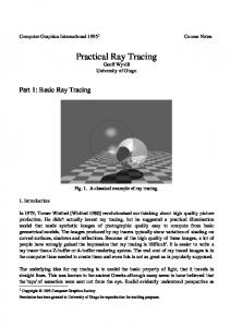
Chapter 1 Radiation If the word radiation comes up, mainly people think just of nuclear radiation. And it is sometimes hard to explain, that nuclear radiation covers only a small range of the entire concept of radiation. Figure 1.1 shows the full spectrum that belongs to radiation and outlines the small fraction of nuclear radiation. A short introduction in the usual bands and there reasons for the differentiation should be given. Radiation is the remote exchange of energy from one body to another. The process does not require a medium for the transport. So particles and photons are traveling on more or less straight lines through space. The consequence radiation causes by the arrival at a body, depends mostly on the carried energy. For instance, small quantities of transfered energy might have little effect, whereas high energy transfer can lead to dissolution of a compound or to mutations. Radiation can be subdivided by energy content as well as the driving mechanism for an energy transfer. Ionization is a charge state change of an atom or molecule to an ion, by adding or removing of charged particles. If radiation has the necessary amount of energy to ionize atoms or molecules, it is called ionizing radiation, opposed to non-ionizing radiation. Typical types of ionizing radiation are alpha, beta or gamma radiation. The energy exchange forms with particles for alpha and beta radiation, whereas with gamma radiation electromagnetic waves

Figure 1.1: The electromagnetic wave spectrum is outlined with the temperature at which it is typically emitted. (Source: Wikipedia.)

3

4

CHAPTER 1. RADIATION

are sent out. With the wavelength λ, speed of light in vacuum c and the Planck’s constant h, the energy S of a photon, electromagnetic wave, can be derived, S=

c·h =ν·h . λ

(1.1)

Thus the frequency ν is given with the speed of light divided by the wavelength. Ionization is only possible for a range of small wavelengths. Non-ionizing radiation is usually electromagnetic radiation with a lower energy content as required for ionization. Still, sufficient energy for changing the inner energy of the target can be provided. The total electromagnetic spectrum expands from ionizing gamma rays of less than 10 pm, to visible light (380 nm -780 nm), thermal radiation (0.78 m -1 m), to finally radio waves of several hundred thousand meters. This work mostly deals with thermal radiation relevant to heat transfer. With a relative large wavelength, thermal radiation is non ionizing. Interference effects, that are only important at very small length scales neglected here.

1.1

Thermal radiation

The guiding book for the theoretical work was from Siegel and Howell [1]. It can be said that, all necessary information for calculation of radiative heat transfer is given in this book. The most formulas and explications are described in an analogical manner. Also the book from Petty [2] or the lecture script [3] can be recommended, for basic understanding of radiation phenomena. Heat transfer consists of three major regimes; conduction, convection and radiation. All describe a mechanism of energy transport due to temperature differences. Often they occur in combination. Conduction is the thermal energy transfer due to small scale interactions of two participants, e.g. atoms, molecules and electrons. Hence for conduction it is essential that the participating media of the heat transfer are physically connected. When the thermal energy flow is caused by a macroscopic, joined movement of atoms or molecules, one speaks of convection. Is the convection due to buoyancy, the thermal process is called free convection or natural convection. Otherwise, the atoms or molecules (and thereby the thermal energy) are carried by a forced flow, the process is called forced convection. While conduction and convection depend on local derivatives and a physical medium with non-zero density is necessary, whereas thermal radiation also proceeds though vacuum. The nonlinear driving term for radiation is the temperature to the fourth power.

1.1.1

Blackbody radiation

The impact of thermal radiation on walls is not only conditioned by surface properties, but as well on the material under the surface. In general incident radiation can be reflected, transmitted or absorbed. The not reflected fraction of the incident radiation, which is not absorbed, will be transmitted. An opaque material transmits no incident radiation. Hence the radiation properties of an opaque body can be reduced to the surface of the body. This simplification is met by most solid materials.

5


An opaque body with a non-reflecting surface is named backbody. A blackbody absorbs all incident radiation, since no energy is reflected or transmitted. In stationary thermal equilibrium, the equal amount of energy absorbed must be emitted. Otherwise the temperature would change, as radiation is the only possibility of thermal energy exchange in vacuum. That a body always radiates and absorbs even in thermal equilibrium is known as Prevost’s law. Thermal radiation in vacuum is only a function of the body’s temperature. The second law of thermodynamics implies that a positive net amount of energy transfered from a body with lower surface temperature to a body with higher surface temperature is usually denied. Hence, the ratio of temperature to the total energy flux caused by radiation is also monotonically increasing with temperature. The quantification of radiation is commonly stated in terms of the amount of energy per time and area, which is called intensity. While the spectral intensity iλb of a blackbody is dependent on the wavelength, the total intensity ib is given as integral of the radiation over all wavelengths, Z ∞

ib =

(1.2)

iλb (λ) dλ .

0

The subscript b denotes that the quantity is associated with a blackbody. The second subscript λ is the dependence on the wavelength. Geometric context

Assuming a solid angle dω on a unit sphere. The surface element dA is located at the center of the sphere. The radiating surface element dA′ has a face-normal n. The slope of n to the normal of the surface dA is described by the polar angle θ, while azimuthal rotation is determined by the angle ϕ. In a cartesian coordinate system, a surface element dA′ on the unit sphere, given by dω,

Z

dω θ dAp

iλb

n dA′ Y

dA ϕ

r

X Figure 1.2: Influence of the angular position of two surfaces on the radiation.

6


can be parameterized on using the angles ϕ and θ [3],   sin(θ) cos(ϕ) n(θ, ϕ) =  sin(θ) sin(ϕ)  , (1.3) cos(θ)     cos(θ) cos(ϕ) − sin(θ) sin(ϕ) ∂n ∂n dθ dϕ =  cos(θ) sin(ϕ)  ×  sin(θ) cos(ϕ)  dθ dϕ = sin(θ) dθ dϕ . × dω = ∂θ ∂ϕ − sin(θ) 0 (1.4) Isothermal and isotropic blackbody radiation at an infinitesimal wavelength band dλ is emitted by the surface element dA′ . Thereby, the incident energy flux density Q˙ λ,i dλ on the surface element dA in direction of the normal vector n is iλb,n dλdω. The impacting radiation intensity at the surface dA depends on the mutual viewing angles. The intensity is uniformly emitted from dA′ into a hemisphere over this surface element (see figure 1.3 on the left). The total transfered energy arriving at dA is correlated to the projected area of the dA onto this hemisphere. To derive the total transfered energy, the intensity is integrated over the area matching solid angle dω. Obviously, iλb,n dAp = . 4π iλb

(1.5)

For the transfered intensity, not the total area of the dA is relevant, but the projected area of the surface element dA, denoted by the subscript p. The projected surface can be estimated with dA · cos θ, for an infinite small surface element. The radiation intensity is linked to the distance of the surfaces, which is described in this case by the radius. Due to conservation of energy, it must decay with the square of the distance r. As well, this relation can be deduced from the mutual view. The arriving intensity fraction at dAp was formed with using the total surface area of the unit hemisphere 4π. For the surface area of a general hemisphere is 4πr 2. For the calculating the fraction Ap /4πr 2 the concern of 1/r 2 is explained. Summarized gives this, dλ cos(θ)dλ ′ Q˙ λ,i (λ, θ, ϕ) = iλb (λ) cos(θ) 2 dA′ dAp = iλb,n (λ) dA dA . r r2

(1.6)

Lambert’s cosine Law The emissive spectral power eλb is the emitted energy per unit time from a blackbody. In contrast to the intensity iλb , the emissive spectral power is not originating from the projected surface, eλb (λ, θ) = iλb (λ) cos(θ) .

(1.7)

This relation (1.7) is known as Lambert’s cosine law. The emissive power is proportional to the physical amount of transfered energy in a certain direction θ. Specifying the content of emitted radiation is the more meaningful quantity compared to the intensity. The hemispherical spectral emissive power of a blackbody at a certain wavelength is related to the incident radiation. This is a quantity represents the total possible transfered energy. While using equation (1.4), for the emitting surface element dA′ results, Z 2π Z π/2 eλb (λ)dλ = iλb (λ)dλ cos θ sin θ dθdϕ = iλb (λ)dλπ . (1.8) ϕ=0

θ=0

7

CHAPTER 1. RADIATION θ

eλb or eb

iλb or ib

111111111111111111111 000000000000000000000 000000000000000000000 111111111111111111111

θ

111111111111 000000000000 000000000000 111111111111

Figure 1.3: The connection between the intensity iλb (left) and the emissive power eλb (right) is given by the Labert’s cosine law.

Planck’s Law The quantification of the emissive spectral power at each wavelength of the blackbody spectrum at an absolute temperature T is given [4] as, eλb (λ, T ) = πiλb (λ, T ) =

2πhc2 λ5 (ehc/λkB T − 1)

(1.9)

.

Hemispherical sp ectral emissiv p ower [e λb]=W/(mm 2 · µm)

While h is the Planck’s constant and kB denotes the Bolzmann constant. The wavelength λ and the frequency ν are connected, by the relation λ = c/ν and dλ = −(c/ν 2 )dν. The wavelength can change at the interface from one medium to another, whereas the frequency remains constant. 5500 K 5000 K 4500 K 4000 K 3000 K λ max

60

50

40

30

20

10

0

0.5

1

1.5

2

Wavelength [λ]=µm

Figure 1.4: The hemispherical spectral emissive power of a blackbody drafted over the wavelength λ. The correlation of temperature T and the maximum power density is indicated by λmax . For a blackbody with a temperature ∼ 5500 K like the sun, the maximum of the hemispherical spectral emissive power in the visible light band. The visible light band is indicated by the orange dashed lines.

Planck’s law is also applicable for media other than vacuum, if the associated wave propagation speed of the medium in equation (1.9) is taken into account. This is done by dividing the speed of light with the refraction index n = c/¯ c (explained in section 1.1.3).

8


The dependence of the hemispherical spectral emissive power, the wavelength and the temperature is shown in fig. 1.4. The higher the temperature the stronger is the total hemispherical spectral emissive power. It is note able that the maximum of hemispherical spectral emissive power moves to a lower wavelength range with higher temperature. The visible range of electromagnetic waves for humans is between 380 - 780 nm is only reached at high temperatures. Only for higher temperatures than the Draper point at 798 K the emission of a surface is visible for humans. The Planck’s law relies on the temperature T and the wavelength λ. To receive a simpler relation, a formulation with just one combined variable λT is favored, π iλb (λ, T ) 2πhc2 eλb (λ, T ) = = . T5 T5 (λT )5 (ehc/λkB T − 1)

(1.10)

If ehc/λkB T is large compared to one, the approximation is called Wien’s formula 2hc2 iλb (λ, T ) = . T5 (λT )5 ehc/λkB T

(1.11)

These equations facilitate the calculation of the wavelength λmax for which the blackbody intensity i is maximal for a certain temperature T . Equation 1.10 is differentiated with respect to λT and the left side is set to zero. The solution turns out as a simple constant, λmax T = 2.898

(1.12)

and is known as Wien’s Displacement Law . The Stefan-Bolzmann Law uses Planck’s law 1.9 to obtain another formulation for the total blackbody intensity ib by integrating over all wavelengths of the spectral intensity iλb , Z ∞ Z ∞ 2hc2 2k 4 π 5 T 4 T4 ib = iλb (λ) dλ = dλ = · = σ · , (1.13) λ5 (ehc/λkB T − 1) 15h3 c2 π π 0 0 where constant σ is the Stefan-Bolzmann constant. The hemispherical total emissive power eb can be described using of the total intensity ib , Z ∞ Z ∞ eb = eλb (λ)dλ = πiλb (λ)dλ = πib = σT 4 . (1.14) 0

0

The emissive power of a blackbody in a certain wavelength interval [λ1 , λ2 ] is of interest for segregated bandwidth calculations. It is usually expressed as fraction Fλ1 →λ2 of the total emissive power, R λ2 Z λ2 Z λ2 e (λ)dλ 1 π λ1 λb = Fλ1 →λ2 = R ∞ eλb (λ)dλ = iλb (λ)dλ . (1.15) σT 4 λ1 σT 4 λ1 eλb (λ)dλ 0

Here the benefit of using just one combined variable becomes clear. If only one variable λT is used, the shape of the function stays the same. So the band integration is treated out with two integrals from the lower bound zero two the upper bounds λ2 T and λ1 T , which are subtracted from each other, Z λ2 T Z λ1 T eλb (λ) 1 eλb (λ) d(λT ) − d(λT ) = F0→λ2 T − F0→λ1 T . Fλ1 →λ2 = Fλ1 T →λ2 T = σ 0 T5 T5 0 (1.16)

9

CHAPTER 1. RADIATION For integrating the partition F0→λT , series expansion is formed, Z ∞ 2 3 3CλT 15 X e−jCλT 6CλT 6 15 CλT CλT 3 CλT + dCλT = 4 + 2 + 3 , F0→λT = 1 − 4 π 0 eCλT − 1 π j=1 j j j j

(1.17) where CλT = hc/kB λT . Hence the fraction F0→λT gives the percentage of the hemispherical total emissive power for a certain wavelength and temperature. An interesting fact can be noticed, a quarter of the intensity is situated below the wavelength λmax .

1.1.2

Nonblack Opaque Surfaces

A blackbody emits and absorbs the maximum amount of energy. However, a real body has a grey surface. The emissivity ελ gives the ratio of the emitted spectral energy density of a real body compared to a blackbody. The absorptivity αλ can be equally defined as absorption fraction of a real body compared to a blackbody. The emitted energy flux density Q˙ λ,e per wavelength emitted from a certain surface A at temperature TA in a solid angle dω can be written as Q˙ λ,e (λ, θ, ϕ, TA )dλ = iλ (λ, θ, ϕ, TA ) cos θdλdAdω .

(1.18)

For a blackbody intensity iλb (λ, TA ) the directional dependence vanishes. Hence,the emitted energy flux density Q˙ λb per unity time and wavelength for a blackbody is Q˙ λb (λ, θ, TA )dλ = iλb (λ, TA ) cos θdλdAdω .

(1.19)

The subscript e can be dropped, since a blackbody emits as much as it absorbs. The surface emissivity ε expresses as ελ (λ, θ, ϕ, TA ) =

Q˙ λ,e (λ, θ, ϕ, TA )dλ . Q˙ λb (λ, θ, TA )dλ

(1.20)

The fraction of the energy flux density Q˙ λ,a absorbed by a real surface compared to the incident energy flux density Q˙ λ,i defines the absorptivity α, αλ (λ, θ, ϕ, TA ) =

Q˙ λ,a (λ, θ, ϕ, TA )dλ . Q˙ λb,i (λ, θ, ϕ)dλ

(1.21)

The incident radiation is deposited in a layer under the surface. For an opaque surface, the radiation is completely absorbed in the material and does not get through the body as transmitted energy. Nevertheless, the here defined emissivity and absorptivity thought of as surface properties. They depend on the wavelength the surface temperature and the incident angle. Hence, the quantities can vary in a complex manner. It is also difficult to measure emissivity and absorptivity with respect to all dependencies for a material. Therefore, simplified model assumptions are often made, such as constant values for a certain dependency. Kirchhoff ’s Law proposes correspondences between emissivity and absorptivity under some assumptions. Consider a surface element dA surrounded by an isothermal black environment and hit by an isotropic intensity of energy iλb (λ, TA ). The amount of absorbed and emitted energy is usually considered identical, ελ (λ, θ, ϕ, TA ) = αλ (λ, θ, ϕ, TA ) .

(1.22)

10


The part of incident radiation energy that is not absorbed at a non-black opaque surface has to be reflected. The challenge with calculating reflectivity is that is does not only depend on one single direction. It relies on the orientation to the surface from which the radiation is coming from as well as the direction in which the beam is reflected. Therefore, reflectivity is a bidirectional quantity. The incident intensity iλ,i (λ, θ, ϕ) is either absorbed or reflected in a direction (θr , ϕr ). Hence the reflected intensity iλ,r (λ, θr , ϕr , θ, ϕ, TA ) is only the intensity from (θ, ϕ) thrown back into the direction (θr , ϕr ). The incoming energy flux density Q˙ λ,i onto the surface element dA with temperature TA can be written as Q˙ λ,i (λ, θ, ϕ)dλ = iλ,i (λ, θ, ϕ) cos θdω . dλdA

(1.23)

The reflectivity ρλ (λ, θr , ϕr , θ, ϕ, TA ) can be therefore defined as ratio of the reflected to the incoming intensity, ρλ (λ, θr , ϕr , θ, ϕ, TA ) =

iλ,r (λ, θr , ϕr , θ, ϕ, TA ) . iλ,i (λ, θ, ϕ) cos θdω

(1.24)

Reflectivity is symmetric for the same incident and reflection angles, ρ(λ, θ, ϕ, θ′ , ϕ′ , TA ) = ρ(λ, θ′ , ϕ′ , θ, ϕ, TA ) .

(1.25)

The arriving energy at a nonblack opaque surface is divided into reflected or absorbed parts. For continuity reasons this can be stated as, αλ (λ, θ, ϕ, TA ) + ρλ (λ, θ, ϕ, TA ) = 1 ,

(1.26)

and by Kirchhoff’s law also, ελ (λ, θ, ϕ, TA ) + ρλ (λ, θ, ϕ, TA ) = 1 .

(1.27)

Since the absorptivity and emissivity depend on the surface temperature, also the reflectivity has to depend on it. As special assumptions for wall reflection behavior diffuse surfaces and gray surfaces should be mentioned. Diffuse reflection means that the energy is redirected without any directional preferences. In their case, reflection is not a bidirectional quantity any more, which simplifies computation. Gray walls exhibit reflections independent of the wavelength and therefore also absorption and emission must be independent of the wavelength.

1.1.3

Electromagnetic Theory

The electromagnetic theory, based on Maxwell’s equations, describes the interaction between electric and magnetic fields. Most phenomena of light or radiative heat transport can be described with it, since they consist of traveling electromagnetic waves. Also predictions for the absorptivity, emissivity and reflectivity can be deduced. Maxwell’s Equations The behavior of electromagnetic waves traveling through a material can be characterized by Maxwell’s equations. The magnetic field strength H and the electric field E in an isotropic,

11

CHAPTER 1. RADIATION neutral medium are thereby, E ∂E + , ∂t σE ∂H , ∇×E = µ ∂t ∇·H =0 , ∇·E = 0 ,

(1.28)

∇ × H = ε0

(1.29) (1.30) (1.31)

where t is the time, ε0 the permittivity, σE is the electrical resistivity and µ is the magnetic permeability. For first investigations of the propagation of the radiant wave, a homogeneous, isotropic medium with a high electrical resistivity like vacuum is assumed. This should simplify calculation, because on that score the term E /σE can be neglected. The wave is assumed constant in Y , Z. With this assumptions, the magnetic field H or either the electric field E can be eliminated in the simplified Maxwell’s equations. They form to wave equations of the propagation of E , ∂ 2 EY ∂ 2 EY ∂ 2 EZ ∂ 2 EZ µε0 = µε = . (1.32) 0 ∂t2 ∂X 2 ∂t2 ∂X 2 The solution for EY can be expressed by two functions f and g, which represent a right and a left running wave in X direction, t t EY = f X − √ +g X + √ . (1.33) µε0 µε0 √ The propagation speed of the wave front c can be read out as dX/dt = 1/ µε0 . By superposition of fixed spectral waves in a Fourier series, the waveform f can be obtained as well. The waveform propagation in time, traveling with wave speed through a medium, can be written as, bY eiωrad (t− Xc¯ ) = E bY eiωrad (t− nc X ) , EY = E

(1.34)

bY is the magnitude of EY and ωrad = 2πc/λ is the angular frequency of the wave where E with the wavelength λ in vacuum. The wave front speed c¯ is normally expressed by with the refractive index n, which is the ratio of the wave propagation speed c in vacuum to the wave propagation speed in the medium c¯. If the previous simplification of neglecting the term E /σE is now considered relevant the Maxwell’s equations result in, µε0

∂ 2 EY µ ∂EY ∂ 2 EY = − ∂t2 ∂X 2 σE ∂t

µε0

∂ 2 EZ ∂ 2 EZ µ ∂EY = − , ∂t2 ∂X 2 σE ∂t

(1.35)

with solution of the form, bY eiωrad (t− c¯ ) e− EY = E X

ωrad Kλ X c

bY eiωrad [t−(n−iKλ ) c ] . =E X

(1.36)

Kλ is called the extinction coefficient, which can be formally interpreted as complex refraction index n ¯ = n−iKλ . Inserting the solution 1.36 into 1.35 and split into the real and imaginary part, defines the refraction index n and the extinction coefficient, n2 − Kλ2 = µε0c2

,

nKλ =

µλc . 4πσE

(1.37)

12


The energy S of an electromagnetic wave can be calculated as cross product of electric and magnetic intensities, which can be obtained with the Maxwell’s equations and gives, n ¯ (1.38) |S | = |E |2 . µc The volumetric absorption a of a medium is the energy decay per unit length, which inserting 1.36 into 1.38, 4πKλ a(λ) = . (1.39) λ Fresnel’s Equations For contemplation of reflection and refraction at an interface between two perfect dialects materials, only the real part of the energy wave in y direction is considered. Since the waveform can be described with equation (1.34) and the complex exponential function can be split into real and imaginary part by the real cosine and imaginary sinus functions. The wave is polarized. The incident electric field can be divided into a part parallel and normal to the surface. The usual way to describe the partition is to use the sinus and cosine of the angel θ, which is the tilt of the incoming wave direction to the normal vector of the surface. For the reflected direction an angle θr and for the refracted intensity an angle Ψ can be defined, for which the intensities are separated to a parallel and normal component. With the boundary condition at the interface, that the sum of the incident and the reflected field must be equal the refracted polarized intensity, the relation n1 sin θ = n1 sin θr = n2 sin Ψ

(1.40)

can be obtained, which hence also θ = θr . The relation between the refraction indices is known as Snell’s law , n1 sin Ψ . (1.41) = sin θ n2 This boundary condition must also hold for the magnetic field. Parallel to the surface the transition must be continuous. Hence, the incident plus the reflected results the reflected magnetic intensity. The electric field vector is perpendicular to the magnetic intensity vector. Thereby the relation between the reflected and incident intensity amplitude polarized parallel k to the incident plane can be given through the Fresnel’s equations, bkr E n2 cos θ − n1 cos Ψ =− . bki n2 cos θ + n1 cos Ψ E

(1.42)

As well as for polarization perpendicular ⊥ to the incident plane, b⊥r n2 cos Ψ − n1 cos θ E =− . (1.43) b⊥i n2 cos Ψ + n1 cos θ E The ratio of the reflected to incident intensities gives the reflectivity ρ. The energy of a wave is correlated to the square of the field strength, !2 !2 bkr b E E⊥r ρλ⊥ (λ, θ, ϕ) = . (1.44) ρλk (λ, θ, ϕ) = b b⊥i Eki E

For in polarized incident radiation the reflexion coefficient is given by the average of the both, ρλk + ρλ⊥ . (1.45) ρλ (λ, θ) = 2

13


1.1.4

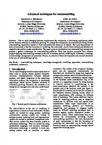
Spectral dependency

Material properties like absorptivity, emissivity or reflectivity normally vary with the wavelength. These spectral effect can be very large, e.g. the volumetric absorption and emission in carbon dioxide and water vapor, or the gas mixtures in combustion chambers. Another example is the difference of the solar irradiance outside the earth atmosphere and on the ground. The solar spectrum at high altitude has nearly a blackbody distribution with a temperature of approximately 5500 K - 5800 K. Many spectral bands are filtered by different gases, as it can be seen in figure 1.5. The energy of an electromagnetic wave was given in equation (1.1). However, due to quantum mechanics reasons the energy transported as electromagnetic wave is a discrete quantity. Atoms or molecules can exchange energy as vibrational or rotational but again discrete states. This results in lines in the spectral space. Also the dependence of the material properties on the wavelength can thereby closed. For practical reasons, the complex spectral dependence is replaced by bands. One model is the narrow-band model, where the integration is done over all lines to receive the entire contribution. Whereas line by line calculation has an enormous expense, the lines are modeled with structure of a narrow spectral band. The spectral interval covers only a fraction of the complete vibration rotation band. The spectral properties of the line shapes, widths and spacing are used for this computation. The wide-band model captures the total vibration rotation band. This means that not every single wavelength is calculated separately. The focus of both models are the global properties. The spectral attributes must be estimated over the band range. The simplest non gray band model is the weighted sum of gray gases model (WSGG) . The volumetric emissivity ǫ is estimated by a weighted sum over N species and the beam length ∆l, N X ǫ(l) = wj (1 − e−aj ∆l ) , (1.46)

Sp ectral irradiance W/(m 2 µm)

j=1

Extraterrestrial spectrum 2000

Global spectrum at sea level Direct spectrum at sea level Energy distribution for a blackbo dy at 5500 K

1500 O3 1000

500 O3 O2 0

0.5

H 2O 1

H 2O

H 2O 1.5

H 2O 2

2.5

Wavelength [λ] = µm

Figure 1.5: The spectral irradiance of the sun [5](ASTM G-173-03 International standard ISO 9845-1,1992). The gases accountable for the band absorption are indicated.

14


with the weight wj and the absorption coefficient aj of the gray gas. The weight is usually constructed, corresponding to the molar mass fraction of the entire medium. But, homogenous medium in the calculation domain is required, since the weight is not defined as local quantity. Hence, only constant absorption coefficients are allowed. This is hardly the case for combustion problems, still computational speed can require this model. A related enhancement is the spectral line weighted sum of gray gases model (SLWSGG). There the integration is done over fixed non overlapping wavelength intervals ∆λ. The weighted sum given in equation (1.46) is used, but the weights are modeled differently. The basic thought is similar to the idea presented in chapter, but uses a cumulative distribution function F∆λ . The weight w dependent on the wavelength interval ∆λ, the position x of the center of a volumetric mesh cell (see section 3.3.1), the local temperature Tb and molar fraction ξ for each non gray gas, Z π X F∆λ (x , Tb , ξj ) = ib (Tb , λ)dλ . (1.47) σTb4 j ∆λ (x ,ξj ) Thereby the weight can be written as, wk = F∆λ (x k+1 , Tb , ξj ) − F∆λ (x k , Tb , ξj ) .

(1.48)

Thus with the weight the volumetric emissivity and further the emitted intensity can be calculated. In literature, SLWSGG is often considered as the best compromise between accuracy and computational effort. It can provide a higher functionality then WSGG. While line by line methods are more precise, the calculation effort is large.

1.1.5

Scattering

The redirection of radiation due to the interaction with particles or molecules in a medium is understood as scattering. The change of intensity idλ in a certain direction along a distance l is given by Bouguer’s law, Rl ′ (1.49) iλ (l) = iλ (0)e− 0 Kλ dl . Kλ is the spectral extinction coefficient of the medium. The variation of the directional intensity depends on the volumetric absorption aλ and the scattering coefficient σs ; Kλ (λ, T, P ) = aλ (λ, T, P ) + σsλ (λ, T, P ) .

(1.50)

Scattering takes place as interaction with particles or molecules. The scattering coefficient is conditioned to the pressure P in the volume, which is usually correlated to the number of particles in the volume. Where Npm is the number of particles or molecules per unit volume. The spectral scattering cross section Ds,λ is the area of a particle or molecule a beam faces on the way through the medium, which can be different from the real physical cross section. Therefore the scattering efficiency factor Qs gives the proportion of Ds,λ to the geometric projected area Dp of the particle. Then the scattering coefficient σsλ can be defined as, σsλ = Ds,λNpm = Dp Qs Npm .

(1.51)

Similar to the scattering efficiency factor, the absorption efficiency factor Qa can be defined, for quantification of absorbance of the particles or molecules.

15


Usually the integral of the extinction coefficient Kλ over path length l is called opacity κλ . If κλ ≪ 1 the medium is treated as optical thin, while if κλ ≫ 1 the medium is optical thick. In this contents, the albedo Ω is defined and occurs often in scattering specifications. It states the importance of scattering compared to absorption, Ω=

σsλ (λ, T, P ) . aλ (λ, T, P ) + σsλ (λ, T, P )

(1.52)

Is the energy, and hence the frequency of the electromagnetic wave or photon, unchanged during scattering, the process is call elastic opposed to in elastic scattering. Anisotropic scattering signifies that the photon is deflected in a not regular manner, oppositional states isotropic scattering. For anisotropic scattering, the directional distribution is given by a phase function Φ. Different scattering descriptions have individual phase functions. To categorize effects of scattering of a particle, a dimensionless parameter Γ = πd/λ is useful, where d is the diameter of the particle. It turns out, that for Γ > 5 can be treated as reflexion on large spheres. For Γ < 0.3 the deflection effect can be handled satisfactory by Rayleigh scattering. In the range between, a more complex description of the process is needed and known as Mie scattering. Rayleigh Scattering is very important for the humans emotional state, since this scattering effect colors the sky blue and is responsible for the light effects at sunset. This effect occurs when the particles size is small compared to the wavelength. The scattering cross section Ds,λ [6] shows a strong dependence of the wavelength λ, Ds,λ

2 π 5 d6 = 3 λ4

n2 − 1 n2 + 2

2

.

(1.53)

Where d is the diameter of the particle and n is the refraction index. Thus, Rayleigh scattering is more intense for electromagnetic waves with short wavelengths. The phase function Φ for Rayleigh scattering is anisotropic and only a function of the deflection angle θs , 3 Φ(θs ) = (1 + cos2 θs ) . (1.54) 4 The deflection angle is defined zero in the original direction of the radiation. Mie Scattering is used when the particle is to large for Rayleigh scattering and to small for sphere collision [7]. Strong polarization effects can occur and therefore the complex refractive index n ¯ is used. Also the phase functions are rather simple and a general function for Mie scattering does not exist. The scattering cross section Ds,λ is written as an expansion, Ds,λ

2 2 3 π 2 d2 n ¯ −1 ¯2 − 2 2 π 5 d6 n . 1 + + . . . = 3 λ4 n ¯2 + 2 5 λ2 n ¯2 + 2

(1.55)

Scattering on large spheres depends on many factors [8]. The real shape and surface behavior of the particle surface becomes important. Therefore no simple general relations can be given.

16


1.1.6

Radiation transport equation

In this section, the segregated theory is drawn together into the governing equation of radiative heat transfer. The change of intensity of an electromagnetic wave per traveled length is described by the radiation transport equation. The radiation transport equation can be formed as an energy balancing equation. Electromagnetic waves are assumed to travel with a certain direction on straight lines thought a homogenous medium. The intensity i of the wave will depend on time t and on the covered distance l. Hence intensity variation can be written as, di ∂i 1 ∂i = + dl ∂l c¯ ∂t

c¯ =

∂t . ∂X

(1.56)

For treating thermal heat transfer, the time derivative can be neglected. Due to the reason that the wave propagation speed is large, the influence of this term is small. So the time derivative is of relevance in sort time scales. Normal observation periods for thermal applications are much larger than 1/t. As mentioned in section 1.1.3 the electromagnetic wave loses intensity to the medium, while passing through it. This is modeled trough to volumetric absorptivity a, see 1.39. The medium can partially reemit the absorbed energy, to stay in equilibrium state. Further, a wave can be scattered or redirected by hitting some particle, see section 1.1.5. Thus the directional intensity carried by the initial beam along the initial heading direction decreases due to scattering. Nevertheless, other beams coming from different directions are scattered in that heading direction of the initial beam,leading to a secondary growth of the intensity. The corresponding mathematical expression of that phenomena is called the inscattering term. For many numerical models, it is a problematic term, since the different direction ω ′ makes the treatment sophisticated. Some simplifications are normally made, e.g. the phase function Φ characterizing the preferred direction in which scattering occurs. The modeling of the in-scattering term will be outlined in chapter 2. So the variation of intensity i in direction ω can be denoted as, Z diλ (ω, λ) σs Φ(θs )iλ (ω ′ , λ) dω ′ . (1.57) = −(a + σs ) iλ (ω, λ) + a ib (T ) + dl 4π 4π

The equation is valid for individual wavelengths and must be integrated over all wavelength bands. The negative, first term on the right side, represents the losses due to out scattering and volumetric absorption. The second contributes to the intensity by blackbody emission of the medium, which is given by the fourth power of the temperature of the gas and the Stefan-Bolzmann constant σ. The medium is considered in equilibrium state, therefore Kirchhoff’s law can be applied and the volumetric emissivity can be replaced by the volumetric absorptivity. For complex gases or mixtures often a band model, see section 1.1.4, is necessary, to determine the actual volumetric emissivity. The last term on the right side, is the in-scattering term. Boundary Conditions For solving differential equations, boundary conditions are required. For non-participating media, they are only relevant on active surfaces. In the historically early stages of graphical ray tracing only wall interactions where considered. At walls, energy conversation must hold. For a thermodynamic equilibrium state, the total outgoing intensity io and the total incident intensity ii for a fractional area dA must

17


dA

ω dA′′

x

n

n′′

||x − x′ ||2 n

x′′

ω ′′

′

ω′

x′ dA′ Figure 1.6: Directional relations between the surface elements.

be equal. The incoming intensity can be absorbed, reflected and transmitted at the target surface. A thermodynamic equilibrium state is assumed and according to the Kirchhoff’s law, the absorbed must equal the emitted intensity. Thus, the incident intensity is the sum of the emitted intensity ie , the reflected intensity ir and the transmitted intensity it , ii = io = ie + ir + it .

(1.58)

The position x lies at the observed fraction area dA and the outgoing intensity is emitted in direction ω. Further, x ′ is the position of the fractional area dA′ , where the incoming intensity was emitted and the direction ω ′ states the geometric directional relation of the to surfaces elements. The incoming energy from a surface element dA′′ hitting the surface element dA′ at x ′ is always thrown back by reflection into the previous medium. The surface normal vector n ′ of dA′ is considered pointing into the medium. Hence, the incident intensity comes from a positive hemisphere H+ above the surface element and the reflected intensity leaves again in the same hemisphere. Whereas for the transmitted energy leaves through the negative hemisphere H− under the surface element. Hence reflection and transmission are, opposed to the emitted intensity, bidirectional quantities, as mentioned in section 1.1.2. They depend on the incident direction and on the outgoing direction. Therefore they need to be integrated over the according hemisphere, where the bidirectional dependence is stated by mr for the reflection and mt for transmission, Z mr (x , ω ′ , ω, λ, t)ii (x , ω ′ , λ, t)(−ω ′ · n)dω′ + ii (x , ω, λ, t) = io (x , ω, λ, t) = ie (x , ω, λ, t) + ZH+ mt (x , ω ′ , ω, λ, t)ii (x , ω ′ , λ, t)(−ω ′ · n)dω′ . + H−

(1.59)

Thus the transferred intensity ii per unit time t per unit area of source dA′ and per area ˙ of target dA gives the energy flux density of radiation Q, ˙ Q(λ, t) = ii (x , x ′ , λ, t) dt dA dA′ .

(1.60)

The total incident intensity ii hitting dA from dA′ consists of the emitted intensity from dA′ in direction ω ′ and intensity emitted from dA′′ back-reflected over the irradiated dA′ , as

18


illustrated in figure 1.59. The emitted intensity is derived with the emissive power e of the surface element with respect of the mutual view of the surface elements. Hence, The dependence of the transferred intensity from the surface element dA′ to the surface element dA is known. The geometric factor form is given as, cos ω ′ dω ′ = (−ω ′ · n) dω ′ =

cos ω cos ω ′ ′ dA ||x − x ′ ||2

(1.61)

and be back inserted into equation (1.59). The visibility of the two faces must be taken into account, which is normally done by multiplying the geometrical factor with a Dirac delta function. For all surface elements equation (1.59) can be written in matrix form, i = G eb + G M i ,

(1.62)

where i states the incident intensity in vector form, G is the matrix of geometric view factors, e b the emissive power vector and M is the linear matrix operator representing the integral of bidirectional relation. Finally, equation (1.62) only depends on the source terms that are considered as boundary conditions. However, this method lacks any volumetric interactions.

Chapter 2 Numerical models for thermal radiation Thermal radiation is often dependent on complicated boundary conditions. Hence, calculations can seldom be done analytically. Thus the solution must be achieved numerically. For thermal radiation, several models have been developed. They differ in complexity, specific operational area and their numerical effort. Each model relies on different assumptions and has therefore advantages and disadvantages. They should be known for the right choice of radiation model. An overview of commonly used methods is given in the appendix A, while a comparison of the radiation models for an test case is described in section 4.1.2. The most common numerical models can be found in [1], which gives all the necessary information for implementation of most methods. In the work of Guillem Colomer Rey [9] two numerical methods for thermal radiation are shown more detailed, the radiosity-irradiosity method and the discrete ordinates method. For some problems conduction, convection and radiation need to be calculated together. For instance, the phenomena could depend on each other or they are similarly influential for the solution, that none of them can be neglected. Usually numerical programs for simulation of fluid flow and heat transfer provide a couple of models for thermal radiation simulation. Commonly used software simulation tools are e.g. OpenFOAM or Fluent. Some minor documentation can be found in the manuals [10] and [11].

2.1

Ray tracing

There are many fields in science, that use tracing methods. Of course, they apply this method for different occasions and as a consequence these methods are related but not equal. Several operational areas for ray tracing are not obvious. For instance, ray tracing is also used in multi-body dynamics. The gravitational attraction let bodies interact with each other. The force, like the intensity of radiation, decays with the inverse squared distance. So modified radiation algorithms find usage in that area. Also the sound propagation in a theater or opera hall or the progression of a shock in a one-dimensional wave is calculated with ray methods. Hence, the definition of ray tracing varies a bit for each area of application. Ray tracing, in physical understanding, is a method to solve a problem by tracing the path of a particle or wave through space. In case of radiation, every particle or wave has characteristic properties, such as velocity, intensity or frequency. They can vary or change on the way through the system. This can be caused by volumetric absorption, reflection on surfaces, transmission or other physical reasons. However, the track of the particle or wave with all it’s properties form a ray. So with ray tracing a bundle of rays are sent into the 19

CHAPTER 2. NUMERICAL MODELS FOR THERMAL RADIATION

20

system. The mutual reaction is detected and result as solution of the problem. Tracing the ray from an illuminated face or image plane to the source, is called backward ray tracing and used for image generation. For graphic applications, the interest is the image plane not the distribution in the entire system. In contrast to that, thermal applications are interested in the full solution, on all surfaces as well as the volume. While starting a ray at the illuminated face, the physical attributes of the ray are not known yet. Once the ray attains his physical originator, they become defined. With them, the effect of the ray can be calculated. This is a costly procedure for the treatment of one ray. Still this method can be used to exploit the contiguity of starting and termination point and also for implicit formulations. For example view factors used in the surface to surface approach (see appendix A) can be evaluated with that strategy. Hence, the ray tracing is only preformed once and the expansive manner of creation is of little concern. In contrast, following the ray from the emitting source to an object that reacts with the ray, is called forward ray tracing or particle tracing. With the knowledge of the emitted intensity and direction the ray is traced in the physical direction. Thus physical interactions can be easily carried out. The aim is a realistic and physical correct solution. Therefore this method is preferred for further investigation in this work. Theoretically, ray tracing needs to evaluate all possible light paths. As there are an infinite number of those, an integration should be performed. Since there are different methods for this integration, ray tracing can thereby be classified. Monte Carlo integration is one possible summation method and the common choice. Ray tracing can be as well assorted in biased or unbiased methods. Roughly speaking, a bias is the error by a shifted mean value. A small bias is sometimes tolerated to get faster algorithms, but it is difficult to estimate the bias. The knowledge of the error size is required to guaranty a meaningful result. To achieve an accurate result, an unbiased method is superior for heat transfer applications. There has been done impressive work in computer graphics last years. New methods have been developed, like bidirectional path tracing [12] and photon tracing [13]. They combine forward and backward ray tracing. Those methods facilitates the sampling on regions that are required for the picture generation. Areas, that are rarely illumined, are excluded from computation. This is of course done to save computing time and enable realtime image calculation. For heat transfer applications is not actable to neglect areas. So this method will not be applied in this work. There are some techniques, that describe the manner how rays should be emitted.

2.1.1

Markov chain

The Markov chain is very useful to describe a random processes, e.g. queueing [14]. There are several fundamental characteristics of a Markov chain, that are essential for some ray tracing methods using Monte Carlo integration. For that issue Markov chains will be discussed shortly. Proofs of this mathematical method are given in [15] and [16]. The latter has various appealing examples that facilitate comprehension and gives also a recommendable overview on statistics, while [15] focuses on the stability of Markov chains. A process starts at an arbitrary state sj of all possible states and moves continuously to another state sj ′ of all possible states. Every move from a state to another is realized with a certain transition probability pjj ′ ∈ [0, 1]. Every single movement or change of state is called step. The probability only depends on the current state, not on the state before. Such a process is called a Markov chain. The transition probabilities create element-wise the transition matrix P. So this matrix


21

gives a possibility map for the direction, into which the following step will be done. To calculate the new probability after a step, an initial probability vector s 0 is multiplied with the transition matrix P. For k steps the transition matrix needs to be taken by the power of the number of steps k, s (k) = Pk s 0 . (2.1) All possible steps are represented by one row of P. The sum of all probabilities moving from one state to any other state in a normalized transition matrix must be one. Normally the states are known and the converged transition matrix is required. In terms of ray tracing, the relation of states is made by rays. The transition probability pjj ′ between these states is then calculated. Absorbing Markov chains consist at least one absorbing state and this state is accessible from every other state. From an absorbing state it is not possible to leave, meaning the transition probability of this state is one. A non absorbing state is called transient. Hence, at an absorbing state the process or (e.g. ray tracing) a ray ends. If one absorbing state is reachable from every other state in the Markov chain, every process will be absorbed as the number of steps goes to infinity. Also of interest is the time or the number of steps, until an absorbing state is reached. For that reason, the transition matrix is reordered, so that the transient states come first. The matrix, without the rows and columns of the transient states, is denoted as V and the identity matrix as 1. The existing fundamental matrix is defined as (1 − V )−1 . The fundamental matrix can be determined though the expansion 1 + V + V 2 + · · · + V n . The elements give the number, a state sj ′ was selected from an initial state sj,0. The time t is a column vector, where the j th element correspond to the time, in which the state sj is absorbed. This vector can be simply calculated by the multiplication of the fundamental matrix with a column vector containing j elements with the value 1. Ergodic Markov chains signify that each state is reachable from any other state, possible using intermediate steps. Regular Markov chains are ergodic Markov chains and each state is reachable in exactly k steps, where k is a constant number. This can also be expressed as for some power k of the transition matrix P, the transition matrix Pk has only positive elements. For the convergence of a regular Markov chain, a limiting matrix W can be defined, W = lim Pk . k→∞

(2.2)

All rows w of the limiting matrix are equal. The elements of w are all positive and add in sum up to 1. Pk for a regular Markov chain converges to a Matrix with constant columns. Also w can be interpreted as left eigenvector of the transition matrix. As it is the goal of ray tracing to calculate the converged transition matrix P, also the vector w can be calculated instead. The essential theorem for Monte Carlo ray tracing is, that the unique defined probability vector w can be obtained, by starting a regular Markov chain, with an any desired probability vector p any , an after k → ∞ steps converged solution will be received, lim Pk p any = w .

k→∞

(2.3)

22


Ray tracing works, by emitting k random rays into the system and solving the interactions. The mathematical basis of ray tracing is solid, as long as it is made sure, that the process is a regular Markov chain.

2.1.2

Monte Carlo method

The Monte Carlo method is a mathematical stochastic method of performing an integration. This procedure is superior in multidimensional integrals or if the integration domain has a complicated shape, see [17], [12] and [18]. For normal Monte Carlo integration, random distributed samples are used for the estimation. In figure 2.1, samples for integration over a quarter of a unit circle shown, where the total samples are spread over a unit square. The probability of a hit into the quarter sphere relates to all hits, as the area of the quarter circle to the area of the enclosing square. Thus, the samples located in the quarter circle are counted and divided by the sum of the total number of samples N. This gives an approximation of the integral. The accuracy increases with the number of samples. An analytical specification for the boundary of the integration domain is not essential. After this introductory words the mathematic perspective shell be treated. Consider a function f (χ) and a probability density function p(χ) for a random (potentially multidimensional) sample point χj = [χ0 , . . . , χN ]. The expected value for a function is defined as Z hf (χ)i = f (χ)dη . (2.4) By computing the mean of the function f the Monte Carlo estimate, indicated by a tilde, is gained. This is done by summing the samples f (χj ), which are picked accordingly to a probability density function and divide by the total number of variables, N 1 X f (χj ) fÑ (χ) = . N j=1 p(χj )

(2.5)

Y

If the random variables originate from a uniform probability density function and are chosen

X

Figure 2.1: Integration over a quarter of a unit circle with the Monte Carlo method. The samples in the circle are colored black, whereas the samples apart from the circle are red.


23

independently, the form can be rewritten as, N 1 X ˜ f (χj ) . fN (χ) = N j=1

(2.6)

Since χ is a random variable, fÑ (χ) can also be comprehend as a random variable. Further is fÑ (χ) called the Monte Carlo estimator of the expectation value of f (χ). The solution can be made as exact, as desired with a certain large number of samples, lim P(|fÑ (χ) − hf (χ)i| ≥ ε) = 0 ,

N →∞

(2.7)

where P denotes the probability and ε is an arbitrary positive number. An essential observation is, that the Monte Carlo estimator is unbiased for the expectation value of f (χ). This can be concluded from, + * N N X 1 X 1 f (χj ) = hf (χj )i = hf (χ)i . (2.8) hfÑ (χ)i = N j=1 N j=1 The Monte Carlo estimator also shows a certain variance. Which can be simple computed; ! N N X 1 1 X hf (χ)2 i − hf (χ)i2 ˜ V ar(fN (χ)) = V ar f (χj ) = [f (χ) − hf (χ)i]2 p(χ) = . N j=1 N j=1 N

(2.9)

Finally, the expected value of Monte Carlo integration can be written, hf (χ)i =

2.1.3

Z

N 1 1 X . f (χj ) ± O √ f (χ)dη ≈ N j=1 N

(2.10)

Variance reduction

The absolute error of normal Monte Carlo integration decays with order of the square root of the number of samples. There are multiple variance reducing methods. These sampling methods are invented to achieve faster converge rate than O(N −1/2 ). A fast convergence rate is not the aim of a good estimator. The computational cost per sample is relevant. Hence, the efficiency of an estimator could be defined as, efficiency =

1 . variance · time

(2.11)

On that score, there exists methods for saving computational time by increasing the variance a bit. Some, relevant to heat transfer, are outlined. A good overview can be found in [12] and [17]. This methods are listed in the order in which manner samples are taken or chosen. First random point picking or fixed sampling for basic Monte Carlo integration is reviewed. Afterwards uniform and importance sample placement methods are described. The category of adaptive sample placement is mentioned. This procedure adjusts chosen samples and therefore they act in a complete different way.


24

Random Point Picking or fixed sampling is the naive application of coincidental sample selection. It is done without regarding the contribution to the solution. The samples are chosen randomly over a certain area. Computational random number generators are deterministic and not complete stochastically. They can exhibit patters that influence results. Since the number is created methodically and tries to appear random it is called pseudo random number. The distribution of samples is mostly done analogically to a random mapping of a unit square. The region is parametrized in cartesian coordinates and the origin is located in a corner, such that the coordinates for a point in the square is always positive. With a homogenous numbers χ1 and χ2 in the interval [0, 1] for each coordinate the unit square is completely sampled. To discretize any other shaped domain an area retaining parameterization is needed. In other words, a transformation function of the unit square into an arbitrary manifold is used. The procedure should be explained on the example of mapping a unit hemisphere, which is often used in ray tracing to obtain the starting direction from a surface for a beam. Consider a three dimensional space with cartesian coordinates X, Y and Z. Spherical coordinates u and v mapped in an interval [0, 1] offer for the parameterization of a unit hemisphere H with the center at the origin,   ) cos(2πv) sin( πu 2 ) sin(2πv)  . H(u, v) =  sin( πu (2.12) 2 πu cos( 2 )

The consequence of the coordinate stretching is given by determining the Jacobian matrix of the parameterization H. As the transformation should be map areas equidistant, the change of the area according to the coordinate mapping needs to be calculated. This is expressed by the determinate of the Jacobian matrix J(u, v),     πu cos( πu ) cos(2πv) − sin( ) sin(2πv) πu 2 2 2 πu πu     |J(u, v)| = |Hu (u, v)×Hv (u, v)| = cos( 2 ) sin(2πv) × . sin( 2 ) cos(2πv) = π sin 2 − sin( πu ) 0 2 (2.13) The next step are two cumulative distribution functions pu,v depicting the area spanned by a special coordinate into an interval [0, 1]. Therefore the weighted integral to the coordinate is calculated: R1Ru Rv πu |J(u′ , v ′ )|du′dv ′ |J(u′ , v ′)|dv ′ 0 0 0 = v (2.14) = 1 − cos pu (u) = R 1 R 1 and pv (v) = R 1 2 |J(u′ , v ′ )|dv ′ |J(u′, v ′ )|du′dv ′ 0 0 0 The inversion of the cumulative distribution functions is calculated,

2 cos−1 (1 − χ1 ) and v(χ1 , χ2 ) = χ2 (2.15) π and inserted in the parameterization of a unit hemisphere H and obtain a new parameterization B:  p pχ1 (2 − χ1 ) cos(2πχ2 ) (2.16) B(χ1 , χ2 ) =  χ1 (2 − χ1 ) sin(2πχ2 )  . 1 − χ1 u(χ1 ) =

By inserting two random variables χ1 , χ2 ∈ [0, 1] one obtains sample directions that are homogeneously distributed on the hemisphere. This schematic procedure works nearly with any complex shaped area.

25


Uniform sample placement is used to reduce variance by using more equal distributed random samples and contrive therefore faster convergence. These methods try to avoid accumulations of samples and large empty areas. Two of the most common strategies are stratified and Quasi-Monte Carlo sampling. Stratified sampling structures the domain is several sub domains and chooses equal number of samples for each division. Quasi-Monte Carlo sampling uses rather random numbers than more determinant sequences for sampling. For this reason the numbers are called quasi random numbers. The difference is shown in figure 2.2. Hundred samples have been placed in a square randomly 2.2a, stratified 2.2b and quasi-random 2.2c. For stratified sampling the area is decomposed to hundred squares (displayed by dashed lines) with one sample in each sub domain. A lattice algorithms instantly used for quasi-random sampling. The problem with uniform sample placement is that it can lead to aliasing, existing patterns in the solution. To remedy this fault the deterministic is again slightly randomized. Discontinuities and singularities are not handled very well by these methods. Nevertheless, these methods are very cheap in sense of numerical afford. Stratified Sampling tries to distribute the samples more equidistantly, by mapping not one area, but several divisions of the area. Hence, the domain D is split into not intersecting sub domains. In figure 2.2b, the sub domains are outlined by the dashed lines. This is a very simple example for a division, which could be carried out in any desired complex manner. The unrelated random sampling in each discretization is visible and the difference to complete random sampling is easily detected. The samples are more equally distributed, which should lead intentionally to a lower variance. The Monte Carlo estimation fÑ′ (χ) is done for each sub domain k independently, fÑ′ (χ) =

X |Dk | k

Nk

fÑ k (χ) =

Nk X |Dk | X k

Nk

f (χki ) ,

(2.17)

j=1

where |Dk | denotes the area of a sub domain. For the reason that, the estimation for each area division is unbiased, also the summed interpretation is unbiased.

(a) random sampling

(b) stratified sampling

(c) quasi-random sampling

Figure 2.2: The difference between random, stratified and quasi-random sample placement is shown with 100 samples in a square.


26

The variance of the combined estimation is the sum of the variances of all sub domains, V ar(fÑ′ (χ)) =

X |Dk |2 k

Nk

V ar(fÑ k (χ)) .

(2.18)

Stratified Sampling with equalized partitioning cannot increase variance. It can be shown that the variance reduces only when the mean of the sub domains are different. For the proof see [12] page 51. The division should be structured, so that the number of samples per sub domain is proportional the size times the variance of the domain. This means each sample would contribute equal significance to the reduction of variance in the sub domain. The general idea is, that the variance should be homogeneous in the entire domain. The integrand often shows a directional dependence. Also the variance is connected to it for uniform sample placement. This leads to the suggestion, that partitioning should be made depending on the integrand. If the integrated function shows a dependency in the vertical direction, a horizontal division is preferred and the other way around. A special method benefit from exactly this idea is Latin hypercube sampling. This can lead once more to a gain of accuracy. Quasi-Monte Carlo Sampling drops the concept of random mapping completely [18]. Instead, deterministic sequences (x 1 , . . . , x N ) (where the points x j lie in a space [0, 1]dim ) are used to discretize the domain. The sequences should distribute the samples in a manner that the complete area is as equidistant allocated. The star discrepancy states ⋆ DN the deviation from the best regular realization, ! N 1 X ⋆ DN (x 1 , . . . , x N ) = sup (2.19) |[0, 1]0≤x j 0, X Cn = g(χj ) . (2.20) χj ∈S

It is originated that p(χ), is the normalizing constant times the function f (χ), which should be integrated. Hence, Cn can also be interpreted as, Cn = R

1 . f (χ)dη

(2.21)

Thus, Cn is hardly know, because an ahead computation of the desired integral would be needed. Instead, a known probability density function p⋆ (χj ) = g ⋆ (χj )/Cn⋆ is used, where the random variables are chosen of S ⋆ , which is a subset of S. The Monte Carlo estimation of the function f can be written, X g ⋆ (χ f (χ)g ⋆(χ) f (χ)g ⋆ (χ) g(χ) C⋆ C⋆ X f (χ) ⋆ = n hf (χ)i = = n (2.22) g(χ) g(χ) C C C C n n n n ⋆ χ∈S χ∈S where the random variable is chosen with the probability density function p⋆ instead of p. The problem is that Cn or either Cn⋆ is not known. This can be circumvented, ⋆ C⋆ g = n . (2.23) g Cn Including this the Monte Carlo estimation results in, fÑ (χ) =

N X

w(χj )f (χj ) ,

(2.24)

j=1

where w denotes the weight g ⋆ (χj )/g(χj ) w(χj ) = PN . ⋆ j=1 g (χj )/g(χj )

(2.25)

It should be emphasized that the weight is independent of the function f . Also, it can be interpreted as a probability density function, since it is valid in an interval [0, 1]. The method gets more advantageous the more g ⋆ mimics g. As mentioned above the function g is not known, but a function g ⋆ ∝ g. Thus, choosing a probability density function accordingly to g ⋆ samples a part of the function f with little afford and the variance will be lower. Importance sampling is one of the most powerful methods for variance reduction. Also it simple to implement. There are methods for selecting a point based on a cumulative probability density function. The very common techniques rejection and function inversion are shortly reviewed. The rejection method selects a point in respect to a simple distribution and refuses samples according to a more complex distribution function.


28

Let p(X) be a probability density function depending on the first coordinate with a bound1 B on which the election should be based. A uniform random variable χ1 in an interval [0, 1] is mapped it into an interval [Xmin , Xmax ], which gives the first coordinate X. Another random variable χ2 in [0, 1] is generated and again projected into an according interval as second coordinate Y . The set of coordinates (X, Y ) is accepted if the second coordinate Y is equal or smaller then the density function p(X). If the condition does not hold, new random variables need to be chosen. The problem with this method is that lot of random variables are rejected if p(X) is a thin peak. But this method is simple to implement and it deals easily with hemispheres or complex geometries. Function inversion is more complex than the rejection method. The aim is to use all random variable and save therefore computational time. A cumulative probability density function p(X) with X ∈ [Xmin , Xmax ] and a bijective function f (X) is considered, which transforms X into Y . The cumulative probability density function p(Y ) is also given by the relation Y = f (X). Hence, −1 df (Y ) −1 . (2.26) |p(X)dX| = |p(Y )dY | ⇒ p(Y ) = p(f (Y )) dY

A random variable χ in an interval [0, 1] is generated and projected into the domain of Y . Using the inversion function f −1 (Y ) the variable X is obtained. It can be noted that for higher dimensions > 2, the term |dX/dY | is the Jacobian matrix. It is easy to notice that the example in section 2.1.3 was already using function inversion with a uniform probability density function. For ray tracing applications the unit hemisphere mapping is very important. To implement some importance sampling, a cosine weighted probability density function can be chosen to extract the direction cosine of the emitting surface in the radiation equation. For that spherical coordinates are applied with θ ∈ [0, π/2] as the angle from the surface normal and ϕ ∈ [0, 2π] as azimuthal angle, as in figure 1.2. The cumulated probability P(θ, ϕ) is given by the probability density function p(θ′ , ϕ′ ), Z ϕZ θ P(θ, ϕ) = p(θ′ , ϕ′ ) sin θ′ dθ′ dϕ′ . (2.27) 0

0

A probability density function that is commonly applied is, γ+1 p(θ′ , ϕ′ ) = cosγ θ (2.28) 2π and γ is the Phong exponent. If γ is set to 1, a cosine weighted probability density function is achieved. The transformation of two random variables χ1 , χ2 ∈ [0, 1] into two spherical coordinates θ and ϕ is done accordingly, 1

(θ, ϕ) = (arccos((1 − χ1 ) γ+1 ), 2πχ2 ) .

With that we observe a new parameterization B: q  2 γ+1  q1 − χ1 cos(2πχ2 )   2 B(χ1 , χ2 ) =  1 − χ γ+1 sin(2πχ )  . 2 1   1 γ+1 χ1 1

(2.29)

(2.30)

For a uniform distribution the bound is a constant, but it also can be a function for a non uniform distribution of random variables.


29

Every time a ray is emitted or diffusely reflected, the new direction of the ray is calculated with two uniform random variables inserted into that parameterization. In computer graphics applications, the Phong exponent is often used to describe the diffuse behavior of walls, 1 −1 , (2.31) γ= µr where 0 ≥ µr ≥ 1 is a material parameter describing the wall roughness. If µr = 0 the surface is complete diffuse, whereas if µr = 1 the surface is a perfect mirror. Thereby it realistic picture generation, can be realized, which is called ”Phong shading”. Control variants are conceptually related to importance sampling. An integrable function g is subtracted from the Monte Carlo estimation and added as analytic solution, fÑ (χ) =

Z

N 1 X f (χj ) − g(χj ) g(χ)dη + . N j=1 p(χj )

(2.32)

Of course this method is optimal if g(χj ) mimics f (χj ). Thus the exact value of the function g(χj ) needs to be known. It is obvious that f (χj ) − g(χj ) f (χj ) V ar ≤ V ar (2.33) p(χj ) p(χj ) leads to a lower variance if the functions f (χj ) and g(χj ) are correlated. The function g(χj ) is called the control variate of f (χj ). Metropolis Sampling [12] is using Markov chains as they were introduced in section 2.1.1. So the samples are taken by a random walk, where the next state j depends only on the last state j ′ . Hence the next sample is chosen by a random change of the last sample, which is called mutation. This mutation is done according to the transition probability pj ′ j . The goal is to compute the transition matrix P. Starting from an arbitrary initial condition, a fast convergence of the transition matrix to a stationary state (which corresponds to the desired function f ) should be obtained. Metropolis sampling proceeds with an arbitrary chosen sample. The tentative function T gives the probability density for the next step. The tentative sample can be accepted, corresponding to the acceptance probability Pa (χj → χj ′ ), f (χj ′ )T (χj ′ → χj ) . (2.34) Pa (χj → χj ′ ) = min 1, f (χj )T (χj → χj ′ ) In a stationary state the transition probability pj ′j is equal pjj ′ , f (χj )T (χj → χj ′ )Pa (χj → χj ′ ) = f (χj ′ )T (χj ′ → χj )Pa (χj ′ → χj ) ,

(2.35)

which is known as detailed balance. The open problem is how to form the tentative function. The samples should be accepted with a probability P ∝ f , to exhibit the same advantages as with importance sampling, because with Metropolis sampling the probability is adapted with every sample.


30

Adaptive sample placement methods ensure that samples are chosen were they are most beneficial. That can be achieved either by ignoring samples were they are not needed or selecting more were they are needed. The corresponding algorithms are Russian roulette and splitting respectively. Russian roulette is one of the most famous variance reduction methods. The goal is to cut off samples that do not contribute considerable value to the solution. Instead, computational time is saved for other samples with more impact. So this method does not lead to lower variance, but it increases efficiency by reducing the time afford. A light beam looses intensity while being traced, due to reflection, transmission, absorption or scattering. In a simulation a light ray with low intensity and therefore small contribution to the solution, is expensive to be carried out in full length. Skipping the ray and tracing a new one would be more efficient. Simply dropping the beam would lead to a loss of intensity, which is not wanted since this induces a bias. The solution is to terminate a sample with a certain probability (1 − P). The continued rays are provided with an increased weight of 1/P. So the estimator for the entire procedure of Russian roulette hfRussian (χ)i is the same as the original estimator hf (χ)i, which can be easy recalculated: 1 hf (χ)i + (1 − P) · 0 = hf (χ)i . (2.36) P Hence, Russian roulette is an unbiased method. But due to the reason that some light beams are broken off and hence less rays are finishing, the variance per ray is increased. The probability P is calculated from a tentative importance distribution T of the sample divided by a fixed threshold Cth , hfRussian (χ)i = P

P = min(1, T /Cth ) .

(2.37)

Hence, beams with less relevance than Cth are dropped and beams with higher significance are progressed with stronger weight. The choice, what is important is assigned arbitrary. In addition, are often several Russian roulette methods in parallel used. The example mentioned above was the amount of intensity of a light beam. But also the length of a ray could be a criteria to avoid infinity long radiancies. This is motivated by the thought of holding the demanding calculation time approximately and sensible constant for all rays. Since computational afford grows proportional with the length of a beam. Thereby calculation time should equable contribute to the solution. An other interesting field of application of Russian roulette for radiation transport result due to the distribution of the emissive power at walls. An emitted beam with small angle to the surface carries low intensity caused by the cosine law. Therefore also Russian roulette can be applied hold beams for a small fixed angle back. Splitting tries to increase the resolution were necessary. If a sample reaches a region of importance or interest the sample divides into k independent parts. Every part is weighted with the factor 1/k and the sum of the k parts gives again the original value. Therefore the method is unbiased. Also splitting leads to lower variance in that local domain. For instance this method is used if a certain area needs to be resolved especially high. Also when the volumetric interaction is high and a sample gets absorbed or scattered easily. To magnify the chance that the sample is treated further, it gets partitioned.


31

An other reason for splitting is the different anisotropy of some properties of a sample. For instance is the wavelength of light by transmitting for some materials or some other event guiding in different orientations. So the beam gets split into independent samples according to the wavelength and follows the corresponding direction.

2.1.4

The rendering equation

The rendering equation can be found in several books and papers, while the most often cited paper in term of graphical ray tracing is from Kajiya [20]. The rendering equation is the physical governing description of the intensity propagation. It can be interpreted as an approximation of the Maxwell’s equations and represents the energy balancing equation, see section 1.1.6. Here, the focus is drawn to the link between Markov chains, Monte Carlo integration and the energy balancing equation. The matrix notation of the rendering equation (1.59) can be written as, (2.38)

(1 − G M )i = G e b .

Again, G states the geometric view configuration of the surface elements to each other, M is the linear operator for the integral over the hemisphere above the surface element, e is the emissive power for each surface element, 1 the identity matrix and i the incident intensity of the surface elements. The explicit formulation for the incident intensity can be formulated as Neumann series, i = (1 − G M )−1 G e b = G e b + G M G e b + G M G M e b + G(M G)3 e b . . . .

(2.39)

The first term of the Neumann series state the emissive intensity, the second the primary reflected intensity, the third the secondary reflected intensity and so on. To calculate the energy transport between surfaces, i = (G e b ) + (G M )i = (G e b ) +

∞ X

(G M )j (G e b )

(2.40)

j=1

needs to be solved. The Monte Carlo method is used to approximate the sum. For convergence of this series, the spectral radius of M needs to be smaller than one. The Monte Carlo estimator for N samples can be written as, " ! # N X Y 1 1 ˜i = (G m)(sk →sk+1 ,j) (G e b )(sk ,j) . (2.41) N j=1 p(k, j) k The probability p(k, j) for a direction corresponds to the mutual view of the surfaces. This probability is provided by a build Markov chain with a set of states s, which represent all directions. Since the transition probability of a Markov chain expresses the likelihood moving from one state sk to an other sk+1 , the probability p(k, j) for a path of k reflections or steps can be simply derived by multiplying the transition probabilities for all states on the path. Importance sampling here is split into multiple steps. The start point is chosen according to importance weighted probability. It is proportional to the emission intensity of the of the source. The direction is chosen with a cosine distribution around the surface element. Thus every ray launches with the same intensity. The distribution only dependent on the probability choosing the start point and the direction.


32

After the start, the ray is confronted with participating or non participating medias and the Monte Carlo estimation is calculated to observe the solution for the rendering equation (1.59). A good convergence criteria for forward ray tracing with participating media is not easy to find. In computer graphics, often the variance of the surface or volume values are used as convergence criteria for the estimated function f ,  !2  N N X X N 1 1  . hfj i2 − hfj i V ar(f ) = (2.42) N − 1 N j=1 N j=1

This is useful for unbiased estimations, which is the case for forward ray tracing using importance sampling. The only problem is that the surface convergence rate is not necessarily correlated to the volumetric convergence rate. This does often occur using non proportional meshes, meaning the surfaces are fine meshed and the volume rough or vice versa. This can also be obtained in the figures 4.2 and 4.3 of the volumetric analytical test case. A small area difference of the surface mesh causes different variances by the same number of rays launched. The old result distribution is compared with new distribution. A residuum can be formulated as, N N X hfj iold Res(f ) = 1 − , (2.43) N − 1 j=1 hfj inew where N is the number of samples taken for the new distribution. This criteria is not optimal, but a lack of a better criteria forced its application.

Chapter 3 Implementation In this chapter some of the used technologies are described. Then the ray tracing radiation model is described.

3.1

Computer cluster and parallel computing

A computer cluster is a set of computers working together by sharing computational effort. Mostly the computers are connected over a TCP/UDP network. The cost of a computer grows with their performance. Therefore the idea is to be more cost effective by using several cheap computers, which are liked together, to gain the same performance, as with a simple high performance computer. There are different types of cluster architectures, e.g. high-availability clusters, loadbalancing clusters or grids. Gird computing and Beowulf clusters are associated. This categories take care of high computational demand and distinguish between the connection during the calculation process.

3.1.1

Beowulf clusters

are able to exchange data with each other, and store data on shared locations. Data exchange however, is quite slow, and needs to be minimized. A cost effective manner is to use personal computers. For the reason that they are controlled remotely they do not need keyboards nor monitors. The network speed is a critical factor for Beowulf clusters. Hence a Beowulf cluster is parallel multi computer with high performance at low cost. It is convenient to use Linux as operating system, due to the remote operability and the command shell. Two application programming interfaces (APIs) to facilitate programming on clusters are the parallel virtual machine tool and the message passing interface standard. Many numerical simulation programs provide the means for parallel computation. PVM - Parallel Virtual Machine is a software package for parallel computing in a heterogeneous computer network. Heterogeneous means that computers with different operating systems, architecture, data format or network can be joined. PVM is build on the basic idea of virtual machines. On every node, a virtual machine is simulated in a secure ”sandbox”. The PVM libraries handle the data transfer, task splitting and communication between the computers. There are language bindings for C, C++ and Fortran. 33

CHAPTER 3. IMPLEMENTATION

34

MPI - Message Passing Interface is a standardization of an interface for message passing for parallel computations [21]. So there are many implementations of this standard some take advantage of special hardware features. Due to the reason that MPI is a standard, it allows implementations for heterogeneous equipment. For a computation process using MPI, each parallel calculating computer or processor has its separate memory. When communication is needed, data, messages are sent or passed. A classical communication consist on a send and a receive command. If one of them is done without the other, the program will not end, because it is waiting until the task is finished. MPI needs to be initialized at first, which is done by the simple command MPI_Init. So all processes which are property of the same initialization can be directly identified by this communicator. If MPI should be ended, which is required, the command MPI_Finalize is used. The identification of every process is done by the communicator MPI_Comm_rank. The rank is a nonnegative integer and zero marks the supervisor processes, on the computer from with the application is started. Besides point to point communication there exist collective communications in various forms. There are two kinds of collective operators: data exchange and reduction operators. While for data exchange the goal is to distribute the data to other processes, reduction operations additionally calculate a sum, minimum, maximum, product or reduce due to other mathematical operations. Hence this communicators can be easily used to obtain the sum at the end of a calculation. This is done to join the results of the ray tracing of all processes on the parallel computers. It is not economic if a process waits for communication. So a faster process has to wait for the slower process. This is called blocking communications. This is solved by using buffers. The command MPI_Bsend otherwise is similar to the normal send command. MPI requires that the buffer size is preallocated. Buffers can be reserved with MPI_Buffer_attach and freed with MPI_Buffer_detach. It should be remarked that this leads to an additional effort, since the data is always time written into the buffer. Another way to prevent blocking is to use the class of unblocking communicators. Here, the send command MPI_Isend is hold back, until a receive MPI_Irecv gives the memory free, where the data can be copied to. While the send is delayed, the process can continue its work. The send command is thereby split into two parts: In an initial send, which initializes the operation and a complete send, which closes the operation. Also the receive command is divided into those parts. The initial send command does not access the data. Neither is it transfered to a buffer. Since only the address is committed, nothing prevents overwriting the data. Hence, a buffered non blocking send command MPI_Ibsend exists. After the nonblocking receive command the data might not be accessible, since the send command needs not have started jet. Non blocking communication has further kinds of functions MPI_Wait and MPI_Test. The wait function only continues if the transfer is finished, while the test function tests if the communication is carried out. As there are overlapping communications allowed, it could be that more communications should be finished, before the code proceeds. To do so MPI_Waitall or MPI_Testall is called.

3.1.2

OpenMP

OpenMP (Open Multi-Processing) is an application programming interface for multiprocessing programming, which supports the programming languages C,C++ and Fortran for

35


many operating systems. In contrast to MPI, OpenMP is a shared memory multithreading programming model, where a master thread ”forks” into certain slave threads if parallel computing is desired. This is also outlined in figure 3.1, where the cyan dashed line indicates the master thread. So the threads run independently beside each other on one computer but access the same memory. Afterwards, they reunite back into the master thread. Parallel Task II Parallel Task I

A

A B B C C D Figure 3.1: The behavior of threads using OpenMP is signified by forking and joining, if a parallel task comes up.

The handling of OpenMP is very simple. The header omp.h needs to be included for C or C++ and with it the necessary functions are provided. If a computation in the code follows that should be calculated parallel, simply the command #pragma_omp_parallel for is written before a loop. Afterwards the process splits into a certain number of threads given by the user set variable omp_num_threads. The allocation of thread to processors is done automatically with respect of the processor design. After the work loop they join again to one thread. There are also several function available familiar to the described in the section of MPI. One often used is the identification of threads with omp_get_thread_num(). The master thread has always the id 0. It should be taken care, that one thread does not access the memory while the other is writing into the same memory. This could lead to inconsistency.

3.1.3

Combining MPI and OpenMP

Due to the different memory politics of MPI and OpenMP, it makes sense to combine them for parallel programming. Remembering, with MPI all processor or computers have their one memory, whereas with OpenMP the processors share the memory. For different computers segregated memory is needed, but on one computer it is a waste of memory. Processors have a relative small cache, where data of present calculation is buffered. The data that does not fit in the cache is stored in the much slower RAM. However, if the data is to big for the RAM, it is outsourced into the virtual memory or the hard drive. Which is big, but even slower. Since the data need to be transfered into the memory, before it can be copied into cache and so on. Thus using virtual memory for fast computation, has to be avoided. There are optimization techniques to use the cache and memory most efficient. MPI is used for communication between different computers, while OpenMP uses all cores of the computer to execute the developed ray tracer.

36


OpenMP

OpenMP

Computer 1

Computer 2

CPU I Cache

CPU II Cache

CPU I Cache

CPU II Cache

OpenMP Computer 3 CPU I Cache

CPU II Cache

Memory

Memory

Memory

Hard drive

Hard drive

Hard drive

Network

MPI Figure 3.2: The figure is illustrating the memory access of the computers with Intel processor architecture. Since the processors read and write to the same memory, it is no use to divide it. Hence OpenMP is practical. Over the network memory distribution is required, otherwise the traffic would be to high. Thus the parallelization of the computers is done with MPI.

3.2

Software workflow

The developed code got very long, about 8500 lines. Hence not all details can be described. An overview over the flow is given and then some more intensive remarks on the interesting code parts will follow. Basically the code can be divided into the three major parts: preprocessing, the ray tracing and post ray tracing work.

3.2.1

Preprocessing

There are some initializing tasks to be made, before the real computation can start. The mesh file needs to be read, MPI initialized, variables allocated and the boundary conditions reading. The order of events results straightforward. All the variables and boundary conditions need to be set. The mesh file is read and all necessary geometry information is build up. The Gambit mesh bears information of the nodes, faces and zones. First in the mesh file the indexed nodes, are listed with their coordinates. They are simple to read in. As second part the surfaces are stated in the file. The surfaces are also indexed and the corners are given by the indices of the according nodes. Further, the two adjacent cells, c0 and c1, are given per index and as last number the zone of the surface is assigned. As last group of the mesh file, the zone names are linked to the zone numbers. Additionally a ”default-interior ” zone is created, which always has the highest zone number. The different zones are needed to state the boundary conditions for the computation. Since


37

interior faces normally do not have such conditions, but are needed for computation, the user has no influence on the nomenclature or their generation. The cells are not explicit given. But they can be build up, by finding all the belonging surfaces. Here is the draw back hidden of the implementation of the ray tracer. A high amount of memory is used for storing the data of the mesh file. Some rethinking about the real required data, should be made in future implementations. The complete mesh is stored on each computer, it is not partitioned. Many variables depend on the mesh, i.e. on the number of nodes, cells or faces. Thus the allocation of the most variables needs to be done, when the mesh is read. The boundary conditions need to be provided. Accordingly to a boundary condition file (how to set up the boundary condition file see appendix B) the quantities necessary for the calculation are assigned. There are two more tasks done, which are more interesting. So some proper words are left for the surface normals and the source selection. Surface normals While the code was written, it turned out that the surface normals are often used. For instance, they are needed for the every computation of reflectivity or refraction. It seemed obvious to calculate them once and provide them as stored variable, to save computational time. When the reflection from a curved wall is considered and only the mesh surface normal is respected, the reflected distribution will not be accurate. This is problematic, when an emitting point source should be focused with a lens into one point. If the rays emitted at the point source hit the same face segment on the lens, but different points, they are treated with the same surface normal. So the rays will never focus in the desired point. Hence, it is not appropriate to use the surface normal for any point on a curved surface. Thus node normals are created additionally, as basis for interpolation on a mesh surface. They were set up by taking the average of all bordering surface normals. To leave cornering surfaces out of averaging, the tilt of the surface normal, on which the hit point is located, to the adjoint surface normal should not exceed a certain value. With this ”first” approximation, an improvement could be achieved. But nevertheless, a point in point focus is still not possible. So more than just the bordering surfaces normal must be taken into account. The

Figure 3.3: The point to point focus with a lens. The rays are launched in the source on the left, towards the red glass surfaces of the lens. Short after the second refraction they focus nearly into on point. For the spread, the discrete number of surfaces and therefore normals is responsible. So normal smoothing should be applied.

38


focus of a lens with surrounded face normal smoothing is shown in figure 3.3. In that view it is visible that the principal functionality is available, but the focus point is not precise. The problem with the interpolation of the node normals is that it requires relative high amount of time. Hence it should be done for non flat walls only. Source selection One of the most interesting tasks of preparatory work is the creation of the cumulative probability functions for the source selection. For Monte Carlo integration, the starting point should be selected randomly. Here the explained method of importance sampling is used (see section 2.1.3). Thus the selection is done according to a distribution function. Importance sampling does not require a special form for the function, so the relation can be chosen anyhow. There are three kinds of sources provided by the implementation, the ray tracer: point, surface and volumetric sources. The cumulative probability function is build up for the selection of a particular source out of the total elements. The concept of importance sampling is, that rays should be treated accordingly to the significance of their contribute to the solution. Thus the energy content of the source is an appropriate quantity for setting up the cumulative distribution function. The only quantity the three source types got in common is the total emitted intensity. Meaning for a point as well as for volumetric sources and area based quantities is not available. So the intensities ij in Watt are counted together for each source of all N sources and divided by the total emitted intensity. The discrete cumulative distribution function p with N + 1 entries (including zero) forms like, pj = P

ipoints +

PN

P

j=1 ij

isurf aces +

P

ivolumes

.

(3.1)

The cumulative distribution function is build in an interval [0, 1], so the choice is made with a uniform random number χ ∈ [0, 1]. The possibility choosing a source as start point is linked to the interval length between the discrete values in the cumulative distribution function. The interval length correlates to the intensity. Due to the reason that the choice is not done uniformly, the division with probability of selection is necessary. Therefore, the start intensity at a source is divided by the corresponding interval length in the cumulative distribution function. Since the source intensity and the interval length are correlated, for all sources a constant value must derive. From equation (3.1), it follows, that the constant value is the total emitted intensity. Figure 3.4 shows that relation. Up to now the treatment of the cosine for Lambert’s law is not explained, so only a case with rays normal on the start surface are shown. A unit cubic black cavity with three radiating bounding surfaces is considered, with a non participating medium and reflections at walls are not concerned. The intensities emitted into the cavity and are of course different, respectively one, two or three Watts. The emitting surfaces are placed beside each other in the back radiating to the front of the figure 3.4. So they all emit onto a not radiating surface. On the left the rays with equal intensities are visible. On the right, the distribution of the hit surfaces is outlined. This is obtained by choosing starting points accordingly to the face intensity.


39

Figure 3.4: The consequence of importance sampling is shown. The three surfaces at the back (visible at the left) emit normally directed into the black unit cavity with either 1, 2 or 3 Watt. The contribution can be seen on the opposite black walls (depicted right), which are visible in the front. On the left side the rays can be seen, including the fact that they have all the same intensity. Thus, the contribution results from the launching probability.

3.2.2

Ray tracing

The real work load is treating the ray computation. The sources are the input and the resulting distribution the desired output of this procedure. With forward ray tracing, the rays are launched at the source and traveling through space. On their journey the rays depose intensity in absorbing medium or at absorbing walls. When the whole intensity of the ray is deposited the ray terminates and the next ray is launched, until a convergence criterion is met. The final distribution of the absorbed and emitted energy is the solution. This work loop is further described in this section. The basic procedure is depicted in figure 3.5. The loop can be divided into the three parts: launching and start point search, volumetric tracing and energy deposition, and finally surface refraction or reflection. The divisions are hinted through different background colors in the figure. The rectangles correspond to the purpose of the code. Each function is described roughly and the most interesting facts are pointed out. Start_or_stop The work loop is parallelized with OpenMP. With it the number of all used CPUs known, the task can be divided into partitions. The convergence criteria can be the number of rays that should be launched, or a bound value for the variance. In case the total ray count is given, the number of rays are distributed to the available CPUs. For the convergence criteria as maximum value for the residuum, the residuum needs to be computed from time to time. Hence, the computer cannot work completely independent. They need to communicate, meaning the result are drawn to the master CPU. The master calculates the residuum and tells the other CPUs, wether convergence is reached. This is achieved by non blocking MPI communications.

40


Stop/Start

point, face or cell?

start in point

start in volume

start in face

seach hit point

volumetric absorption

surface absorption

internal or premeable what face is it?

from old to new

opaque

reflection

refraction

Figure 3.5: The principal procedure of treating rays. In the red hexagons the intensity of the ray is tested. If it is zero, the ray ends and a new one is following until the convergence criteria is reached.

To chose a ray count as convergence criteria appears strange, since the number of rays does not give any information about the quality of the result. In graphic rendering often the expression "samples per pixel" occurs, to state the number of rays. So the equivalent for ray tracing in heat transfer would be samples per wall face of volume cell. An appropriate number of samples per face for a satisfying result, depends certainly on the application. √ The result for normal Monte Carlo sampling converges with the rate of 1/ N , where N is the number of treated samples. The residuum history is shown in figure 3.6, which is a qualitative representative. The convergence rate of this implementation can be read of as 1/N for the first samples and 1/N 2 for higher number of samples.


41

Figure 3.6: The typical residuum history is shown, compared to the progression of 1/N and 1/N 2 . Where the plotted residuum is calculated accordingly to (2.43). The case, shown in figure 3.7c, was chosen for this plot.

The problem with the choice of a residuum as convergence criteria is clearly visible in figure 3.6. A statistical method is used and therefore the residuum is amenable to a certain variance. For the first thousand samples every face gets hit for the first time and the variance of the residual is nearly zero. But then, the faces get hit by a second ray, while some faces are not even hit once and the noise of the residual becomes clear visible. However, the variance of the residual is sometimes that big, that it can hardly be chosen as reliable estimator for the quality of the result. The choice of the start point was performed with a random number in an interval of [0, 1] based on the prepared cumulative distribution function, which was explained in the last chapter. In case of a point light source the launching coordinates are trivial, but the start face or cell is not. In the other cases, either the face or cell is known, but the coordinates are not. Hence, different starting functions for each source type are needed. Start_in_point is the routine, where the initial cell and face is clarified. If the start point is located in the interior of a cell, the initial cell is searched. Only the direction must be chosen by two random angles. In section 2.1.3 the random point picking is described for a hemisphere, which can be easily adapted for a sphere. The probability of choosing one direction with random point picking is uniformly distributed, which corresponds to the uniform emission. There is no adjustment of the intensity required to fulfill importance sampling. With the start point and the start cell the ray can be handed over to the next function. However, the start point must not be located in the interior of a cell, rather it could be between two cells on a face. So the start cell would depend on the launching direction. But the start point could be also a nodal point and therefore laced in or on many cells. Thus the direction must be picked, before the cell can be determined. The face with which the ray will intersect, belongs to a cell in which the ray is placed. But it should not be a face, on which the start point is situated. With that in mind, the

42


(a) point emission

(b) surface emission

(c) volumetric emission

Figure 3.7: The three possibilities of launching a ray into a sphere are shown. On the left the rays start in a point. For starting at a surface or a volume, a little sphere is created in the center, colored red in (b) and (c). In the middle, the rays start in this surface and on the right, the volumetric emission in volume is performed. The major difference between the face and the volume starts becomes clear, if the angle of the permitted face normal to the ray direction angle is watched.

possible intersected faces of the cell are selected and checked for intersection with the ray direction. The start cell is then given by the condition, that the hit face and the start point must belong to this cell volume. Finally the ray can be traced, since the initial cell, face and point is known. The problem with start_in_point is, to find the surrounding faces in a fast manner. If the distance of the start point to the mid point of a cell is less or equal, than the longest distance of a cell corner to the cell mid point, the ray start point could be in the cell. The cell is split into tetrahedrons for which five 4 × 4 determinants are calculated. The goal is to calculate, using the determinant of tree corner points and the starting point, on which side of the face, given by the tree corner points, the starting point is located. Proofing this for all four faces of the tetrahedron, it can be obtained, if the point is inside the tetrahedron. One line in a determinant consist of the tree coordinates and a one. For the first determinant the four corner coordinates of the tetrahedron are used. It is calculated to ensure that the tetrahedron is not degenerated, which would be signalized by the value zero evaluating the determinant. The four others are build by inserting the origin point instead of a corner coordinate. The circulation direction for the points must be equal for all determinants. Otherwise the sign of the determinant could change and this sign exhibits the side of the starting point to the triangle. Hence, if all determinants have the same sign, the point is in the cell. The procedure of hit point search is described in section 3.2.2. Start_in_face To start from a surface source, a start point must be picked. This is done by mapping two random numbers on a mesh face of the surface. The mapping must be uniform. Hence a area equidistant parameterisation with to variables is required. For simplicity are all quadrangular faces split into two triangles and the triangle is chosen again randomly. The start point is obtained using equation (3.5), where for C1 and C2 are the two random numbers inserted. For opaque surfaces or border surfaces of the geometry, the


43

energy can be radiated into the hemisphere over the face. To determine the starting cell the emission direction must be known. The emitted intensity is connected to the emissive power by the Lambert’s cosine law, see section 1.1.1. Once again, importance sampling should be applied. Rays with higher energy amount should be treated more often. The amount is connected to the emission cosine, i.e. the dot product of direction and face normal. Thus the direction should be picked accordingly to a cosine distribution. Since the selection is not uniform, the probability of the choice must be taken into account, by dividing the start intensity by this cosine probability. Hence, the emission cosine reduces of the equation. To pick the random direction appropriately to the cosine distribution, the algorithm, described in section 2.1.3, is used. The direction is obtained with two random numbers χ1 , χ2 ∈ [0, 1], which are inserted into equation (2.30) with a Phong exponent γ = 1. Still all rays are emitted with the same intensity. All faces of the two connecting cells are searched for an intersection point. Is such a point found, the ray can be traced. If the point is located at on edge of the face, it could be that the ray leaves into an other than the bordering cells. But, with the given start point and direction it can be proceeded, similar as for a point source. Start_in_volume is the easiest manner of launching rays. Three random numbers are required to map into a three dimensional mesh cell. Then a starting direction is picked randomly. With the point, direction and cell the ray can be traced. The biggest challenge with starting in a volume is, the uniform point mapping in the mesh cell. Every supported mesh cell type, i.e. hexahedrons, tetrahedrons, pyramids and wedge elements, can be split into tetrahedrons. Another random number is required, to chose the tetrahedral subdivision. There, the point can then be uniquely mapped, by using tetrahedron coordinates. Search_hit_point This routine is the core of the work loop. The purpose of the function is to find an intersection of the ray with a border surface of the current cell. The types of faces that occur in the considered meshes, are triangles and quadrangles. The quadrangles can be treated as two triangular surfaces. The three points of a triangle define a unique plane in space. If the ray hits the triangle, the intersection point is located on that plane. A plane can be described with the normal vector n and a point x f on it. The normal vector can be calculated by the three points x ; n=

(x 3 − x 1 ) × (x 2 − x 1 ) . |(x 3 − x 1 ) × (x 2 − x 1 )|

(3.2)

Of course every corner point of the triangle is in the plane and can be used as x f . If the intersection point x is on that plane, n · (x − x f ) = 0 .

(3.3)

The intersection point must also lie on the line given by the start point x 0 of the ray and its direction ω, x = x 0 + ∆lf · ω , (3.4)

44


where ∆lf is the distance between the start point x 0 and the intersection point x . Equations (3.3) and (3.4) can be combined and solved for the distance. If the intersection point is in the plane of the cell surface, then there is no intersection point x with that plane. Further, the intersection point should be located inside the triangle. Therefore one of the triangle corner points is defined as the origin. The other two corner points build a two dimensional basis in that plane. Hence, every point on the plane can be described by x = x 1 + C1 (x 3 − x 1 ) + C2 (x 2 − x 1 ) . (3.5)

Where C1 and C2 are the constants giving the exact position. If one of the constants is less than zero, the respective point lies outside of the triangle. Also, if the sum of the constants is greater one the point is not in the triangle. Since, C1 and C2 are unknowns, two equations are required. Thus, equation (3.5) is projected on by (x 3 − x 1 ) as well as by (x 2 − x 1 ). These two equations are solved for the constants C1 and C2 , C1 =

(x 2 x 2 )(x 3 x 1 ) − (x 2 x 1 )(x 3 x 2 ) (x 1 x 1 )(x 2 x 2 ) − (x 1 x 2 )(x 2 x 1 )

C2 =

(x 1 x 1 )(x 3 x 2 ) − (x 1 x 2 )(x 3 x 1 ) . (x 1 x 1 )(x 2 x 2 ) − (x 1 x 2 )(x 2 x 1 )

(3.6)

Of course, the second constant does not need to be computed, when the conditions for the first constant are already violated. Once the point is known, the length ∆lf can be determined and can be used in this cell for volumetric absorption. The intersection point forms the next step’s, start point. Scattering Scattering occurs while traveling through the medium. Thus, it must be treated in the routine Search_hit_point. After the determination of the intersection point, the length ∆lf of the ray in the cell is determined and the scattering probability Ps can be calculated, with the scattering coefficient σs , Ps = e−σs ∆lf . (3.7)

If an exponentially distributed random number χs in the interval [0, 1] is smaller than the scattering probability, the scattering is performed. The position at which the scattering takes place in the cell should be modeled. Therefore, the fraction χs /Ps times the cell length ∆lf seams an appropriate estimator for the already passed distance in the original direction through the cell. With the modified equation (3.4), the scattering point can be calculated and correspondingly to the phase function Φ of the scattering effect, a new heading direction is calculated. Then again the intersection point is searched and a new value for the distance ∆lf from scattering to intersection point is obtained. With this value the scattering probability is again calculated. Hence, more than one scattering event can occur in a cell. For the volumetric absorption the entire way in the cell must taken into account. For heavy scattering, an additional Russian roulette method should be applied. The Russian roulette implementation is described in section 3.2.2, the theory can be found in section 2.1.3. The problem with using more than one Russian roulette algorithm for termination, is that each of them is a statistical approach. Hence they become inaccurate, if one of the algorithms treats only a small number of rays. It should be ensured that enough rays are treated by every Russian roulette algorithm. Not in a cell It can occur, that the ray hits an edge or even a corner point of a cell. Normally a interior face belongs to two cells. The next cell is obtained by the mesh entry for


45

the hit face, which states for every face the two cell neighbors. If the edge of a face is hit, it cannot be presumed that the next cell will be the cell on the other side of the face. There is no proper knowledge in which cell the ray will continue. Hence, this situation is handled like the start of a ray in a point source, where information of the next cell is not required. All surrounding cells of the start point are tested for intersection. A hit point should be found and the computation can continue. This is very expensive compared to the simple hit point search. Hence, that it is only executed when necessary. Volumetric and surface absorption In the medium, the intensity can decrease due to volumetric and surface absorption. For the calculation of the absorbed radiation fraction, the absorption coefficient of the volume or surface is interpolated with respect to temperature and wavelength band. The deposed energy is stored and subtracted from the ray intensity. In both cases the intensity of the ray reduces. If the intensity is zero, the beam is not treated further. This is indicated by red hexagons in figure 3.5. Reflection or Refraction Here, the surface interaction is performed, see figure 3.5, blue background. The surface properties cause the new heading direction of the ray. A beam ends when the total amount of intensity is disposed in the medium or on the surfaces. This is only possible if at least one boundary is a complete absorbing one, i.e. a black wall. Otherwise, a ray could be endlessly reflected, since always just a fraction of the intensity is absorbed. But that assumption a black wall, is not always a appropriate case. The treatment of diffuse reflection does not require the knowledge of the incident direction. The intensity could be deposed on a diffuse surface as additional source and the ray could be terminated. Still the implementation assumption of a specific wall type would be existing, but diffuse wall behavior occur in nearly all applications. The draw back of this procedure is, that the cumulative distribution function for the choice of start point must be computed again. A better solution is the Russian roulette method presented earlier, see section 2.1.3. The ray is terminated at a diffuse opaque surface with a probability of P. So the method does not cause any bias, the intensity must be increased with the fraction 1/(1 − P). The probability should be chosen depending on the application. Before reflection or refraction is processed, the type of face must be clarified. The surface properties are given in the boundary condition file. First, only the transparency of a surface is of interest. Thus internal and permeable faces are split from all other opaque surfaces. Reflection On an opaque surface the incident radiation can only be reflected or absorbed, not transmitted. For diffuse reflection, a random direction is chosen using random point picking. For specular reflection the outgoing direction ω o is calculated by equation (1.40), ω o = ω i + 2 (−ω i · n) n = ω i + 2 cos θ n ,

(3.8)

where n is the surface normal vector, ω i the incident direction and θ the incident angle. If the wall behavior is wavelength dependent, the incident beam splits into separately traced rays.

46


n (−ωi · n)n

n ωi

ωo

θ

(−ωi · n)n

ωi

ωo

(a) reflection

ωr Ψ

(b) refraction

Figure 3.8: On the left, the calculation of the reflected direction is outlined, with the incident direction ω i , outgoing reflection direction ω o and the surface normal vector n. To the right, the refraction direction ω r is depicted.

From_old_to_new handles the search of the following cell. As already mentioned in section 3.2.1, the cells are implicit declared in the mesh file. Two are given as the bordering cells of one face. Usually they are referred as "c0" and "c1" cell. This makes it simple to find the new cell, since the old cell and the face is known. Refraction On permeable surfaces, a fraction of the intensity is transmitted and the rest is reflected. This is described by Fresnel’s equations (see section 1.1.3) and the reflectivity can be calculated by equation (1.45). Splitting the ray into a reflected and a refracted ray would not be efficient. Instead, proportional to the reflectivity, beams get reflected or refracted. Since the reflectivity is defined on an interval [0, 1], the appropriate choice can be easily made with a random number in the same interval [0, 1]. The direction of a transmitting beam can be obtained by using Snell’s law n1 sin θ = n2 sin Ψ (see section 1.1.3), n1 (3.9) ω r = (ω i − cos θ n) − cos Ψ n n2 r p n1 2 sin2 θ . (3.10) cos Ψ = 1 − sin Ψ = 1 − n2 The refraction index is dependent on the wavelength. So the different directions of the bands lead to dispersed rays and each spectral ray is traced individually. However, the refraction index can also lead to total reflection. This occurs, if the Snell’s law requires a refraction angle Ψ a value greater than 90◦ for the incident polar angle θ. If a ray gets reflected on a permeable surface, the new cell must be reset to the old cell. The polarization of electromagnetic waves during reflection or refraction is neglected.

3.2.3

Post ray tracing

When the convergence criteria are meet, the energy distribution is monitored. Some final work needs to be performed. The distribution of the calculated heat deposition is divided


47

by the total ray count. Thereafter, the results are written into output files.

3.3

Connection to Gambit and Fluent

Fluent [11] is a numerical solver for flow and heat transfer calculations. It is a commonly used program in the industry. Often, thermal radiation problems are interacting with a fluid flow. Therefore, the goal was to implement the ray tracing model with Fluent. The CFD calculation requires a grid. Using the same grid as Fluent helps with the exchange of data. Fluent has a plug-in interface with ”user defined functions”. As described in section 1.1, conduction and convection are local phenomena, whereas the radiation depends on the total area. The radiation is expediently decoupled from the fluid dynamic computation for computational economy. Thus this programs are briefly reviewed with particular respect to user defined functions. In addition some instructions concerning the interplay between ray tracer and Fluent are made.

3.3.1

Gambit

Gambit is a mesh generator and mostly used for computational fluid dynamics applications. A mesh is a discretization of a geometry in set of nodal points specified by coordinates. With these, faces of a triangular or quadratic shape are created. There are several different algorithms available to do so. For explication of these algorithms see [22]. The faces again frame cells, in the case of a three diminutional grid. Common cell types are hexahedrons, tetrahedrons, pyramids and wedge elements. The geometry can be designed in Gambit or imported from a computer aided design (CAD) tool. The geometry should be meshed carefully, since the computational demand increases with the number of faces and cells. The numerical grid is normally created accordingly to the fluid dynamic problem and there are many grid generation techniques. The ray tracer does not require a special grid structure. Not only the geometry is constructed with Gambit, as well boundary conditions are set. Faces can be set to walls, flow inlets, pressure outlets and so on. Volume cells can be set to fluids or solids. One of important facts is that faces or volumes can be gathered and named according to the boundary conditions. This makes identification easier and boundary parameters need to set once for an assemblage. Each boundary must be specified in the boundary conditions of the ray tracer. Fluent provides the opportunity to spilt mesh faces or cells to state different boundary conditions, while this feature is not available for the ray tracer. In contrast, combining is easily possible.

3.3.2

Fluent

Fluent calculates the dynamics of a fluid by solving the governing equations with the finitevolume method. Not only the flow can be computed, also heat-transfer modeling is possible. Sometimes it is difficult or even impossible to measure the fluid flow experimentally. If the boundary conditions are difficult to satisfy in an experiment or a prototype does not


48

exist, then CDF is a powerful tool to get an impression or make predictions for relevant flow quantities. In the preprocessing step a numerical prototype must be built. The mesh needs to be scaled and the flow boundary conditions must be specified. Fluent has different pressure- and density- based solvers for unsteady or stationary calculations, thus handling a wide scope of applications. Each has different strengths. The different heat-transfer-radiation models implemented in Fluent were described in the previous section. The result is available numerically and a list of values is sometimes hard to judge. The numerical output should be prepared, to show the important and meaningful results. Fluent provides the important opportunity of graphical post processing for all kinds of quantities of the flow. Also streamlines or particle tracks can be visualized, to get a impression of what is happening in the fluid. User Defined Functions User-defined functions (UDF) are used to modify Fluent according to the individual needs. The user defined functions are computer programs written by the user in C. They must contain the header file udf.h. They are compiled or interpreted in Fluent and used where specified. They can be used to define complex or initial conditions. Also material or model parameters can be set even on models can be used appropriate to the given UDF. Body forces or drag of particles can be added by UDFs. For further information on UDFs, see [23]. Several Fluent macros are available, which can be interpreted as predefined provided subroutines. The DEFINE class represent the host of the general purpose macros. These macros differ in the point of time, when they are called. The macros DEFINE_INIT or DEFINE_PROFILE are called at the initialization and are therefore used for initial conditions or inlet profiles. The macro DEFINE_ADJUST is called at the beginning of ever iteration loop. Hence, it is useful when the operating process of the macro should be done, with the calculation, like the work of ray tracer. An other used macro is DEFINE_ON_DEMAND, which is executed, on demand. There are further macros for calls at start or end, which cannot all listed here. There are methods that allow the specifications of material properties, e.g. the diffusivity or the turbulent viscosity. As default these attributes stated as constant values. Every user-defined macro is identified by a name. After compilation, the macro names become visible in Fluent, and can be selected in drop down menus. As Fluent uses the finite volume method, physical values of the flow are stored for every cell. Of course, characteristic surface values are stored for every boundary face. The coordinate of the according value is the midpoint of the cell or face. It is not the geometric midpoint, rather the cell is divided into tetrahedrons and the midpoint is calculated as a volumetric weighted average of the tetrahedron midpoints (or area weighted average of the triangle midpoints is for quadrangles).

3.4

Workflow

The ray tracer was thought as alternative radiation model to the models implemented in Fluent. However, the ray tracer is a stand-alone application. Since only radiation is calculated by the ray tracer and not the entire thermal heat transfer, the ray tracer should be coupled to Fluent. In this section the interaction of these programs is described.


49

First, the problem must be set up and the boundary conditions should be provided. This starts with the geometry and hence with the mesh file. Both programs can read Gambit generated meshes. The geometry is read into Fluent and the case should be set up with all the necessary parameters. For the ray tracer a boundary condition file needs to be created. The detailed description on the syntax, can be found in appendix B. In this file, all the necessary information for radiation treatment is stated: • the mesh file location, • the surface properties, like absorption, emission, reflective behavior or supplementary surface radiation source terms, • the volumetric attributes, i.e. the volumetric absorption, emission, refraction index, scattering characteristics or additional volumetric radiation sources, • point sources, • convergence criteria for the ray tracer, • and all kinds of output are defined. To couple with Fluent, the appropriate data needs to be exchanged by files. Mostly the heat flux at the faces and for participating media the volumetric sources at volume centers are required. Hence, the ray tracer supplies the radiation result in files. These files, moreover the data in the files need to be imported into Fluent. This is done by user-defined functions (UDF see section 3.3.2). Of course must the path and file name in the boundary condition file for the ray trace and in the UDF agree. On the other side, needs the ray tracer the temperatures of the surfaces and volumes as initial condition, which is provided by Fluent. Since the ray tracer cannot access the Fluent intern variables, the values need to be passed. Also a user defined function writes the data out into files, which are automatically read in by the ray tracer. Three files are tried to be read at start of the ray tracer, if they exist. The files are the initial condition for the calculation. The face intensity file, gives the possibility to state different intensities at each face element, that does not belong to the zone ”default-interior”. This file is identified with the same path and file name as the boundary condition file, but the extension .ficond. The other files are the face and the cell temperature file, also with the same path and file name as the boundary condition file, but the extension .fcond and .ccond, respectively. The files give the temperatures for all interfaces or cells in the fourth column, where the first three entries represent the coordinates of the face or cell midpoint. Concluding, after the Fluent set up, the user defined functions need to be activated. Therefore the UDF is loaded and compiled. Afterwards, two user defined memories need to be allocated, one for the surface heat flux and the other for the volumetric sources. For security and stability reasons the problem should be initialized, to make sure that the memory is really allocated. The UDF is then loaded as user defined function with the Fluent macro, hook/adjust. Fluent calculates the fluid flow iteratively, accordingly to the user defined settings. Usually, the radiation equations iterations are not computed for every time step. Fluent calls an adjusted UDF before every time step of the flow iteration. Hence, the number of ray tracing

50


Fluent iteration user defined function

volume and surface temperatures

volume and surface heat sources

ray tracing

Gambit mesh

boundary condition file

Figure 3.9: The interplay of communication between the programs.

executions per time step, is adjustable in the UDF. Before the radiation iteration can be performed, the face and cell temperature files are exported, to provide the actual boundary conditions for computation. Then the ray tracer can be called, to solve the radiation distribution. The face and cell sources are written into files, which must be stated in the boundary condition file. The UDF imports this values into Fluent as source terms. With the updated source terms, the next time step can be computed and the iteration cycle can be closed. The faces and cells have different numerations in Fluent and Gambit. Hence, the numbers are not practical for identification. Instead the midpoints can be used. Fluent defines the midpoints not as geometrical averaged corner node values.

Chapter 4 Results The verification states the reliability and accuracy of an application. The first test cases the ray tracer had to pass were simple analytical tests, to validate the principle functionality. Beyond that, verification of quantities, that cannot be calculated analytically, have been performed. This was done by comparison to data obtained from Fluent models and literature data. The tests are presented below as well as the practical usability should be presented in this chapter, by applying the model to some exemplary problems.

4.1 4.1.1

Verification - test cases Analytical tests

Two principal, simple tests can be presented in this section. The results, obtained with the ray tracing implementation, are compared to analytical solutions. Each test is straightforward for either the surface or the volumetric quantity. First the surface responses are tested. The illumination of a wall caused by a point light source is evaluated. The other test ensures the usefulness of most commonly applied element types and checks the operability of volumetric absorption. Intensity contribution from a point source to a wall in a cavity The objective of this simple test was to test the surface integration of the ray tracer. The test itself is an important issue for Monte Carlo integration with importance sampling and random sample picking in a hemisphere or sphere. A cubic unit cavity with black and non reflecting walls was chosen. A point source with an intensity ie of 5 Watt was positioned in the center of the cavity, which corresponds to the origin of the coordinate system (X, Y, Z = 0). The side length of the cavity is 1 m, hence the shortest distance from the center to one wall is ∆l = 0.5 m. Non participating media, meaning volumetric absorption and scattering effects are neglected, and the independence of the wavelength was assumed. The analytical solution of the intensity per unit area can be easily obtained. The centered point source intensity ie contributes to an infinitesimal surface element dA◦ , of a surrounding unit sphere, di ie = . (4.1) dA◦ 4π

51

52

CHAPTER 4. RESULTS

(a) analytical

(b) calculated

Figure 4.1: On the left the analytical solution is viewed, the right plot shows the contribution calculated with the ray tracer.

Since a cubic cavity and not a unit sphere is concerned, the directional cosine must be taken into account. The incident directional cosine cos θ can be substituted by the edge divided by the distance ∆l of source to hit a surface element dA2 at the cubic cavity. The intensity decays with one over the quadratic distance, ie cos θi ie dii ∆l = = . 2 2 dA2 4π ∆l 4π (X + Y 2 + ∆l2 )3/2

(4.2)

Comparison The plots in figure 4.1 show the isovalues of the incident intensity per unit area. The left plot (a) is the analytical solution, the right plot (b) shows the distribution calculated with the ray tracer. It can be said, that a good agreement is achieved. Minor deviations, which are especially at the corners and edges visible, depend on the mesh resolution. The incident directional cosine cos θi states the areal-reduced view factor of the emitting surface element dA2 to the illuminated surface. This can be interpreted as the projection area dAp of the surface element dA2 onto the unit sphere over the illuminated surface. The incident directional cosine quantifies the projection area to the original area, dAp = cos θi dA2 .

(4.3)

This is true for infinitesimal small surface elements. Normally the mesh surfaces are small that the error can be neglected. However, the likelihood P of hitting dA2 from the origin, is the area of dA2 mapped onto this unit sphere per area of the unit sphere, P=

dAp . 4π

(4.4)

53

CHAPTER 4. RESULTS

Using importance sampling the contributed value, the intensity, is divided by this probability. Hence, the projected area nor the incident directional cosine need to be computed. By using this importance sampling, not only the variance is reduced but also the computational effort per ray. Absorptivity in the volume The aim of the second analytical test was to verifiy the absorption in the volume and test if all different mesh types can be handled. Again a cavity as black enclosure with a side length l of one meter is considered. One side wall emits into the cavity with the intensity ie of 2 Watt, normal to the emitting face. The other walls are assumed as cold (T = 0 K). The radiation is absorbed by the medium with an absorption coefficient a = 3/m per meter in the cavity and the transmitted intensity it is supposed to hit the opposite surface straight. The derived analytical solution for the intensity arriving at the opposite wall it can be done by integration of the radiation transport equation, Rl

it = ie e

0

−adl′

= 0.0995741 Watt .

(4.5)

Four different element types are tested, in the figures 4.2 and 4.3; tetrahedrons 4.2a, hexahedrons 4.2b, pyramids 4.3a and wedge 4.3b elements. It is found, that all element types can be handed and the comparative value of the ray intensity could be met exactly. But also the main problem of Monte Carlo ray tracing is visible at the hit wall, the variance of the surface distribution. The variance of the surface values are shown by the averaged intensity on the surface elements. The difference in accuracy between the triangular and the quadrangle faces results from the different face area.

(a) tetrahedrons

(b) hexahedrons

Figure 4.2: On the left the element type tetrahedrons and on the right hexahedrons were used, passing the test for volumetric absorption.

54

CHAPTER 4. RESULTS

(a) pyramids

(b) wedge elements

Figure 4.3: Volumetric absorption test case with pyramid and wedge elements.

4.1.2

Comparison to Fluent models

Many different numerical models for calculation of radiative heat transfer are presented in appendix A. There are several criteria for selecting the right model for the assigned application. Each model is based on some assumptions, like participating media or wavelength dependence. But also the numerical effort often plays an important role. In this section the models are compared to each other and with the current ray tracer. Round radiating bar To compare the Fluent models and the ray tracing implementation, a simple problem is selected. The application in figure 4.4 and has twenty-thousand computational cells. The material parameters of the bar and the air are defined by the Fluent predefined materials, calcium carbonate and air. The bar has a circular cross-section with a diameter of 0.2 m and a length of 1 m. The surrounding air is modeled as non participating medium in a cylinder with the same length as the bar, but an outer diameter of 0.7 m, while the inner reaches the bar. The boundaries of the cylindrical outer wall are set to 300 K constant. One side of the bar has a constant Temperature of 1000 K. All walls are assumed as black and not reflecting. The temperature distribution in the bar as well as in the enclosed volume will develop due to conduction. Due to the temperature differences, the bar will also exchange energy with the surrounding by radiation. Buoyancy is ignored in the gas phase. The first concern of the analysis is the stationary temperature distribution on the outside of the bar, to investigate the emissive quantities. On border faces between the volumes, Fluent creates shadow surfaces. Such border surfaces can have a virtual thickness and therefore two temperature values are possible. Hence, these surfaces are used to separate inside from outside values. In figure 4.5, the static temperatures values along the bar, for all Fluent supplied models, the ray tracing implementation of this work and the solution without radiation, are displayed

55

CHAPTER 4. RESULTS

Figure 4.4: The bar can be seen in horizontal position, where the left end is hot (colored red, with a temperature of 1000 K). The enclosure is visualized semi transparent.

in figure 4.5. In figure 4.5a, the cell values of the outside are visible, whereas on the right figure 4.5b, the cell values are shown that are part of the bar. The solution obtained with the P 1 model of Fluent separates clearly from the other models. Because of the assumption of not participating medium, the P 1 model predicts the radiation wrong. It is thought as fast option for highly scattering media. Thus, for this kind of applications the method is not practical. The other models of Fluent, surface to surface model, discrete ordinates method (DO) and the discrete transfer method (DTRM), predict the temperatures that can hardy be differentiated. With the implemented ray tracer the calculated temperature values are a little higher. The reason might be in the calculation of the temperature of the emitting cell. This is performed by calculating the heat flux through the surface. However, if the radiative heat flux is respected in this calculation different results are to be expected. Commercial support was unable to tell which is performed for Fluent’s internal models. Since the medium is assumed as non absorbing, the temperature distribution in the 900

1000

DO

Static Temp erature K

Static Temp erature K

DO 900

DTRM

800

P1 Surface to surface

700

this work without radiation

600

500

400

DTRM P1

800

Surface to surface this work without radiation

700

600

500

400

300 −0.5

−0.4

−0.3

−0.2

−0.1

0

0.1

z coordinate m

0.2

0.3

0.4

0.5

300 −0.5

−0.4

−0.3

−0.2

−0.1

0

0.1

0.2

0.3

0.4

0.5

z coordinate m

(a) static temperatures at the outer bar surface (b) static temperatures at the inner bar surface Figure 4.5: The static temperatures on a heated round bar are shown. On the left end of the bar, the temperature amounts constantly 1000 K, whereas on the right end 300 K. The modulated static temperature due to radiation and conduction is depicted. On the left figure 4.5a, the temperature on the outside of the bar is outlined, however on the right figure 4.5b, the temperature on the inside is plotted.

56

CHAPTER 4. RESULTS

300.0

381.7

485.6

617.8

786.0

1000.0

300.0

381.7

485.6

617.8

(a)

786.0

1000.0

300.0

381.7

485.6

(b)

617.8

786.0

1000.0

(c)

Figure 4.6: A lengthwise cut of the bar and the enclosure shows the temperature distribution in Kelvin. The solutions for the DO, DTRM and surface to surface model are almost equal. Therefore only one representative is depicted in the left figure 4.6a. The resulting distribution with the ray tracing implementation is placed in the middle figure 4.6b and the P 1 model on the right 4.6c.

medium is only influenced by conduction, which is connected to the surface temperatures. Therefore there are no visible differences for the plots of the temperature fields in the cross section for the models, surface to surface, discrete ordinates method and the discrete transfer method. So, only one is shown in figure 4.6a. The difference to the distribution calculated by the ray tracing program (figure 4.6b) is marginal, whereas figure 4.6c, obtained with the P 1 model, is quite distinct to investigate the in coming properties, the total surface heat flux on the outside of the enclosure is evaluated along the axis of the bar and plotted in figure 4.7a. The P 1 model estimates the total surface heat flux. DTRM develops quite unsatisfactory a strange shape over the entire cylinder. The problem is the deterministic discretization of the rays. With better discretization the shape gets better, but the numerical demand grows. In the end, there are always some artifacts left, only the magnitude varies. The surface to surface approach, the discrete ordinates method and the ray tracing implementation show a similar appearance of the total surface heat flux on the outside of the enclosure. They show the relative small differences, this models are zoomed in figure 4.7b. The solution of the DO model forms as a very smooth line, but the extremal value lies a little off form the two other methods. In contrast to the DO model, the surface to surface approach a rippled contour. The surface to surface approach and the ray tracer exhibit 0

−500

−1000

P1 DO

−1500

DTRM Surface to surface this work

−2000

−2500

−3000 −0.5

Total surface heat flux W/m 2

Total surface heat flux W/m 2

0 −100 −200 −300

DO Surface to surface

−400

this work −500 −600 −700

−0.4

−0.3

−0.2

−0.1

0

0.1

z coordinate m

(a)

0.2

0.3

0.4

0.5

−800 −0.5

−0.4

−0.3

−0.2

−0.1

0

0.1

0.2

0.3

z coordinate m

(b)

Figure 4.7: The total surface heat flux on the outside of the enclosure is depicted.

0.4

0.5

CHAPTER 4. RESULTS

57

nearly matching result. The outcome by the ray tracing implementation is smooth for absolute high surface heat flux values, but a little uneven for small values. This is caused by importance sampling. Less rays are emitted at insignificant locations and less ray hit those positions. Concluding, the P 1 model calculation took little amount of calculation time, but the results are not useable. Hence, this method should not be applied to applications without optical thick medium, which can be clearly seen in figure 4.6c. DTRM shows a good prediction for the static temperatures on the bar, but unphysical peaks in the shape of the total surface heat flux. Including the building of the ray file, the DTRM was the slowest method for this application. This method is also intended for participating media. The surface to surface approach shows accurate, but the entire calculation time with the view factors was relative high. For this model, the small size and the physical system is beneficial. The ray tracer showed some problems with the static temperature. Well, this is mainly caused by the extrapolation of the values over the virtual thickness of the shadow wall. The other results are acceptable. The calculation time was less than required for the surface to surface approach or the DTRM, since no view factor or ray file needed to be created. The DO method was surprisingly the fastest model. The results were accurate, just the extremal peak of the total surface heat flux on the outside of the enclosure was predicted different, compared to the surface to surface approach and the ray tracing implementation. Due to the small mesh size, the method using view factors or ray files score badly with respect to the time afford, since the other models finished radiation calculation before these file where generated. But once this files are generated, the computation proceeds fast, compared to the other models. However, the numerical effort for generating the view factors, grows quadratically with the number of interacting mesh faces.

4.1.3

Validation using literature data

Comparison to analytical solutions or to other commercial implementations is prone to human misconceptions. Hence, comparison to experimental data, produced by other entities is beneficial. Anisotropic scattering in non homogeneous participating media Scattering is hard to be evaluated analytically. Therefore the benchmark solutions of Peifeng Hsu and J. T. Farmer presented in [24] for radiative heat transfer in non homogeneous participating media was chosen for validation. Considered is a unit cavity with black not reflecting walls. The coordinate origin is located in the center of the cavity. One hot black wall at X = −0.5 emits unity blackbody emissive power (eb = σT 4 = 1 W/m2 ) into the cavity, whereas the other five black walls are considered as cold walls (T = 0 K). The opacity κ(X, Y, Z) (see section 1.1.5) depends on the coordinates X, Y, Z and the constants C1 and C2 , κ(X, Y, Z) = C1 (1 − 2|X|) (1 − 2|Y |) (1 − 2|Z|) + C2 .

(4.6)

The anisotropic scattering is described by the phase function Φ and the albedo Ω, depicted in 1.1.5. The scattering albedo Ω = 0.9 is given for all cases. The constants C1 and C2 are

58

CHAPTER 4. RESULTS

0.55

0.7

YIX form Hsu and Farmer

YIX form Hsu and Farmer

Monte Carlo from Hsu and Farmer

0.6

Monte Carlo from Hsu and Farmer

3

this work (9 )

this work (9 3 )

emissive p ower (dimensionless)


0.45

this work (27 3 ) 0.35

0.25

0.5

this work (27 3 )

0.4

0.3

0.2 0.15 0.1

0.05 −0.5

−0.4

−0.3

−0.2

−0.1

0

0.1

0.2

0.3

0.4

0 −0.5

0.5

−0.4

−0.3

−0.2

x coordinate (dimensioness)

−0.1

0

0.1

0.2

0.3

0.4

0.5


(a) optical thin medium

(b) optical thick medium

Figure 4.8: Comparison of the results to the values presented in [24]. The dimensionless emissive power at y = z = 0 over the dimensionless coordinate x for forward scattering is shown.

set to the value of 0.9 and 0.1 for optical thin cases and for both constants to 5 for the optical thick case. The scattering direction coefficient Cd states the preferred direction of scattering, 1 for forward scattering and −1 for backward scattering. In multi-flux codes the scattering is often handled with the formulation using a Legendre function P1 , Φ(ω, ω ′ ) = 1 + Cd P1 (ω · ω ′ ) ,

(4.7)

where ω is the direction of the incident intensity and ω ′ is the in-scattering direction. This formulation is not useful for the implemented ray tracing code, since the beam is only redirected with the probability given by κ and Ω in the forward or backward hemisphere accordingly to the scattering direction coefficient. Hence the ray tracing calculates the beam by physical laws and does not need a theoretical model treating scattering. Any form of phase function is as expensive as simple uniform scattering, as long as the phase function the can be stated in a cumulated probability function. However, for the optical thin cases 0.98

0.55

YIX from Hsu and Farmer Monte Carlo from Hsu and Farmer this work

surface heat flux (dimensionless)


0.45

0.35

0.25

0.15

0.05 −0.5

YIX from Hsu and Farmer Monte Carlo from Hsu and Farmer this work

0.97

0.96

0.95

0.94

0.93

−0.4

−0.3

−0.2

−0.1

0

0.1


(a)

0.2

0.3

0.4

0.5

0.92 0

0.05

0.1

0.15

0.2

0.25

0.3

0.35

0.4

0.45

z coordinate (dimensioness)

(b)

Figure 4.9: In this figure, backward scattering for the optical thin case is plotted. On the left the dimensionless emissive power at Y = Z = 0 over the dimensionless coordinate X and on the right the dimensionless surface flux at X = 0 and Y = 0.5 over the dimensionless coordinate Z.

0.5

CHAPTER 4. RESULTS

59

forward and backward scattering is considered, whereas for the optical thick case just forward scattering is considered. The results of the dimensionless emissive power at Y = Z = 0 over the dimensionless coordinate X and the dimensionless surface heat flux at X = −0.5 and Y = 0 are compared to the values given in [24]. For forward scattering the comparison of the emissive power is shown in figure 4.8, for the optical thin case with C1 = 0.9 and C2 = 0.1 is (a) and for the optical thick case with C1 = C2 = 5 (b). Two different mesh sizes with 93 (equal to the compared paper) and 273 cells where chosen. For the rough mesh the shape of the solution is different to the solution of the fine mesh. This could probably be caused by the difficulty estimating the opacity κ. The opacity for a mesh cell is calculated with the ray entry point Xstart and the leaving point Xend of the cell, ¯ = e(ln Xstart +ln Xend )/2 X (4.8) However, for the fine mesh this error is not noticeable. For backward scattering in optical thin medium, shown in figure 4.9a, no noticeable error occurs, neither for the rough nor for the fine mesh. In figure 4.9 the dimensionless surface flux over the source wall is outlined. The result is better than expected. For an acceptable accurate result in the volume cells are much less rays needed than for an acceptable result on the boundary walls. Moreover if scattering is applied and hardly emitted rays hit back onto the radiating surface. The nice feature of forward ray tracing is, that rays can be visualized easily. Tis aides the interpretation of system as well as the debugging. The cavity with the radiating surface

Figure 4.10: The rays are visualized for the case of optical thin medium with backward scattering. On the left is the radiating surface emitting into the unit cavity. On the walls, the surface heat flux is outlined.

60

CHAPTER 4. RESULTS

on the left for the optical thin backward scattering case is shown in figure 4.10. The mentioned difference of variance of the surface fluxes is good visible, as well as the shape of the volumetric absorption, due to the colored ray intensity.

4.2

Application

Some technical applications are presented to show the potential usage of the implementation. The ray tracer is powerful if the exact directional handling of radiation is important or high wavelength dependencies are needed. So the perfect area of application are cases where radiation is focused, collected or refracted and the exact contribution of the radiation field or the precise radiation heat flux is of interest. Especially radiation in form of visible light is often focused, for instance in head-lamp housings or concentrated solar electric energy generation.

4.2.1

UV Reactor

The aim of water disinfection is to lower the content of the living micro-organisms. There are several possibilities to perform water disinfection. One is to use radiation at with ultra violet light (UV). The radiation mutates the DNA of the micro organism, which should lead to its death. The advantage of using radiation compared to the adding of additives is, that no by-products in the water arise. The ultraviolet light source in a reactor is a mercury vapor arc light tube. These lamps radiate at very few narrow bands. The emitted bands correlate with the optimal bandwidth for the treatment of this micro organisms.

UV Radiator Water Glas UV Lamp Air

(a)

(b)

Figure 4.11: On the left the principal design of an axially UV reactor is outlined. In the middle there is the mercury vapor lamp protected by a glass cylinder. The gap between them filled with gas or air, is normally much smaller than shown in the sketch. Outside the glass, the water with the micro organisms is passing by. Of course, more than one lamp can be used and it must not be located in the middle. To the right 4.12b the mesh for the following test case is shown. The lamp is colored red, the glass blue and the water channel green. The gap of air is hardly visible. The fluid flow would be into z direction.

61

CHAPTER 4. RESULTS

There are of course different architectures of building UV reactors. A simple UV reactor sketch is pictured in figure 4.11. It is beneficial if highly turbulent flows occur. The turbulence should lead to a good mixed flow, so that the radiation dosage of the micro-organisms is as uniform as possible. Often guiding blades are build in to achieve a good mixture. Particle tracks based on random walk models are used to obtain the paths of the organisms. In the field of drinking water processing, computational fluid dynamics is often used to predict the disinfection. The turbulent flow can be calculated satisfactory. There are mostly two kinds of approaches applied to estimate the radiation acting on the organisms. One is the discrete ordinates model. Just the accumulated UV dosage needs to be calculated by a user defined function (see section 3.3.2). They are freely available [25]. Hence this is a comfortable procedure, which can be treated out with low programming effort. The trouble with this approach is the high numerical effort for the radiation calculation. Usually, statistical based radiation models exhibit accurate results with statistical, turbulent flows. This is also known from other application areas, as for instance calculation of turbulent flames [26]. The second approach is to model the lamp with discrete sources and integrate numerically over the particle tracks. The flow and the particle tracks are calculated with a fluid dynamic program, like in the approach before. The lamp is then reduced to a model with point or line sources along the middle axes of the lamp [27][28]. Further, a focus factor is introduced, which states the focus of ray bundles while refraction. Then numerical integration is treated out to compute the incident UV dose on a micro organism on a particle track. This model suffers from the assumption, that the light is reduced to originate in the axes.

(a) point source

(b) volumetric source

(c) surface source

Figure 4.12: With a simple UV reactor geometry the difference between choosing a face, volume or 20 point sources (marked red) is shown. The UV lamp emits with 1 Watt and the reactor has an outer radius of 1 m and is 5 m long. In (a), 20 equally distributed along the axis point sources mimic the UV lamp. Contrary to the other plots, this figure contains only 2000 visible rays instead of 6000.

62

CHAPTER 4. RESULTS Capabilities using the ray tracer

Since the ray tracer cannot calculate the flow in the reactor, it should be coupled to Fluent with user defined functions, see section 3.3.2. The ray tracer can provide the radiation field for every wavelength band. The advantage using the ray tracer instead of the DOM method is, that light boundary conditions can be realized more easily. Spectral light sources are available from volumetric, surface and point sources. They can be emit, as well in certain directions, normal or in angles to the surfaces. The light effects are modeled more exactly and it is a statistical method, which causes better convenience with turbulent flows. The miscellaneous distributions from the different sources of the case sketched in figure 4.11, are shown in figure 4.12. In figure 4.13, the outside surface flux is plotted along the axis. The noisy lines show the variance of the surface fluxes, due to the Monte Carlo integration. The surface source contributes no intensity to the inside of the lamp. So light cannot be absorbed at the end faces of the UV-lamp cylinder, but the point sources or the volumetric sources depose intensity at those places. Hence, not the same amount of energy is radiating out of the lamp glass. If this fact is taken into account, by decreasing the emitted intensity only regarding the areal fraction, a corrected distribution can be obtained. This is also visible in figure 4.13. In the middle nearly perfect agreement with the volumetric source can be achieved. Hence, taking the reduced area ratio into account leads to good results in the middle, but is hardly acceptable other place. In close vicinity of the glass, further deviations are expected between the models.

surface flux (W/m 2 )

0.014 0.013 0.012 0.011 0.01

Face source

0.009

20 Point sources 0.008

Volume source

0.007

Corrected face source

−2.5

−2

−1.5

−1

−0.5

0

0.5

1

1.5

2

2.5

z axes (m) Figure 4.13: The surface flux at the outside of the cylinder over the cylinder axes is shown.

4.2.2

Solar energy generation

At the moment, there are two major industrial methods to gather solar radiation, the solar thermal and the photovoltaic technologies. The photovoltaic energy conversion converts radiation directly into electricity using a semiconductor. For solar thermal energy transformation light is focused, to create heat. It can e.g. be used in a heat engine, which then powers electricity generators. Photovoltaic solar panels are used outdoors in direct sun light. Hence, they need to withstand any wether conditions. Due to the reason that accumulated water in the panel

63

CHAPTER 4. RESULTS

could cause short-circuits, they need to be water proof. Direct sun radiation results a thermal load, which decreases efficiency. Sometimes light is focused in the glass on small, high quality cells. The cells are more effective, but more expensive. To create economic panels few cells are placed in the of a focus refractive array. In all this cases, combinations of reflected or distributed light and heat transfer, are suited to the ray tracer. The light reflections can be simulated and the resulting heat sources can be transfered to Fluent and for further computations.

(a)

(b)

Figure 4.14: The picture on the left shows the point focus solar two power plant. On the right, a parabolic concentrator is shown. (Source: Wikipedia)

The second technique is solar thermal electricity generation. Therefore, light is focused onto a hollow material to heat a medium that flows inside the hollow material. The electric energy is obtained converting the heat with a gas turbine into rotational power and further by driving a generator. The point and line focus are two main construction designs of solar power plants. For a line focus (see figure 4.14b), parabolic mirrors are used to focus onto a tube, in which the fluid flows. The plants often consist of long lines in several rows and often cover a square kilometer. The point focus, figure 4.14a, is realized with many satellite mirrors reflecting the sun light into a point of a tower. The open land shading needed for point focus plants, is discussed in the next section. One of the problems with parabolic mirrors is, that they are difficult to produce. They are often build with a high reflecting foil, which requires to focus exactly onto the tube, carrying the flow. Absorption or different temperatures causes thermal expansion and therefore also the parabolic mirror deforms. Then the focus of the mirror might not be in the at the tube and the efficiency of the solar plant would decrease. Also this area of application is perfect for the developed ray tracer. As an illustrating example, a thermal solar panel is investigated. The results given are not validated to experiment. The studies should lead to some proper understanding for better panel design. So this pictures should be qualitatively interpreted, not quantitatively. This type of solar panel has an illuminated surface about two square meters, where the length is about two meters long. The panel is divided lengthwise into segments of twenty centimeters. A cut through one segment is displayed in figure 4.15. One segment consists of a long parabolic mirror, which focuses the incident light onto a tube, situated in the middle. The tubes contour shows the surface flux. On the front a protection glass is mounted to prevent from soiling or other environmental damage. Through the tube flows a heat transporting medium, shown as blue cylinder in the figures.

64

CHAPTER 4. RESULTS

Figure 4.15a shows the solar panel working in normal incident sun radiation. The beams are reflected onto the tube and the thermal utilization is optimal. The shape of the heat surface flux on the mirror can be seen. It is much lower than the heat surface flux on the tube, because of the different absorption coefficients. However, the different temperatures in the mirror cause thermal stresses, which lead to displacements or elongations. Thus the focus of the mirror is getting diffuse or even shifts. Also the influence of 25% partially diffuse glass transmission was inspected, see figure 4.15b. The idea was to use a foil, which lets light transmit in one direction partially diffuse and reflects in the other direction. In figure 4.16a the solar radiation incidents with a tilt angel of 3◦ . A fraction of the light is reflected at the glass surface. In the solar panel the reflections from the mirror are disturbed and are not hitting the original focal point. The reflections of the left side focus nearly on one line, whereas the reflections on the right side spread. Usually the tube is round, and hence cheep in fabrication. But respecting the tilt angle, intention behind the drop-shaped tube becomes clear. If a round tube in figure 4.16a were used instead of the drop-shaped, it would be hardly hit. Moreover, the radiation would incline under a very flat angle, which would cause reflections and low absorption rates. On the other hand occur large collectors suffer from larger thermal cooling into the parabolic area, and hence less hot fluid. This leads to investigation of triangle, oval and ovate shaped tube forms. The dispersal effects can also be handled, as shown in figure 4.16b. For this picture, the number of displayed rays was decreased to keep the ray spread visible. The rays are splitting by entering into the panel, due to a wavelength dependent refraction index of the assumed medium. The resulting distributions are marginally deviating from non spectral consideration, because of only the very small variations in the refractive index occur. Finally the ray tracing simulation can be imported into a fluid dynamic program and the

(a)

(b)

Figure 4.15: A parabolic concentrating solar panel with a drop-shaped tube is shown. In the qualitative pictures, the sun rays enter form above, transmitting through a cover glass into the panel. The beams are reflected by a parabolic mirror onto the tube. In the middle of the tube a heat transporting medium flows, depicted as blue cylinder. On the left, normally incident radiation is used. The surface heat flux scale is split into two scales, to receive visible distributions on the mirror and on the tube. To the right, the glass into the panel is modeled with 25% diffuse transmission. Mainly the difference between this cases can be see by noticing the difference in the surface fluxes on the tube.

65

CHAPTER 4. RESULTS

(a)

(b) Figure 4.16: In contrast to the previous figure, the radiation incidents with a tilt angle of 3◦ . Reflections at the glass surface occur, which are marked green and displayed a little bit thicker in the left figure 4.16a. Inside, the reflections hit the drop-shaped tube in a completely different angle. In the right figure 4.16b the spectral influence of a filling medium with wavelength dependent refraction index is depicted. It can be seen, that the rays split into four sub rays as the contact to medium in the panel, representing four bands.

CHAPTER 4. RESULTS

66

Figure 4.17: The segment of the solar panel with fluid dynamic is outlined.

flow can be calculated. A sample result can is shown in figure 4.17.

4.2.3

Room or scene illumination

An other area of application, where ray tracing is often used, is simulation of rooms or scene illumination. Geometries like houses, cars or urban ground are illuminated, to receive the light or heat radiation distribution. For instance, the refraction or reflection at glass facades is important for architects, as well as the light distribution in rooms or buildings, see figure 4.18. Also the solar load model of Fluent (see section A.5) is build up for analogical applications, however no spectral effects can be applied. This kind of tasks are handled very well by the ray tracer. The accuracy of shadows is correlated to the size of the meshed faces. The smaller the faces the more exact the shadows. A ray hit is distributed to one entire mesh face. So if just a partition is view with the source, the averaged illumination of the face appears in the post processing. On the other hand, the variance of the resulting distribution increases with more wall mesh faces. But usually for this kind of applications an exact value is not needed.

CHAPTER 4. RESULTS

Figure 4.18: A building corner room shaded with the ray tracing implementation.

67

Chapter 5 Conclusion In this work, a software code was created that solves radiation transport using a stochastic, importance sampled approach. The applied methods are well known in the fields of pure radiation simulation, but are not commonly applied to calculate thermal processes in connection with fluid flows. The implemented code, coupled with computational fluid dynamics software, is able to calculate light and heat radiation transport for very complex systems. By using ray tracing methods, the scope of computable problems could be shifted to include many effects that could not be treated otherwise. In this document, a draft of the theoretical background needed for understanding the commonly used radiation models and the implemented ray tracing approach was given. The radiation models surface to surface model, discrete transfer model, PN method, discrete ordinates model were described and their limitations deduced from the assumed simplifications of the full radiation equations. Based on stochastic integration methods, the implemented ray tracing methods were explained. Importance sampling was used to increase calculation performance. In the following sections, the developed code was at least partially validated with analytic solutions, and compared to the standard radiation models. Also, experimental data from literature was used to test the volumetric scattering implementation. Results were satisfactory, and it can be deduced that ray tracing is not only theoretically possible, but can compete with the usual methods in calculation effort and accuracy. The advantages of the used algorithms compensate feared performance losses due to the more realistic radiation modeling. Also the nearly linear parallelization speed up is beneficial. There are however two limitations of the used approach: Each shared memory machine that is used in the parallel calculations has the complete mesh information, resulting in a current upper limit of approximately 20 million volume cells on a computer with four gigabyte of random access memory. The second limitation is that neither wave optics, polarization, nor light quantum effects are regarded. Hence, interference can only be simulated using adopted surface interactions. For thermal heat transfer, this effects are usually of little relevancy, as the coherence length of thermal radiation is small. Multiple reflections on refracting surfaces causing a filtering of polarization are also rarely observed. In the future, the implementation has to prove itself in typical applications. The use for modeling thermal problems in buildings, taking into account spectral effects of glassed is intended. Also, simulations of moving electric arcs will be performed. There, the selfabsorption of the complicated thermal radiation spectrum is of relevance. The radiation model might benefit from closer integration into fluid dynamic solvers, as some performance is lost due to the data transfer via disk storage. 68

Appendix A Other numerical models for thermal radiation A.1

Surface to surface radiation model

The surface to surface model (S2S) or radiosity-irradiosity method (RIM) is based on the postulate that the radiation of a surface to another depends mostly on their distance, size, visibility and orientation to each other. Absorption, emission and scattering in the medium is neglected. The independence of the wavelength for the surface behavior is presumed. The surfaces are diffuse and opaque, such that the direction of the incident energy is not related to the direction of the reflected energy. Regarding to Kirchoff’s law the surface emissivity ε is equal to the surface absorptivity α, because the properties of a gray wall are already assumed. This is partially true for many non metallic surfaces. The geometric dependence of the surface radiation is described by the fraction F . This ratio is the emitted energy from a surface element dA1 to a surface element dA2 , normalized by the total emitted energy of the surface dA1 . This fraction is normally called view factor and denoted by FdA1 →dA2 , i1 cos θ1 cos θ2 dA1 dA2 /∆l2 cos θ1 cos θ2 FdA1 →dA2 = = dA2 , (A.1) πi1 dA1 π∆l2 where i1 is the intensity emitted form dA1 and ∆l the distance between the surfaces. The polar angles θ label the tilt of the distance vector to the surfaces normals and the cosines of the tilt angles θ describe the lean position of the surfaces. For the total emitted energy, relation 1.8 can be used. Since already a wavelength depending energy fraction of a Plank spectrum in this work is denoted by F , special attention to the indices should be given. A not participating medium was considered and Kirchoff’s law is valid, in an equilibrium state the exchanged energy must be equal, FdA1 →dA2 dA1 = FdA2 →dA1 dA2 .

(A.2)

For reasons of energy conversion the sum of all view factors for one surface to all others must be one. Thus, the total heat flux Q˙ k = Ak q˙k summed, over all k surfaces must be zero. The energy heat flux q˙k provided by the surface element dAk can be split into an incident q˙i,k and an outgoing q˙o,k energy rates. The outgoing energy can be decomposed into the emitted and the reflected energy, q˙o,k = εk σTk4 + ρk q˙i,k = εk σTk4 + (1 − εk )q˙i,k . 69

(A.3)

APPENDIX A. OTHER NUMERICAL MODELS FOR THERMAL RADIATION

70

The assumption of diffuse gray walls let the handling of reflection appear easy. The reflected intensity at a surface element is added to emitted intensity and does not require special angular treatment. The reflectivity ρk can be replaced by (1 − ε) due to equation (1.27). Using equation (A.2), the incoming energy flux can be denoted as q˙i,k =

N X

(A.4)

FAk →Aj q˙o,j .

j=1

The blockage of the mutual view of two surface by an other surface, is normally treated by multiplying a Dirac delta function. Expression A.4 can be inserted into the decomposition, q˙k = q˙o,k − q˙i,k = q˙o,k −

N X

FAk →Aj q˙o,j =

j=1

N X j=1

FAk →Aj (q˙o,k − q˙o,j )

(A.5)

and with,

εk (σTk4 − q˙o,k ) (A.6) 1 − εk a full set of governing equations is given. Methods to simplify the handling of complex geometry’s and blocking surfaces for the calculation of the view factors, are the unit sphere or hemicube method [29]. A unit sphere or hemicube is build up over a surface element and the other interacting surfaces are projected onto the pixelated unit sphere or hemicube. The view factor for a surface is then known accordingly to the fraction of projected to total pixels. The surface to surface radiation model is a very common model and is implemented into Fluent, in the above described manner. The view factors are calculated previous to the flow computation and are used then for every radiation iteration step. Once the view factors are calculated, the radiation computation can be done with the restrictions of the model in an adequate time. Of course the computational amount increases quadratically with the number of surfaces. To overcome this drawback Fluent uses surface clusters. q˙k =

Surface Cluster For numerical economy surfaces can be gathered to surface clusters. A cluster is a container of surfaces and all surfaces in a cluster are treated like one large surface. This requires that there are similar temperatures in the cluster. Otherwise the error will be increased since the temperature is a high nonlinear quantity in the radiation equation.

A.2

Discrete Transfer Method

The discrete transfer method (DTRM) [30] was originally introduced as fast and precise technique for combustion and flow problems. This method is a variant of backward ray tracing, so the ray is traced from the illuminated face to the origin. The directions are usually placed in a stratified manner over a hemisphere. The ray properties are calculated for every volume element that is penetrated. Usually the source terms or properties are kept constant in each element. The end face of each ray is known but the origin is not known at the moment of revers propagation. As a consequence the radiative heat transfer equation cannot be preformed directly. Since the emitted intensity is not known at the start of a ray the computation must done in an iterative progress. Moreover, a set of iterative equations is set up for computation


71

by the pre calculation of the interplay of rays with finite volumes. DTRM gives the relation for radiating surfaces like the S2S method with the enhancement of regarding a participating media. The radiative heat transfer equation is given as im+1 = im eKλ

∆lm

+ ie,m (1 − e−Kλ

∆lm

)

(A.7)

where i specifies the intensity, Kλ the extinction coefficient (see section 1.1.5) and ie,m the additional source term in the element m. The length from the penetration into the element m until its leaving is ∆lm . The entering state is marked with the index m where the exiting state is marked with m + 1. The incident radiative heat flux q˙i is calculated for each boundary surface element k by all N rays, N X q˙i,k = ik,j cos θ dω , (A.8) j=1

where i denotes the intensity. The polar angle θ and the solid angle dω are used like in figure 1.2 shown. Isotropic scattering can be handled by this method, also computation speed is decreased. Usually gray wall behavior, in edition complete diffuse and wavelength independent surfaces, is assumed. Another problem is that the model can lead to aliasing effects, due to the uniform ray distribution. The computational effort is limited. Hence, DTRM is often applied. This model is available in Fluent[11] and nearly implemented as described above. The main differences are that here the gas absorption coefficient is constant for each medium and that surface clustering (as described in chapter S2S radiation model) is applied. Rays are initially calculated to know the contributions of the penetrated elements. This table is used for all iterations and needs to be regenerated if the mesh or the clustering has changed.

A.3

PN Method

PN is an approximation of radiation transport in an optical thick media. For multi-flux methods, the governing integral radiation transfer equation (1.57), is expanded into differential equations. PN is using spherical harmonics. The equation describing the radiative transfer or the change of intensity i per length l can be written as, Z σs 4π di Φ i(l, ω ′ )dω ′ , (A.9) = −(a + σs )i + aib + dl 4π ω′ =0 where a is the volumetric absorption, ib the blackbody intensity, σs the scattering coefficient and ω denotes the solid angle. The formulation is of course integrated over all wavelength. Uniform scattering, absorption and a phase function Φ are assumed. For an optical thick medium, the radiation is scattered often. Hence, incident radiation in the volume is emitted nearly equal distributed in any direction. A coordinate transformation is done in a manner, that the Cartesian coordinates X, Y, Z are expressed as direction cosines ℓ(1,2,3) . Each angle of a direction cosine describes the tilt to the according Cartesian coordinates axis. An optical coordinate dκj = (a + σs )dXj accordingly to the opacity κ is introduced. In this contents also the albedo Ω = σs /(a+σs ) is used, which can be interpreted


72

as the importance of scattering compared to absorption. Thereby, equation (1.57) forms to 3 X

Ω ∂i + i = (1 − Ω)ib + ℓj ∂κj 4π j=1

Z

4π

i(l, ω ′ )dω ′ .

(A.10)

ω ′ =0

The reason for the transformation is, that a series expansion of orthogonal harmonic functions can be used to express the intensity i(l, ω), i(l, ω) =

j ∞ X X

Akj (l)Yjk (ω) .

(A.11)

j=0 k=−j

Using the coefficients Akj (l). Yjk (ω) are the spherical harmonics, s 2j + 1 (j − |k|)! îkϕ |k| Yjk (ω) = e Pj (cos θ) . 4π (j + |k|)!

(A.12)

|k|

The used Pj (cos θ) are the Legendre polynomials, |k|

Pj (cos θ) =

(1 − cos2 θ)|k|/2 dj+|k| (cos2 θ − 1)j . 2j j! d cosj+|k| θ

(A.13)

Tables of analytic forms can be found literature [1] page 670. The series expansion is terminated after N terms. The accuracy rises with the number of terms. The series is normally truncated after one (j = 0) to three (j = 0, 1, 2) terms. The location coefficients Akj (l) are obtained by multiplying the local intensity i(l, ω ′ ) by powers of direction cosines ℓj for all (j = 1, 2, 3) directions and the integration over all solid angels ω. The powers of the direction cosines ℓj , correspond to the order of the moment equation, Z 4π

i(j,j+1,... ) (l) =

ℓj ℓj+1 . . . i(l, ω) dω .

(A.14)

ω=0

The radiative energy density is given by the zeroth moment divided by the wave propagation speed c¯. The first moment represents the radiative energy flux and the second moment dividend by c¯ states the pressure tensor and local stress. The coefficients can be reinserted into the series solution A.11 and finally into equation (A.10). Of course the radiation transport equation must hold for each coordinate ℓj separately and for all combinations of coordinates. Hence the equation separates into several differential equations. In the summation, on the left side of equation (A.10), a multiplication with a direction cosine occurs. This causes a higher moment than the highest moment calculated for the coefficient Akj (l), which is unknown. To overcome this lack of equations, the definition of the moment equations (A.14) is used to substitute the high order moment by low order moments. The simplest boundary condition at an opaque wall with the directional surface emissivity ε(ω) can be denoted as, Z 1 2π io (ω) = ε(ω)ib + ρ(ω, ω ′ )i(ω ′ )ℓj dω ′ , (A.15) π ω′ =0 where io states the outgoing intensity from the surface, calculated by the emitted and the reflected intensity. The emitted intensity is the blackbody intensity ib = σT 4 . The reflected


73

intensity is obtained by the incident intensity i(ω ′ ) times the reflectivity ρ(ω, ω ′ ) and the surface normal direction cosine ℓj integrated over all incoming solid angles ω ′ . The problem with the PN model comes up with difficulty of setting appropriate boundary conditions. For a medium, where direct radiation reaches the for into the interior, it is difficult to state satisfying boundary conditions. Hence, PN can only be applied in optical thick media. As a remedy, Fourier expansions can be used instead of spherical harmonics. A P1 model is also available in Fluent. This model is often selected for calculations of combustion, since it was especially thought for participating optical thick media. Additionally some features have been added, e.g. non isotropic phase functions, the influence of particle emission, a model handling soot absorption and scattering, and also a weighted sum of gray gases model (WSGG see page 13) can be used.

A.4

The Discrete Ordinates Method or SN Method

The discrete ordinates method is, as the PN method a multi-flux method. However, the governing radiative transfer equation (1.57) with boundary condition similar to equation (A.15) is solved. The problem is the in-scattering term, which is the last term of equation (1.57) and need to be approximated As well the integral in the boundary condition (A.15) requires special treatment. The integral is approximated along finite sets of directional coordinates, similar to directional cosines. The direction points are defined in an octant or partition of a sphere, and used for all other octants. The approximation of the integrand is often estimated by gaussian quadrature [31]. The approximation consist of a weighted summarization of the integrand at discrete ordinates sˆj , di σs X wsˆj isˆj (l)Φsˆj , = −(a + σs )i + aib + dl 4π sˆ

(A.16)

j

where l is the path along a discrete ordinate sˆj and wsˆj is the weight for a direction. This quadrature with j points is exact, if the integrand is a polynomial of the order j. Thus, the higher the number of ordinates, the better the approximation of a non polynomial function. The boundary condition is formed accordingly, io = εib +

1 − εsˆj X |n · sˆj |wsˆj isˆj . π sˆ

(A.17)

j

The reflectance ρ is replaced by (1−εsˆj ) and the dot product of the boundary surface normal vector n and the discrete ordinate sˆj give the cosine of the directional value. DO estimates the integral with a weighted evaluation of the directional intensity isˆj on sets of ordinates sˆj . The ordinates and the weights need to be specified. This is critical for a good implementation of the discrete ordinates method. More detailed description to design discrete ordinates are given in [32]. There are several schemas of gaussian quadrature. One is to verify integral half moments, Z X a b c ˆ wj (î · sˆj ) (ˆj · sˆj ) (k · sˆj ) = sinb θ cosa+c θ cosa ϕ sinc ϕ dω , (A.18) 2π

2π

where θ, ϕ and dω are used accordingly to figure 1.2 for the integration of a hemisphere. The powers a, b, c are positive integers and î, ˆj, kˆ represent a three dimensional basis for an


74

arbitrary volume element. So the dot product of the basis vectors î, ˆj, kˆ and the ordinate sˆj can be interpreted as directional cosine. The powers represent the projection on the reference coordinate system (X, Y, Z). The energy conservation criteria should be fulfilled by chosen ordinates. Thus, a precise value for the first half moment (a + b + c = 1) representing the integration of the intensity field over a hemisphere should be obtained. Also the accurate value for the zeroth moment (a = b = c = 0) should be met. This two moments should be verified exact, since they got physical meaning as the energy source term and the heat flux. The first discrete ordinate sˆ1 is chosen in the first octant as a generator of a group of ordinates. Now other directions are searched as permutations of the projection pˆX,Y,Z (ˆ s1 ) onto an according axes. For instance, if projections of sˆ1 and sˆ2 are equal, but at least one, up to the maximum of all projection different. This leads to a group of three ordinate directions, if always two projections are equal or to group of six directions if all projections are different. However, the weight is calculated for one group with N directions, such that the first integral moment is verified, 4w

N X

pˆX,Y,Z (ˆ sj ) .

(A.19)

j=1

An other group has to come up with the zeroth moment. The gathered groups form ordinate sets. There are several kinds of sets. For higher moments, constraints can be chosen that should be satisfied by the set. One of them is the often used Sn set. The more moments are verified the better the set. The method suffers form two types of numerical errors [33]. First of all the ray effect, which is a kind of aliasing effect. It is caused by the few directions of integration, that are normally used in the discrete ordinates method. The more ordinates are used the less influential the effect gets. The second numerical error is a false scattering effect, actuated by the finite size of numerical control volumes and the fact that the mesh cell is not aligned with the calculation ordinates. To get an acceptable result, sufficient ordinates are needed. The calculation time limits often the usability of this method. However, if precise results are required for special applications of heat transfer, it is a commonly applied model. It cannot resolve the real paths of radiation like ray tracing and due to this shading is not exact. Fluent also provides this radiation simulation method and it is probably the most advanced of its radiation models. The number of ordinates can be chosen for discretization of the two angels θ and ϕ (see figure 1.2) in a range of 2 to 5. This implementation can handle wavelength dependencies, particle emission, anisotropic scattering, soot handling and also provides a weighted sum of gray gases model. The discrete ordinates model is the only model of Fluent that can handle semi-transparent walls and non diffuse wall behavior. As well fluids can participate in this implementation. For an opacity κ ≥ 10, energy and intensity equations can be coupled at each cell.

A.5

Solar load model

The solar load model is a special model of Fluent that allows to model direct and diffuse solar illumination. Secondary radiation is not handled. The output of the model is only intended to predict realistic boundary conditions for following calculations and is not an independent radiation method.


75

This model is either based on some crude ”ray tracing” or the discrete ordinates irradiation method. As the position of the sun is needed, the position can entered in vector components or also a solar calculator utility is available to estimate the location of the sun for a given time, date and position. Solar ray tracing calculates the heat source terms induced by the sun with ray tracing technology at the meshed geometry. The solar load is applied as source term directly in the energy equation. This is done by a shading algorithm to calculate the sight form every center of mesh face to the sun. If any other mesh face closer to the sun intersects with the ray, the total face is shaded. The intersection is calculated by triangle-ray intersections. Also glazing materials for wall are included, hence it is provided to model transition and reflection at walls. With solar ray tracing it also possible to observe internal scattered and diffusive loading. Discrete ordinates irradiation predicts the solar load directly as irradiation flux to semi-transparent defined walls. The irradiation flux at the walls is used from the discrete ordinates model as boundary condition to calculate the radiative heat transfer. Also the direction and beam width, as the total irradiation and diffuse fraction of the beam are needed as boundary condition. This model cannot handle different bandwidths of light and runs not individually without the discrete ordinates model.

Appendix B Configuration file The boundary condition file read by the ray tracer is a simple text file. There is no special requirement of file nomenclature or extension, since the file path is passed as command line option with the program call. Commentary lines are possible, if the first sign in the line is a ”#”. Everything is this line will be ignored, as well if the line has less then two characters. The mesh file path is read out of the first line of the boundary condition file that has leading ” quotation made as first character. The entire path including the file name should be written immediately afterwards the quotes and as final sign of the statement should be given again a ” text quote character. For instance; ”/ray_tracer/meshfile.msh” If no path is specified, the ray tracer aspects the mesh file at the same location with the same name as the boundary condition file but the extension .msh. If the mesh file cannot be read, the message: Cannot read mesh file! will occur. It is not necessary to put the line statements grouped or sorted into the file. The boundary condition lines are constructed from five different groups objects. There are objects for conditions for the faces, volumes, point sources, rays and output. The information for one object is written completely in the one line. The first sign in the line indicates the type with the fist character of the object, f aces, v olumes, p oint sources, r ays or o utput. The parameters of each object can be specified, are listed in table B.1. The cursive written attributes must be set. Whereas the indented conditions can only be given in addition to the unindented attributes. Every face zone and volume zone must be specified in the boundary condition file. Also the default created "default-interior" faces need to be set. Moreover, the ray object is obligatory, otherwise no convergence criteria could be set. Table B.1: The parameters of the five line types in the boundary condition file. f ace

v olume

p oint source

r ay

o utput

zone wall type absorption coefficient emission coefficient intensity parallel direction sky attribute diffuse ratio threshold angle

zone transparency refraction index absorption coefficient emission coefficient intensity scattering coefficient kind of scattering scattering Phong exponent

position intensity direction Phong exponent

convergence criteria Phong exponent bandwidth boarders

file type data type file path

76

APPENDIX B. CONFIGURATION FILE

77

Each object is explained separately, with all possibilities of setting their parameters. The corner brackets are always signifying one parameter but are not written into the boundary condition file. • volumes - Lines define volume properties of the cells. They are identified by writing v as first character in the line. Afterwards the other parameters are listed. Required are at least the parameters: zone, transparency, refraction index and absorption coefficient. They should be given in the order (the corner brackets are not used in the boundary condition file): v ["zone"] [transparent/opaque] [refraction index] [absorption coef.] ["zone"]

Give the names of the volumes zones guarded by " quotes. They must be the same as chosen in Gambit. For volumes with the same properties, it is possible to use only one line. Each volume zone guarded by quotes and separated by blanks.

[transparent / opaque]

It is necessary to define, if a volume is transparent or opaque. If a volume is opaque the following parameters are not relevant and can be ignored. To state the transparency, simply transparent or t is written. For an opaque wall write opaque or o.

[refraction index]

For transparent volumes the refraction index needs to be specified. For a non wavelength dependent refraction index only a number is written. If the refraction index shows a wavelength dependency, the index is given as a quoted list and each index in it, is separated by blanks. Alternatively, the refraction index can be given in a file, where every index is written in a new line. The path is stated between quotes and for the first sign of the path a number is not allowed. Obviously, that the wavelength dependent refraction index must be given for every band.

[absorption coefficient]

For transparent volumes the absorption in the volume need to be declared. The absorption coefficient can be simply given by a number, if it does not depend on the wavelength or temperature. A wavelength dependency can be given in a list, where it is surrounded by quotes and each index separated by blanks. Is the absorption coefficient additionally dependent on the temperature, a file must be used. Again the path is stated between quotes and for the first sign of the path a number is not allowed. In one line of the extern file the temperatures, for which the coefficients are valid, need to be given. This is done by writing temperature or t and then the listed temperatures (without quotes) in Kelvin. To every band an according line with absorption coefficients must be given. The number of temperatures and absorption coefficients in one line must be identical. If the volume radiates due to temperature, also the emission coefficient is given in this file in the same line behind the absorption coefficient. The number of absorption coefficients and emission coefficients must be equal.


78

[intensity]

Optional - One defines the radiation of the volume in W/m2 by stating the key word radiating. A simple number after the key word and a blank, states a non spectral intensity. The wavelength band dependent intensity is stated in a file. Where one line in the file corresponds to a wavelength band, given by the lower boarder in meter as first number and the upper boarder in meter as second number. The third number should be given the intensity in Watt for the band. Not all bands need to be given, only the bands carrying intensity.

[scattering]

Optional - One defines the scattering of the volume with the keyword scattering. Afterwards the scattering coefficient is stated by a number and the kind of scattering is stated by writing either uniform, forward, backward or rayleigh. For the types forward and backward a Phong exponent can be set. The Phong exponent is explained on page 28 and describes the spread into the direction.

• faces - defining properties of walls. There are many behaviors of walls that can be specified. Remind that it is no necessary to write for every face an own boundary condition, when same condition is already given, just the zone need to be added to the defined condition. The least required face conditions are, f ["zone"] [wall type] [absorption coefficient]. Also the boundary condition for the default created ”default-interior ” faces need to be set! ["zone"]

Every name of the face zone gathered in this condition must be written between quotation marks and are separated by spaces.

[wall types]

The main behavior of walls are stated with this attribute. There are internal, permeable, black, mirror, matte and combined walls available. All wall types can absorb intensity, except internal walls. The internal and permeable walls let the radiation penetrate, whereas the other are opaque surfaces with different reflection behavior.

Types of Walls [internal]

[permeable]

[black] [mirror]

Is set for interior walls or faces. Internal walls have no influence on radiation. These type of wall can only be set for not bounding walls. It is used to accelerate computation. If refraction in the interior volume should be treated, permeable needs to be used for the interior walls. Walls permeable to radiation are set with this property. The difference to internal walls is, that they can absorb or emit radiation and refraction is performed. Black walls are defined as total absorbing and not reflecting. So a ray, that hit a black wall, is not treated any further. A mirror is a specular reflecting wall.

APPENDIX B. CONFIGURATION FILE [matte] [combined]

79

Is defined as opposite to the mirror, as total defuse reflecting wall. Combined wall behavior means, that reflection occurs partially diffuse or specular. The fraction is stated with an optional parameter, see [diffuse ratio].

[absorption coefficient]

For surfaces the absorption coefficient must be specified. The absorption coefficient can be simply given by a number, if it does not depend on the wavelength or temperature. With only one wavelength dependency it can be given in a list. The entire list is bordered by quotes and each coefficient separated by blanks. When the absorption coefficient is in addition dependent of the temperature, a file must be created. The path is stated between quotes and the first sign of the path is not allowed to be a number. In one line the temperatures according to the coefficients need to be given. This is done by writing temperature or t and then the listed temperatures (without quotes) in Kelvin. For every band a line with absorption coefficients must be given. The number of temperatures and absorption coefficients in a line must be identical. If the surface radiates due to temperature, the emission coefficient is given by this file in the same line after the absorption coefficient. The number of absorption coefficients and emission coefficients must be equal.

[intensity]

Optional - The radiation at surfaces is defined by stating the key word lightsource. A simple number after the key word and a blank, states a non spectral intensity. The wavelength band dependency intensity is stated in a file. Where a line in the file corresponds to a wavelength band, given by the lower boarder in meter as first number and the upper boarder in meter as second number. The third number should be given the intensity in Watt for the band. Only the bands carrying intensity need to be given. If the direction of the emitted radiation should leave normal to the surface, state additionally parallel. Should the radiation be emitted parallel into a certain direction, then the direction vector is given separated by spaces after the option parallel. For urban outdoor simulation the element sky was created and can only be stated, if parallel radiation with given direction vector is chosen. For walls defined as sky no reflection will be treated and the passed through intensity will not be shown in the output files.


[diffuse ratio]

80

Optional - For the wall types combined and permeable a diffuse ratio can be set, by writing diffuse or d and a number between zero and one (not diffuse = 0, completely diffuse = 1). For a specular diffuse ratio the values can be given in a list or file. Where the entire list is guarded by quotes and each ratio separated by blanks. The path is stated between quotes and for the first sign of the path a number is not allowed. In the file corresponds each line to one spectral band. Take care that all bands are specified. Likewise a threshold angle can be given after the ratio by a number in degree or radiant. If the radiation incidents lower than this angle, the reflection is in any case diffuse.

• point source - defining a radiating point source. To realize a point source at least the position in the mesh and the intensity must be given, p [position] [intensity]. By default the point source radiates uniformly into all directions. [position]

defines the position in the meshed volume. The three coordinates are separated by blank(s).(Be aware that the coordinate corresponds to the mesh coordinate systems.)

[intensity]

A number simply defines the radiating intensity in Watt. For a wavelength band depending intensity a file must be written. Where one line in the file corresponds to a wavelength band, given by the lower boarder in meter as first number and the upper boarder in meter as second number. The third number should be given the intensity in Watt for the band. Not all bands need to be given, only the bands carrying intensity.

[direction]

As direction relation for the rays of a point source, a normal vector can be stated for a normalized hemisphere as launch space. This is done by writing normal or n and the three coordinates of the normal vector, separated by blanks.

[Phong exponent]

To lunch the rays not into the entire normalized hemisphere, a Phong exponent (see 2.1.3) can be set by a number.

• rays - To define the number of rays in a model are two main possibilities available. First writing a fixed number, that should be calculated. Second enter a residual, meaning a number smaller one. Then the ray tracer launches rays until the convergence criteria is met. r [convergence criteria] [phong exponent]


81

[convergence criteria]

Simplest way is to define the total number of rays or define a residual for which the calculation ends.

[Phong exponent]

Set a Phong exponent for emission at walls, see 2.1.3. This value effects the convergence speed and the quality of the result. It you are not quite familiar with the Phong exponent, leave this value to one.

[bandwidth boarders]

Optional - For spectral calculation the band boarders need to be specified. The lowest boarder (zero) is not set, as well as the last boarder (∞). The wavelength boarders between are stated in a list or file and must correlate with all other spectral properties. Where the entire list is guarded by ” quotes and each index separated by blanks. For the file the path including file name is written into quotes. The path is stated between quotes and for the first sign of the path a number is not allowed. In the file every boarder is written into one line.

There is also the possibility to end the calculation, by creating a finish file. Simply an empty file is generated in the same folder with the same name as the mesh file, but with the extension .finish. As soon as the ray tracer recognizes this file, the calculation will be terminated and the output is written. • output - One should define the required output of the ray tracing program. Basically there are output types for Fluent, Gmsh and text files. Gmsh is a free finite element program and very good for visualization and the output can be directly post processed with this program. The text files have the according mid coordinates and in the last column the value. Required inputs for the output line are, o [file type] [data type] [file path]. [file type]

Select the type of output either Fluent, Gmsh or text file.

[data type]

There are different types of data that can be chosen for each file type. For the node values of the surface flux state nodes and for the face values face. To receive the additive temperature due to radiation, write temperature. The volumetric absorbed data is gained by stating volume and the volume flux will be given if volumeflux is entered. The rays can be exported for Gmsh or as text files. To observe the rays, write rays. The first three numbers in an output file correspond to the midpoint coordinates of the node, face or cell, to which the fourth desired value in the file belongs.

[file path]

Give the path and file name with desired extension surrounded by ” quotes.

Nomenclature Latin symbols a c c¯ d eb eb f g h i i î, ˆj, kˆ j k kB l ℓ m n n ¯ n p pj ′ j pˆX,Y,Z (ˆ s) q˙ r s sˆ t t u, v w w x y

volumetric absorptivity (m−1 ) speed of light in vacuum (m/s) wave propagation speed (m/s) diameter (m) emissive power (W/m2 ) emissive power vector (W/m2 ) function (-) function (-) Planck’s constant (J s) intensity (W/m2 ) intensity vector (W/m2 ) three dimensional basis (-) counting variable (-) counting variable (-) Bolzmann constant (J/K) length (m) direction cosines (-) bidirectional function (-) refraction index (-) complex refraction index (-) normal vector of a face (-) probability density function (-) transition probability (-) projection on a discrete ordinate (-) energy heat flux (W/m2 ) radius (m) states of a Markov chain (-) discrete ordinate (-) time (s) time vector(s) spherical coordinates (-) weight (-) limiting matrix row vector (-) point or position vector (-) point vector (-)

82

NOMENCLATURE A dA B C1,2 Cn CλT D ⋆ DN Ds E F FdA1 →dA2 G H H J K M N Npm P P P Q˙ Qa Qs S S T T V V ar W X, Y, Z 1 hi

area of a surface (m2 ) surface element (m2 ) parameterization (-) constants (-) normalizing constant (-) constant in equation (1.17) (-) domain (-) star discrepancy (-) scattering cross section (m2 ) electric field (N/C) blackbody distribution function (-) view factor (-) geometric term 1.61 (-) magnetic field (C/m · s) hemisphere (-) Jacobian matrix (-) extinction coefficient (m−1 ) bidirectional linear matrix operator (-) total number (of samples) (-) number of particles or molecules per unit volume (m−3 ) pressure (N/m2 ) , with index Legendre polynomial (-) transition matrix (-) probability (-) energy flux density (W/m) absorption efficiency factor (-) scattering efficiency factor (-) energy of an electromagnetic wave (W/m2 ) sample space (-) temperature (K) tentative function (-) transition matrix without transient states (-) variance (-) limiting matrix (-) cartesian coordinates (m) identity matrix (-) expected value (-)

Greek symbols α γ

surface absorptivity (-) Phong exponent (-)

ǫ ε θ θs κ λ

volumetric emissivity (-) surface emissivity (-) polar angle (rad) scattering deflection angle (rad) opacity (-) wavelength (m)

83

NOMENCLATURE

µ µr ν ξ ρ σ σE σs ϕ χ ω dω ωrad Γ Φ Ψ Ω

magnetic permeability (N · s2 /C2 ) wall roughness (-) frequency (s−1 ) molar fraction (-) reflectivity (-) Stefan-Bolzmann constant (W/m2 · K4 ) electrical resistivity (N · m2 · s/C2 ) scattering coefficient (m−1 ) azimuthal angle (rad) random variable ∈ [0, 1] (-) direction (-) direction or solid angle (-) angular frequency (rad/s) parameter characterizing scattering type (-) phase function (-) refracted angle (rad) albedo (-)

Subscripts a b e f i j k n o p r s t A X, Y, Z λ 1, 2, 3 ⊥ k ◦ 2 + −

absorbed blackbody emitted on a surface incident count variable count variable in normal direction outgoing projected reflected scattering transmitted at surface A components in the coordinate direction spectral value differentiation indices perpendicular parallel unit shere cavity in the positive direction of the face normal in the negative direction of the face normal

84

NOMENCLATURE Superscripts ˆ ˜ ′ ′′ ⋆

magnitude Monte Carlo estimator zero reflections away one reflection away known value

85

Bibliography [1] R. Siegel and J. R. Howell. Thermal Radiation Heat Transfer. Taylor and Francis, 4 edition, December 2001. [2] Grant W. Petty. A first course in Atmospheric Radiation (2nd Ed.). Sundog Publishing, 4 edition, April 2006. [3] Herbert Steinrück. Wärmeübertragung. TU- Wien, 2009. [4] Max Planck. Über das Gesetz der Energieverteilung im Normalspectrum. Annalen der Physik, 309(3):553–563, 1901. [5] ASTM International. Specification for concrete aggregates. ASTM Standard C33, 2003e1, 2003. [6] Hans Naus and Wim Ubachs. Experimental verification of rayleigh scattering cross sections. Optics Letters, 25(5):347–349, March 2000. [7] Gustav Mie. Beiträge zur Optik trüber Medien, speziell kolloidaler Metallösungen. Annalen der Physik, 330(3):377–445, 1908. [8] Walter T. Grandy. Scattering of Waves from Large Spheres. Cambridge University Press, 1 edition, January 2000. [9] Guillem Colomer Rey. Numerical methods for radiative heat transfer. PhD thesis, Universitat Politécnica de Catalunya, Juny 2006. [10] OpenCFD Limited. OpenFOAM 1.6 User Guide, July 2009. [11] Fluent Inc. FLUENT 6.3 User’s Guide, September 2006. [12] Eric Veach. Robust Monte Carlo methods for light transport simulation. PhD thesis, Stanford University, December 1997. [13] Alexander Wilkie. Photon Tracing for Complex Environments. PhD thesis, Vienna University of Technology, April 2001. [14] Markus P. Sommereder. Advanced Markov Chain Techniques in Queueing Networks. PhD thesis, Vienna University of Technology, 2009. [15] S.P. Meyn and R.L. Tweedie. Markov Chains and Stochastic Stability. Springer-Verlag, London, 1993. [16] Charles M. Grinstead and J. Laurie Snell. Introductory to probability. American Mathematical Society, second revised edition edition, 1997. 86

BIBLIOGRAPHY

87

[17] J. M. Hammersley and D. C. Handscomb. Monte Carlo Methods. Chapman and Hall, New York, 1964. [18] Henrik Wann Jensen, editor. Monte Carlo Ray Tracing, volume Course 44. Siggraph, july 2003. [19] W. K. Hastings. Monte carlo sampling methods using markov chains and their applications. Biometrika, 57(1):97–109, 1970. [20] James T. Kajiya. The rendering equation. SIGGRAPH Comput. Graph., 20(4):143–150, 1986. [21] Message Passing Interface Forum. MPI: A Message-Passing Interface Standard (Version 2.1), June 2008. [22] Joe F. Thompson, Z. U.A. Warsi, and C. Wayne Mastin. Numerical grid generation: foundations and applications. Elsevier North-Holland, Inc., New York, NY, USA, 1985. [23] Fluent Inc. FLUENT 6.3 UDF Manual, September 2006. [24] J.T. Farmer Pei-feng Hsu. Benchmark solutions of radiative heat transfer within nonhomogeneous participating media using the monte carlo and YIX method. Journal of Heat Transfer, 119:185–188, February 1997. [25] Sandia National Laboratories. http://www.sandia.gov/cfd-water/uvdisinfection. [26] Lionel Tessé, Fancis Dupoirieux, and Jean Taine. Monte carlo modeling of radiative transfer in a turbulent sooty flame. International Journal of Heat and Mass Transfer, 47(3):555 – 572, 2004. [27] Dong Liu. Numerical Simulation of UV disinfection reactors: Impact of fluence rate distribution and turbulence modeling. PhD thesis, North Carolina State University, December 2004. [28] Lanzhu Shao. CFD modeling and validation for UV reactor. Master’s thesis, Delft University of Technology, July 2007. [29] Michael F. Cohen and Donald P. Greenberg. The hemi-cube: a radiosity solution for complex environments. In SIGGRAPH ’85: Proceedings of the 12th annual conference on Computer graphics and interactive techniques, pages 31–40, New York, NY, USA, 1985. ACM. [30] Subhash C. Mishra, Prabal Talukdar, D. Trimis, and F. Durst. Effect of angular quadrature schemes on the computational efficiency of the discrete transfer method for solving radiative transport problems with participating medium. Numerical Heat Transfer, Part B: Fundamentals: An International Journal of Computation and Methodology, 46(5):463 – 478, 2004. [31] S. A. Rukolaine and V. S. Yuferev. Discrete ordinates quadrature schemes based on the angular interpolation of radiation intensity. Journal of Quantitative Spectroscopy and Radiative Transfer, 69(3):257 – 275, 2001.

BIBLIOGRAPHY

88

[32] R. Koch, W. Krebs, S. Wittig, and R. Viskanta. Discrete ordinates quadrature schemes for multidimensional radiative transfer. Journal of Quantitative Spectroscopy and Radiative Transfer, 53(4):353–372, 1995. [33] P. J. Coelho. The role of ray effects and false scattering on the accuracy of the standard and modified discrete ordinates methods. Journal of Quantitative Spectroscopy and Radiative Transfer, 73(2-5):231 – 238, 2002.

Index Russian roulette, 30 splitting, 30 variance reduction, 23 control variants, 29 importance sampling, 26, 38 metropolis sampling, 29 quasi-Monte Carlo sampling, 26

absorptivity α, 9 albedo Ω, 15, 57, 71 azimuthal angle ϕ, 5 blackbody radiation, 4 conduction, 4 convection, 4 diffuse reflection, 10 discrete ordinates method (DO), 73 discrete transfer method (DTRM), 70 electromagnetic wave energy, 4, 12 emissive spectral power eλb , 6 emissivity ελ , 9 extinction coefficient Kλ , 11, 15 Fluent, 47 User Defined Functions (UDF), 48 Fresnel’s equations, 12 Gambit, 47 gray gases model (SLWSGG), 14 gray gases model (WSGG), 13 gray wall, 10 in-scattering term, 16 intensity i, 5 ionizing radiation, 3 Kirchhoff’s law, 9 Lambert’s cosine Law, 6 Markov chain, 20–22 absorbing state, 21 transition probabilities pjj ′ , 20 Maxwell’s equations, 10 mesh, 47 Mie scattering, 15 Monte Carlo integration, 22–31 estimator, 23 expected value, 22

non-ionizing radiation, 3 opacity κλ , 15 opaque, 4 parallel computing, 33–35 MPI, 34 OpenMP, 34 phase function Φ, 15, 57 Phong exponent γ, 28 Planck’s law, 7 PN method (P1 ), 71 polar angle θ, 5 radiation, 3 radiation transport equation, 16 ray tracing, 19–32 backward, 20 convergence criteria, 32 forward, 20 ray, 19 rendering equation, 31 Rayleigh Scattering, 15 reflectivity ρ, 10 refractive index n, 11 scattering, 14, 44, 57 spectral scattering cross section Ds,λ, 14 Snell’s law, 12 spectral distribution function Fλ1 →λ2 , 8 Stefan-Bolzmann law, 8 surface cluster, 70 surface to surface model, 69 view factor FdA1 →dA2 , 69 89

INDEX volumetric absorption a, 12 Wien’s law, 8

90

Advanced Ray Tracing Techniques for Simulation of ...

Advanced Ray Tracing Techniques for Simulation of ...

Suggest Documents

Advanced Simulation Techniques for Thick

Rapid communication Ray-tracing simulation of ... - Teramobile

Monte Carlo Ray Tracing Simulation of

Ray-tracing through the Millennium Simulation: Born

Improved Techniques for Ray Tracing Parametric Surfaces - CS - Huji

Monte-Carlo Ray-Tracing for Realistic Interactive Ultrasound Simulation

An Acceleration Technique for Ray Tracing Simulation ... - IEEE Xplore

ray-tracing simulation of complex fenestration ... - LESO-PB - EPFL

ROBAST: Development of a Non-Sequential Ray-Tracing Simulation ...

simulation in urban environment of a 3d ray tracing ... - URSI

Stereoscopic Ray-Tracing - CiteSeerX

Volumetric Ray Tracing - CiteSeerX

Practical Ray Tracing

Ray Tracing And Imaging Techniques in urban pico

Advanced Coupled Reservoir/Geomechanical Simulation Techniques ...

improving simulation through advanced computing techniques: grid ...

Animation and Ray Tracing

Advanced neutron and X-ray techniques for insights into the ...

Introduction to Advanced X-ray Diffraction Techniques for ... - MDPI

An interactive ray-tracing based simulation ... - Semantic Scholar

Ray-tracing through the Millennium Simulation: Born ... - arXiv

Range Sensors Simulation Using GPU Ray Tracing

A Novel Approach to Reduce Ray Tracing Simulation ... - ScienceDirect

Advanced techniques for metamodelling