Home
Search
Collections
Journals
About
Contact us
My IOPscience
Advances in Computational High-Resolution Mechanical Spectroscopy HRMS Part II: Resonant Frequency – Young's Modulus
This article has been downloaded from IOPscience. Please scroll down to see the full text article. 2012 IOP Conf. Ser.: Mater. Sci. Eng. 31 012019 (http://iopscience.iop.org/1757-899X/31/1/012019) View the table of contents for this issue, or go to the journal homepage for more
Download details: IP Address: 213.134.187.143 The article was downloaded on 22/02/2012 at 11:56
Please note that terms and conditions apply.
6th EEIGM International Conference on Advanced Materials Research IOP Conf. Series: Materials Science and Engineering 31 (2012) 012019
IOP Publishing doi:10.1088/1757-899X/31/1/012019
Advances in Computational High-Resolution Mechanical Spectroscopy HRMS. Part II - Resonant Frequency – Young’s Modulus M Majewski and L B Magalas AGH University of Science and Technology, Faculty of Metals Engineering and Industrial Computer Science, al. Mickiewicza 30, 30-059 Kraków, Poland
E-mail:
[email protected] Abstract. In this paper, we compare the values of the resonant frequency f0 of free decaying oscillations computed according to the parametric OMI method (Optimization in Multiple Intervals) and nonparametric DFT-based (discrete Fourier transform) methods as a function of the sampling frequency. The analysis is carried out for free decaying signals embedded in an experimental noise recorded for metallic samples in a low-frequency resonant mechanical spectrometer. The Yoshida method (Y), the Agrež method (A), and new interpolated discrete Fourier transform (IpDFT) methods, that is, the Yoshida-Magalas (YM) and (YMC) methods developed by the authors are carefully compared for the resonant frequency f0 = 1.12345 Hz and the logarithmic decrement, δ = 0.0005. Precise estimation of the resonant frequency (Youngs’ modulus ~ f0 2 ) for real experimental conditions, i.e., for exponentially damped harmonic signals embedded in an experimental noise, is a complex task. In this work, various computing methods are analyzed as a function of the sampling frequency used to digitize free decaying oscillations. The importance of computing techniques to obtain reliable and precise values of the resonant frequency (i.e. Young’s modulus) in materials science is emphasized.
1. Introduction High-resolution mechanical spectroscopy HRMS [1, 2, 12] provides excellent estimation of Young’s modulus E, which is proportional to the square of the resonant frequency of harmonically oscillating 2
sample, E ~ f 0 [3-6]. This paper focuses on the performance and the accuracy of discrete Fourier transform-based (DFT-based) methods [19-22] to obtain the resonant frequency f 0 from exponentially damped harmonic oscillations (i.e., free decaying oscillations) recorded in a lowfrequency mechanical spectrometer [7]. The parametric OMI method (Optimization in Multiple Intervals) [8-12] and interpolated discrete Fourier transform (IpDFT) techniques [1, 2, 12-16] are used to analyze exponentially damped harmonic oscillations characterized by the following parameters: the length of the free decaying signal L, the sampling frequency f S , the signal-to-noise ratio S/N, phase, the resonant frequency f 0 , and the damping level (i.e. the logarithmic decrement, δ ). The discrete Hilbert transform-based methods are not discussed in this work [6, 17, 19]. The OMI method [8] and IpDFT methods [12-15] compute jointly the logarithmic decrement and the resonant frequency. Therefore the problem of the computations of the δ and the f 0 cannot be
Published under licence by IOP Publishing Ltd
1
6th EEIGM International Conference on Advanced Materials Research IOP Conf. Series: Materials Science and Engineering 31 (2012) 012019
IOP Publishing doi:10.1088/1757-899X/31/1/012019
discussed separately. That is why, the results concerning the δ and the f 0 are reported in this volume in two Parts. The effect of the Zero-Point Drift (ZPD) [11, 12, 17, 18] on computations of the resonant frequency is not discussed in this work. The OMI method and the IpDFT methods are not affected by the presence of constant offsets, unlike the classical algorithms reported in the literature [3, 4, 8]. A new road to high-resolution mechanical spectroscopy takes into consideration the presence of the ZPD for all damping levels and different lengths of the signal [7, 12, 18]; these results will be reported elsewhere.
2. Resonant Frequency The exponentially damped time-invariant harmonic oscillations embedded in an experimental noise ε w (t ) can be described using the digitized data Ai (t ) and ti from free decaying signal A(t ) [1, 2]:
A(t ) = A0e − δ f 0 t cos(2π f 0 t + ϕ ) + ε w (t ) + dc ,
(1)
where A0 is the maximal strain amplitude of a sample mounted in a mechanical spectrometer, t is a continuous time in seconds, −π < ϕ ≤ π is the phase of the signal A(t ) in radians, f 0 is the resonant frequency, and dc is an offset. The noise ε w (t ) corresponds here to the signal-to-noise ratio S/N= 32 dB [1, 2, 8, 10, 12]. It can be shown that the resonant frequency f 0 can be directly computed from the DFT spectra:
3 Re s1 − R −1 f0 = . L
(2)
The R parameter is defined by Yoshida [13]:
R=
F ( s1 ) − 2 F ( s2 ) + F ( s3 ) , F ( s2 ) − 2 F ( s3 ) + F ( s4 )
(3)
where F ( s1 ), F ( s2 ), F ( s3 ), F ( s4 ) state for the magnitude of DFT bins [1, 2, 12, 13, 15]. The Yoshida-Magalas methods (YM) and (YMC) [1, 2, 12] and the original Yoshida method (Y) [13] use four DFT bins ( F ( s1 ), F ( s2 ), F ( s3 ), F ( s4 ) ) and a rectangular window [19, 22]. The YM method uses four optimal values of the DFT bins whereas the YMC differs from the YM method by using a complete number of oscillations. The Yoshida method is described in [13]. The Agrež method (A) uses three DFT bins [14] and the Hann window [20, 22]. The wavelet transform gives too poor frequency resolution [16, 23-26], and is not discussed in this work.
2
6th EEIGM International Conference on Advanced Materials Research IOP Conf. Series: Materials Science and Engineering 31 (2012) 012019
IOP Publishing doi:10.1088/1757-899X/31/1/012019
3. Results and Discussion The results of computing the resonant frequency f 0 according to Eqs. (2, 3) by the YM, the YMC [1, 2, 12], and the Y methods [13] are carefully compared here with the results obtained according to the A method [14] and the parametric OMI method [8-12]. The results shown in Figs. 1 - 4 confirm that the OMI method can be considered as the ‘gold standard’ [1, 2, 7-12, 15]. Figure 1 shows dispersion of computed f 0 values obtained for 100 free decaying oscillations embedded in an experimental noise as a function of the length of signals, L, (in seconds and/or as a function of the number of oscillations Losc) [1, 2, 10-12] for the sampling frequency f S = 1 kHz. The dispersion of computed f 0 values obtained for the sampling frequency f S = 6 kHz is illustrated in Fig. 3. The results obtained for 100 different free decaying oscillations (δ = 5×10⁻⁴, f 0 = 1.12345 Hz, S/N = 32 dB) computed according to the following methods: OMI, YM, YMC, A, and Y are vertically plotted in Figs. 1, 2 and Figs. 3, 4 for f S = 1 kHz and f S = 6 kHz, respectively. The OMI unequivocally outperforms IpDFT methods for all lengths of free decaying signals. The Yoshida method [13] usually generates the highest dispersion in f 0 points (see Figs. 1-4.) It is noteworthy that the dispersion in f 0 values increases with decrease in the length of free decaying signals. This observation is valid for all IpDFT methods and all damping levels. The Yoshida-Magalas YM method returns the smallest dispersion in experimental points among all tested IpDFT methods. The point we should like to emphasize is that computed f 0 values are biased for signals that are too short (Figs. 1(a), 2(a), 2(c), 3(a), 4(a), 4(c).) Figures 2 and 4 show variation of the minimal γ f
o
min
and the maximal γ f
o
max
relative errors of
the resonant frequency f 0 for two sampling frequencies: f S = 1 kHz and f S = 6 kHz, respectively. The computed values of the f 0 are confined within two lines: γ f
o
min
and γ f
o
max
corresponding to
the specific method. The method which returns the best f 0 values returns simultaneously the best results for the logarithmic decrement (see Part I in this volume.) An increase in the sampling frequency f S from 1 kHz to 4 kHz reduces relative errors by 5-15 %. Further increase in the sampling frequency returns slightly better results only. It is concluded that the performance of tested methods is as follows: (1) OMI – it is worthwhile to reiterate the fact that the OMI is considered as the ‘gold standard’, (2) the Yoshida-Magalas YM, (3) the Yoshida-Magalas YMC, (4) the Agrež A, and (5) the Yoshida Y. The results shown in Figs. 1-4 suggest that for short and very short signals only the OMI and the YMC can be recommended. The Agrež method, A, provides good estimation of the resonant frequency for low damping level only. For medium and higher damping levels it returns low quality unacceptable results. That is why the A method can only be used in the computations of the f 0 for relatively narrow span of low damping level. It is important to emphasize that in all investigated cases the Yoshida-Magalas YM method is slightly better as compared to the Agrež method. The potential use of the Agrež method [14] in mechanical spectroscopy and other spectroscopic techniques will be limited since it yields wrong results for the logarithmic decrement, δ .
3
6th EEIGM International Conference on Advanced Materials Research IOP Conf. Series: Materials Science and Engineering 31 (2012) 012019
IOP Publishing doi:10.1088/1757-899X/31/1/012019
(a) 8.90
4.45
13.35 t [s]
OMI YM YMC
1.1234
A Y
0
f [Hz]
1.1236
1.1232 1.1230 5
15 L
10
osc
(b) 17.80
22.25
20
25
26.70 t [s]
1.123455 0
f [Hz]
1.123460
1.123450 1.123445 1.123440 30 L
osc
(c) 44.50
35.60
53.41
62.31 t [s]
f [Hz]
1.123455
0
1.123450 1.123445 1.123440 40
45
50
55
60
65
70 L
osc
(d) 71.21
89.01 t [s]
80.11
1.123450 0
f [Hz]
1.123455
1.123445 80
85
90
95
100 L
osc
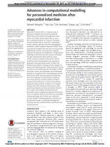
Figure 1. The effect of the sampling frequency f S = 1 kHz on dispersion of 100 values of the resonant frequency f0 computed according to OMI, YM, YMC, A, and Y methods as a function of the length of free decaying signals (i.e. the number of oscillations Losc .) (a) Losc = 5, 10, 15, (b) Losc = 20, 25, 30, (c) Losc = 40, 50, 60, 70, (d) Losc = 80, 90, and 100. Computed values of the
f0 , displayed on vertical plots, correspond to a set of 100 different free
decaying noisy oscillations (S/N = 32 dB) characterized by the same value of the δ = 0.0005 and the resonant frequency f0 = 1.12345 Hz.
4
6th EEIGM International Conference on Advanced Materials Research IOP Conf. Series: Materials Science and Engineering 31 (2012) 012019
IOP Publishing doi:10.1088/1757-899X/31/1/012019
0
f
0 -0.01
f
-0.02
OMI YMC
0
max ( γ ), min ( γ ) [%]
(a)
-0.03
Y
5
15 L osc
10
max ( γ ), min ( γ ) [%]
(b) -3
x 10 0
f
1 0.5
-0.5
0
f
0
-1 20
30
40
50
60
70
80
90
100 L osc
x 10
OMI YM A
0
10
f
5
f
0 0
max ( γ ), min ( γ ) [%]
(c) -3
-5 5
15 L osc
10
0
1
x 10
0.5 0
0
f
f
max( γ ), min( γ ) [%]
(d) -3
-0.5 -1 20
30
40
50
60
70
Figure 2. The effect of the sampling frequency f S = 1 kHz on the minimal
80
γf
0 min
relative errors obtained for computations of the resonant frequency f0 shown in Fig. 1. (a) , (c) Losc = 5, 10, 15; (b), (d) Losc = 20, 25, 30, 40, 50, 60, 70, 80, 90, and 100.
5
90
100L
and the maximal
osc
γf
0
max
6th EEIGM International Conference on Advanced Materials Research IOP Conf. Series: Materials Science and Engineering 31 (2012) 012019
IOP Publishing doi:10.1088/1757-899X/31/1/012019
(a) 1.1236
8.90
4.45
13.35
t [s] OMI YM YM
C
A Y
1.1234 0
f [Hz]
1.1235
1.1233 1.1232 5
10
L
15
osc
(b) 1.123460
17.80
22.25
20
25
26.70 t [s]
f [Hz]
1.123455
0
1.123450 1.123445 1.123440 30
Losc
(c) 35.60
53.41
44.50
1.123455
62.31 t [s]
0
f [Hz]
1.123450 1.123445 1.123440 40
45
50
55
60
65
70 L
osc
(d) 71.21
80.11
1.123450
0
f [Hz]
1.123455
89.01 t [s]
1.123445 80
85
90
95
100 L
osc
Figure 3. The effect of the sampling frequency f S = 6 kHz on dispersion of 100 values of the resonant frequency f0 computed according to OMI, YM, YMC, A, and Y methods as a function of the length of free decaying signals (i.e. the number of oscillations Losc .) Losc = 80, 90, and 100.
(a) Losc = 5, 10, 15, (b) Losc = 20, 25, 30, (c) Losc = 40, 50, 60, 70, (d)
Computed values of the f0 , displayed on vertical plots, correspond to a set of 100 different free decaying noisy oscillations (S/N = 32 dB) characterized by the same value of the δ = 0.0005 and the resonant frequency f0 = 1.12345 Hz.
6
6th EEIGM International Conference on Advanced Materials Research IOP Conf. Series: Materials Science and Engineering 31 (2012) 012019
IOP Publishing doi:10.1088/1757-899X/31/1/012019
max( γ ), min( γ ) [%]
(a) -3
0
f
x 10 0 -5
OMI YMC
0
f
-10 -15
Y
-20 5
15 L
10
osc
0
x 10 5
0 0
f
f
max( γ ), min( γ ) [%]
(b) -4
-5 20
30
40
50
60
70
80
90
100 L osc
max( γ ), min( γ ) [%]
(c) -3
0
f
x 10
OMI YM A
6 4
0
f
2 0 5
15 L
10
osc
0
f
x 10 2
0
0 f
max( γ ), min(γ ) [%]
(d) -4
-2 -4 20
30
40
50
60
70
80
Figure 4. The effect of the sampling frequency f S = 6 kHz on the minimal
γf
90
0 min
and the maximal
relative errors obtained for computations of the resonant frequency f0 shown in Fig. 3. (a) , (c) Losc = 5, 10, 15; (b), (d) Losc = 20, 25, 30, 40, 50, 60, 70, 80, 90, and 100.
7
100 L osc
γf
0
max
6th EEIGM International Conference on Advanced Materials Research IOP Conf. Series: Materials Science and Engineering 31 (2012) 012019
IOP Publishing doi:10.1088/1757-899X/31/1/012019
4. Conclusions The results are primarily reported here to highlight new methods to compute the resonant frequency, f 0 , and the logarithmic decrement, δ , in resonant high-resolution mechanical spectroscopy, HRMS. The performance of different methods and algorithms to compute the resonant frequency for low damping level (e.g. δ = 5×10⁻⁴ ) is listed in the following order: (1) the OMI, (2) the YoshidaMagalas YM, (3) the Yoshida-Magalas YMC, (4) the Agrež A, and finally (5) the Yoshida Y. The Yoshida-Magalas YM method [1, 2] outperforms other IpDFT methods. The YM method yields the smallest dispersion in experimental points of the resonant frequency for different lengths of free decaying oscillations and different sampling frequencies. The effect of the sampling frequency on precision in the computations of the resonant frequency and the logarithmic decrement has received scant attention to date [8] and deserves more. The parametric OMI method is considered as the ‘gold standard’ in low-frequency high-resolution mechanical spectroscopy, HRMS. The point we should like to emphasize is that the sampling frequency is a key factor to reduce dispersion of experimental points computed according to the OMI and IpDFT methods. It is demonstrated that the sampling frequency f S = 6 kHz readily yields better results as compared to usually used f S = 1 kHz in low-frequency mechanical spectrometers operating around the resonant frequency f 0 ≈ 1 Hz. To conclude, the OMI method (Optimization in Multiple Intervals) and the Yoshida-Magalas YM method are recommended to compute the resonant frequency from the exponentially damped timeinvariant harmonic oscillations embedded in an experimental noise. It is not difficult to show, by means of the experimental results reported in [1, 2] and the results described in this volume that the OMI and the YM methods pave the way toward high-resolution mechanical spectroscopy, HRMS. Acknowledgements. This work was supported by Polish National Science Centre under grant No N N507 249040 and No N N507 446639.
References
[1] [2] [3] [4] [5] [6] [7] [8] [9] [10] [11] [12] [13] [14] [15]
Magalas L B and Majewski M 2011 Sol. St. Phen. 184 467-472 Magalas L B and Majewski M 2011 Sol. St. Phen. 184 473-478 Nowick A S and Berry B S 1972 Anelastic Relaxation in Crystalline Solids, Academic Press, New York and London Magalas L B 2003 Sol. St. Phen. 89 1-22 Etienne S, Elkoun S, David L and Magalas L B 2003 Sol. St. Phen. 89 31-66 Magalas L B and Malinowski T 2003 Sol. St. Phen. 89 247-260 Magalas L B and Malinowski T 2003 Sol. St. Phen. 89 349-354 Magalas L B 2006 Sol. St. Phen. 115 7-14 Magalas L B and Stanisławczyk A 2006 Key Eng. Materials 319 231-240 Magalas L B and Majewski M 2008 Sol. St. Phen. 137 15-20 Magalas L B and Majewski M 2009 Mater. Sci. Eng. A 521-522 384-388 Majewski M 2011 Phd Thesis, AGH University of Science and Technology, Kraków, Poland Yoshida I, Sugai T, Tani S, Motegi M, Minamida K and Hayakawa H 1981 J. Phys. E: Sci. Instrum. 14 1201-1206 Agrež D 2009 IEEE Instrumentation and Measurement Technology Conference 1-3 1295-1300 Duda K, Magalas L B, Majewski M and Zieliński T P 2011 IEEE Transactions on 8
6th EEIGM International Conference on Advanced Materials Research IOP Conf. Series: Materials Science and Engineering 31 (2012) 012019
[16] [17] [18] [19] [20] [21] [22] [23] [24] [25] [26]
IOP Publishing doi:10.1088/1757-899X/31/1/012019
Instrumentation and Measurement 60 3608-3618 Magalas L B 2000 J. Alloy Compd. 310 269-275 Magalas L B 1996 J. de Phys. IV 6 (C8) 163-172 Magalas L B and Piłat A 2006 Sol. St. Phen. 115 285-292 Poularikas A D ed. 1996 The Transforms and Applications, CRC Press Inc. Brigham E O 1988 The Fast Fourier Transform FFT and its Applications, Prentice Hall Signal Processing Series Ramirez R W 1985 The FFT Fundamentals and Concepts, Prentice-Hall International Inc. Oppenheim A V, Schafer R W and Buck J R 1999 Discrete–Time Signal Processing, Prentice–Hall Young Randy K 1993 Wavelet Theory and its Applications, Kluwer Academic Publishers Chan Y T 1995 Wavelet Basics, Kluwer Academic Publishers Newland D E 1993 Random Vibrations, Spectral and Wavelet Analysis, Longman Scientific & Technical Qian S and Chen D 1996 Joint Time-Frequency Analysis, The MathWorks, Inc.
9