Nov 8, 1996 - Results of subjective tests show that expert listeners typically ... Since many factors such as frequency,
AES 101 st Convention 1996 November 8-11, Los Angeles
Measuring the Characteristics of “Expert” Listeners Seymour Shlien and Gilbert Soulodre Communications Research Centre 3701 Carling Ave. Ottawa, Ontario, K2H 8S2 Canada
[email protected] [email protected] Abstract Subjective listening tests of digital audio codecs rely on a panel of expert listeners. Experience has shown that members of the listening panel vary in their sensitivities to the various types of coding artifacts. The paper describes the development of psychoacoustic techniques designed to characterize these listeners in order to predict their sensitivities to audio reproduction defects. Results of subjective tests show that expert listeners typically have enhanced sensitivity to one or more particular classes of coding artifact. 0. Introduction The new perception based digital audio codecs, which will become readily available in the next few years, rely on psychoacoustic models of the listener in order to compress and encode the audio signal. These new codecs introduce unique types of distortions and artifacts quite unlike those found in traditional PCM codecs. While most of these distortions and artifacts are likely to be undetectable to the “average” listener, some listeners with superior sensitivities may find them to be clearly audible. In addition, little is known about how individuals vary in their sensitivities and therefore, to meet the expectations of the people who will invest in this new technology, it is necessary to improve our understanding of auditory models of the human listener. Lossy compression techniques used in perceptual coders such as MUSICAM or Dolby’s AC-3 operate on the principle of modifying a signal by reducing the number of bits needed to encode it. This modification is equivalent to adding quantization noise to the signal. However, unlike traditional PCM coding, this quantization noise can manifest itself in many ways, depending on the bit rate, the signal and the coder. The coder may alter the sound of the signal directly by introducing timbral changes to the instruments, rolling off the high frequency content of the signal, or smearing the attacks of some musical instruments (referred to as pre-echo). Alternatively, the coder may add extraneous noises such as beeps, pops, squeaks and static to the signal. Using a psychoacoustic model, the codec attempts to reduce the audibility of these coding artifacts, as far as possible, by placing them at times and frequencies where they are masked by the signal and are thus least noticeable. Though progress has been made in developing psychoacoustic models of the listener, one must still ultimately rely upon real listeners to evaluate and rate the quality of a codec. -1-
AES 101 st Convention 1996 November 8-11, Los Angeles
However, a formal subjective assessment of audio codecs is a lengthy and tedious process. It is not unusual for an expert listener to spend an entire day evaluating a half dozen codecs on a handful of critical audio materials. Furthermore, since there is considerable variation among listeners, the process usually requires a panel of 20 or more expert listeners [1]. The task is further complicated by the fact that codecs have improved dramatically over the past few years and so, for some audio materials, the difference between the original and the compressed signal may be extremely subtle and therefore difficult to detect. Psychoacoustic models are based on the average listener and thus may not represent the gifted listener who is most likely to detect and report audio artifacts. Furthermore, the characteristics of these gifted listeners are quite variable, so that one listener may be unusually sensitive to one class of distortion yet be less responsive to a different class. For example, one listener might be particularly sensitive to “pre-echo” noise preceding a large transient while another listener may be more sensitive to small variations in pitch. This may explain the large variance in subjects’ responses obtained in listening tests, as well as the difficulty of designing a perceptual model [2] which will accurately predict these responses. While there have been many studies on characterizing the hearing-impaired listener, less is known about the gifted listener in the context of coders. By measuring the characteristics of the expert listeners that form a listening panel, we hope to better understand the variations in the ratings obtained in formal listening tests. Furthermore, measuring the characteristics of expert listeners may help in standardizing and calibrating these listening tests, despite possible differences in the balance of listeners on the panel. The measurements can also be used to develop a psychoacoustic model for a particular listener, which could then be used to predict his rating of a particular audio material [2]. Since many factors such as frequency, bandwidth, loudness, duration and timbre simultaneously affect the human perception of an audio signal, psychoacoustic models tend to be complex. Furthermore, direct measurement of the human response to these factors is difficult, since it is hard for people to quantify their response to a particular signal near threshold in a repeatable and consistent fashion. It is not unusual for a series of psychoacoustic measurements to extend over many days for a single listener in order to obtain a comprehensive characterization of that listener’s auditory system [3]. As such, a rigorous approach is not practical for a large population and thus one of the goals of the present study was to investigate alternative measurement techniques. Though these simplified tests may lack some precision in terms of establishing absolute thresholds, the intent is that this would be offset by the ease of administering the tests. Sensitive psychoacoustic tests have traditionally required specialized equipment and facilities not readily available or affordable to some researchers. In the past few years, however, the availability of standard multimedia personal computers has made it much easier to develop and administer psychoacoustic tests. Current audio boards can produce audio signals of the same quality as a CD player, while most computers can now generate
-2-
AES 101 st Convention 1996 November 8-11, Los Angeles
and play an audio signal in real time with enough processing power left over to operate a graphical user interface. For many psychoacoustic tests, the only additional requirements are an A/D converter and a pair of good quality headphones. 1. Overview The paper has several goals. First, it is of interest to examine how thresholds for “expert listeners” differ from those of the general population of listeners, as well as how they vary among themselves. Second, new methodologies are introduced for measuring these characteristics in a rapid and efficient manner. The various audio coding artifacts are also classified into groups. As a final goal, the listener’s sensitivities to these groups of artifacts are measured to determine if a correlation exists between a listener’s thresholds and his ability to discriminate small coding artifacts. Section 2 of the paper describes the new simplified measurement methodologies. Three tests are described which are designed to measure the listener’s: 1) absolute threshold of hearing, 2) sensitivity to pitch variations, and 3) sensitivity to short temporal events. Typical and non-typical results are shown for the general and expert listeners. Section 3 of the paper describes an attempt to classify some of the coding artifacts introduced by lossy compression techniques as well as efforts to measure the listener’s sensitivities to these artifacts. 2. Psychoacoustic Measurements 2.1 Introduction The human auditory system is logarithmically responsive to both the frequency and the amplitude of an auditory signal. Typically it is modeled in several stages. Those frequencies of the signal which fall in the range from 1 to 3 kHz are amplified by the mechanical characteristics and geometry of the middle ear. The signal is then transferred to the cochlea where the individual hair cells in the basilar membrane each respond to a particular frequency range. Effectively, the basilar membrane maps the linear frequency scale to a nonlinear pitch or mel scale. Furthermore, since the filter responses of the hair cells are spread out in both frequency and time, the signal is effectively smeared thus introducing various masking effects which reduce the listener’s ability to resolve small temporal and frequency differences. Psychoacoustic models attempt to explain these effects using mathematical models derived through experimental measurements. Many of the differences between various audio codecs are attributable to the differences in their psychoacoustic models. The tests conducted in the present study concentrated on measuring the innate perceptual limitations of the subject and avoided, as much as possible, measurement of any cognitive component. To illustrate this point, consider that the ability to detect small differences in pitch is an innate ability, whereas the ability to determine which of two tones is higher in
-3-
AES 101 st Convention 1996 November 8-11, Los Angeles
pitch, when the difference is small, depends to some extent on the subject’s musical training and ability. The subject’s performance improves while acquiring a new skill but later declines when fatigue and boredom set in. These cognitive factors introduce more variability into the results and reduce the repeatability of the test. Many thresholds depend on one or more variables. Conventional psychoacoustic measurement techniques would attempt to estimate the threshold on a point-by-point basis in the parameter space. By assuming a parametric model a priori, it is not necessary to estimate the threshold at each point very accurately. The parametric curve that provides the best fit among all the sample measurements reduces the measurement uncertainty. The test to determine the absolute hearing threshold relied on the cooperation and honesty of the listeners to adjust the loudness of a tone to their threshold of perception. Though this methodology introduces a small zone of uncertainty where the listener cannot decide whether the tone is truly audible or imagined, more precise measurements were not required for this study. Other tests did not rely on the listener’s judgment but instead used a forced choice approach wherein the subject was forced to choose among two or more stimuli regardless of whether any differences could be heard. In such a test there is always a significant probability that the subject might, by chance, correctly discriminate between two stimuli when, in fact, no difference is detected. As such, this methodology requires many more trials in order to better establish the subject’s true threshold. The use of adaptive measurement techniques [4] was considered since they often require fewer trials in order to determine a threshold. However, these methods can become quite tedious during final convergence and so, for the experiments described in this section, samples were chosen at random from a parameter space so that listeners encountered easy trials interspersed with the more difficult ones. In many of the tests, the listener was not given any time limit and could replay the trial as many times as desired. In retrospect, however, it would be preferable to place certain time limits in order to shorten the duration of the test. 2.2 Test of Absolute Threshold of Hearing Above 4kHz Perceptually based audio codecs often assume that the listener's hearing declines in the higher frequencies. When there are insufficient bits to encode the signal, the coder may assign fewer bits to the information in the high frequencies. Listeners with better than normal hearing in the high frequencies may detect high frequency attenuation or extraneous artifacts (such as chirps, beeps and squeaks) in the high frequency band. These effects become more annoying when they are signal dependent and fade in and out unpredictably. The test of absolute threshold of hearing (as well as the other tests) was implemented on a SPARC-10 computer using Beyer DT-901 headphones. The signal levels in the headphones were calibrated using a General Radio 1565-B sound level meter fitted with a 9A Type earphone coupler. Given that the focus of the study was to examine the
-4-
AES 101 st Convention 1996 November 8-11, Los Angeles
audibility of artifacts created by low bit rate coders, the test was customized to measure the listener’s threshold in the frequency range from 4 to 24 kHz. Using the computer’s mouse, the subject graphically adjusted the loudness of a pulsating tone in ±1dB increments until converging upon his hearing threshold. The process was repeated for each of as many as 40 tones spaced 0.5 kHz apart. An example of the results from this test (Subject TT) are shown in Figure 1. The figure also represents the graphical interface employed by the subjects during the test. In the figure, each of the vertical bars represents the frequency of a test tone, while the height of the bar indicates the level at which the listener could first detect the presence of the tone. Figure 2 shows the absolute thresholds of hearing above 6 kHz for five of the subjects tested. The bold curve represents the analytical expression derived by [5] to depict an average listener. The results clearly indicate that large variations exist among individuals. It can be seen that among the results shown in Figure 2 are listeners who demonstrate both significantly greater and poorer high frequency acuity. Therefore, while a psychoacoustic model based on this average curve might provide sufficient performance for Subjects UH, ML and DB, such a model would perform inadequately for Subjects RP and JD. That is, Subjects RP and JD are likely to detect variations in the high frequency content of a coded signal based on such a psychoacoustic model. Generally speaking, roughly half of the subjects tested demonstrated better high frequency acuity than predicted by the analytical expression for an average listener. These results will be discussed further in Section 2.5 below. 2.3 Pitch Discrimination In the work to classify the various types of artifacts created by perception based lossy codecs, it was found that errors in the pitch of the coded signal often occur. This error typically manifests itself as either a modulation of the pitch of a note around some average value, or the inability of the codec to adequately track the transition from one note to the next. The ability to detect small changes in pitch is an important asset for any serious string player and therefore it was felt that some listeners might be more sensitive to the errors in pitch created by some codecs. As such, the tests described in this section were conducted to measure the listener’s sensitivity to small variations in frequency. The Just Noticeable Variation in Frequency (JNVF), the critical bandwidth and the frequency to distance mapping along the unwound cochlea are all believed to be related [6]. Most perceptual models of the ear involve a transform of the signal from the frequency scale to an internal pitch representation based on the mel, Bark or critical bandwidth scale. Though the literature leaves the impression that there is a fixed mapping between frequency and the critical band scale, the results of the present study imply that there are many individual variations to this relationship.
-5-
AES 101 st Convention 1996 November 8-11, Los Angeles
The frequency modulation threshold test described in [6] formed the basis of the test described in this section. The test involved playing a tone whose frequency varied from f∆f to f+∆f at a modulation rate of four times per second. This modulation rate was selected since it is the rate at which listeners are most sensitive to changes in frequency [6]. If ∆f is large enough, the listener hears a wavering pitch, otherwise the tone sounds steady (i.e. unmodulated). The threshold, ∆fT, where the listener is able to detect a wavering pitch typically increases with frequency. The experimental procedure consisted of playing a sequence of tones with random frequency, f, and frequency modulation, ∆f. The process was repeated with 100 to 200 stimuli, whose parameters were logarithmically distributed over the frequency range of interest. For each stimulus, the listener indicated via the computer interface whether the tone sounded steady or wavering. Whenever there was any uncertainty, the listener was instructed to indicate that the signal sounded unmodulated. Figure 3 shows the results from this test for Subject TT. In the figure, the horizontal axis indicates the frequency, f, of the tone, while the vertical axis indicates the amount by which the tone is modulated (i.e. ∆f). The asterisks (*’s) indicate the stimuli which the listener identified as sounding modulated, while the open circles (o’s) indicate those samples which sounded steady. The curve separating the two regions was determined by a procedure described in the Appendix. The results shown in this figure indicate that there is a well defined threshold where the sound of the signal changes for a particular listener. Stray errors sometimes occurred when the listener accidentally selected the wrong button on the mouse. Furthermore, some inconsistencies around threshold are obviously due to variations in the listener’s criterion for detecting the modulated signal. Figure 4 shows a composite of the results of the pitch sensitivity test for five of the listeners tested. The bold line represents an analytical piece-wise linear approximation to an average listener as proposed in [6]. The figure demonstrates that significant individual differences exist among the listeners tested. Furthermore, some listeners demonstrate large differences from the approximation of an average listener. For example, the results demonstrate that Listener DB is significantly more sensitive to variations in pitch than would be predicted by the analytical expression. The Just Noticeable Variation in Frequency is believed to map to a constant step size along the basilar membrane. Furthermore, the JNVF has also been shown to be related to the critical bandwidth by a constant factor of about 25. Figure 5 shows the relationship of the critical band rate (mels) and frequency as proposed by Zwicker and Fastl [6]. Also shown in the figure is the frequency to mel mapping that would be obtained using Subject DB’s results. Clearly, a psychoacoustic model employing a mapping based on Subject DB’s pitch sensitivity would require a much larger range along the mel scale.
-6-
AES 101 st Convention 1996 November 8-11, Los Angeles
2.4 Temporal Sensitivity Perception based codecs rely on time-frequency representation schemes in order to encode the audio signal and are thus susceptible to "pre-echo" and “post-echo” effects. Frequency representations of a signal require a large number of bits in order to completely encode large transients. When the number of bits available is insufficient, the resulting quantization error introduces an audible noise in the neighborhood of the sudden attack, that is, the quantization error introduces artifacts before and after the signal transient. An artifact occurring prior to the signal transient is referred to as a pre-echo, while one occurring after the transient is called a post-echo. Figure 6 illustrates some severe pre-echo noise produced by a perception based codec. The upper curve in the figure represents the time domain waveform of the unprocessed signal (castanets). It can be seen that the attack of a transient begins at about sample 18260. The signal is relatively silent just prior to this transient. In the lower curve, which represents the processed signal, it can be seen that the previously silent period (samples 18200 to 18260) now contains pre-echo noise. Pre-echoes are generally more audible just before a transient where the ambient signal is low. The duration and intensity of the pre-echo or post-echo depends on the spectral resolution of the compression technique as well as the bit rate (and hence the number of bits available). Due to pre- and post-masking effects these artifacts are inaudible to most listeners, although some listeners appear to be very sensitive to these effects. The following test was conducted in order to quantify and confirm these sensitivities. Temporal sensitivity was measured by determining the threshold for detection of a quiet gap in an ongoing sound [7]. Two identical noise bursts each lasting 0.15 seconds were played to the listener. In one of the bursts there was a short quiet gap where a small interval of the noise was attenuated by a factor varying between 0 and -40 dB. The duration of the gap was also varied (from 0.0 to 7.0 milliseconds). The listener was asked to decide which of the noise bursts had the short gap. In this way the listener’s threshold for detecting these gaps was determined as a function of duration and level. Figure 7 shows the results of this temporal sensitivity test for Subject TT. The horizontal axis represents the duration of the gap in milliseconds, while the vertical axis indicates the depth of the gap in decibels. The asterisks (*’s) indicate the instances where the listener was able to correctly identify the stimulus containing the gap, whereas the open circles (o’s) indicate the instances where the listener was unable to detect the gap. When the length of the gap is less than a certain threshold (depending upon the attenuation factor), the two noise bursts become indistinguishable and the listener is correct only about 50 percent of the time. The line segment separating the two regions was determined by a procedure described in the Appendix. The results shown in this figure indicate that there is a sharply defined threshold where the sound of the signal changes for a particular listener. As suggested by this line, gaps of shorter duration require more attenuation in order to be audible.
-7-
AES 101 st Convention 1996 November 8-11, Los Angeles
The results of the temporal sensitivity test are shown in Figure 8 for five of the subjects tested. The measurements indicate that there are considerable variations among the listeners’ temporal sensitivities. Some listeners, such as Subject ML and Subject DB, are exceptionally sensitive to temporal changes in the signal and can detect artifacts with durations of less than a millisecond. It should be noted that for this test in particular, the subject’s sensitivity may improve with experience as he learns to detect more subtle artifacts. Nevertheless, the amount of improvement was found to be much smaller than the differences among the individuals. 2.5 Discussion of Results of Psychoacoustic Measurements Some reduction of the data is necessary in order to facilitate comparisons across subjects and tests. For the absolute threshold of hearing test, listeners were ranked on the basis of their 40dB high frequency cutoff. These results are listed in Table 1 in descending order of subject performance. Comparing Figure 2 with Table 1 indicates that this quantification procedure appears reasonable. For example, Subjects JD and RP who are ranked in the table as most sensitive to high frequency signals are well above the average curve in the figure, while Subjects ML and UH who ranked among the least sensitive, were significantly below the average curve.
Subject JD RP SK FG HT TT RR average DB BB ML RV UH
40 dB cutoff in kHz 17.0 kHz 17.0 15.5 15.0 14.5 14.5 14.0 14.0 13.5 13.5 12.5 12.5 9.0
Table 1. Absolute threshold of hearing (40 dB cutoff frequency) listed in descending order. The value for an average listener was taken from [5]. To simplify the results of the frequency modulation test, the subjects were ranked on the basis of their frequency resolution at 1kHz (see Table 2). This appears to be a reasonable indicator since the curves in Figure 4 have the same general shape and do not overlap below 2kHz.
-8-
AES 101 st Convention 1996 November 8-11, Los Angeles
Finally, for the gap sensitivity test (Figure 8), subjects are ranked in Table 3 by the percentage of stimuli that were correctly identified as having the gap. Subject DB UH RR FG ML RW DM BT average JT JD AK GG RP SK TT
Frequency Resolution at 1 kHz 1.7 Hz 3.0 3.0 3.0 4.0 4.0 6.0 6.0 6.5 7.0 7.0 8.0 10.0 11.0 15.0 19.0
Table 2. Frequency modulation sensitivity at 1kHz in descending order. The value for an average listener was taken from [6]. Subject ML DB HT FG JD SK TT RR UH AK RP
Temporal Sensitivity Score 88 % 85 84 82 81 78 78 76 75 74 73
Table 3. Gap sensitivity in descending order. Scores indicate the percent of stimuli correctly identified as having the gap. In looking at the results of these tests, it is interesting to observe that the ranks of most of the subjects were not consistent in the three tasks. For example, UH was well below average in the absolute threshold of hearing test, but ranked second in the frequency modulation test. Similarly, Subject ML demonstrated a significant hearing loss in the higher frequencies, yet ranked first in the temporal sensitivity test. On the other hand, Subject RP ranked first in the -9-
AES 101 st Convention 1996 November 8-11, Los Angeles
absolute threshold test, but was at the low end of the scale for the other two tests. Also, Subject DB, whose ability to detect variations in pitch far exceeded the average, demonstrated only average performance in the absolute threshold test. The results of this section, despite the limited sample size, suggest several conclusions. First, it appears that hearing aptitude can manifest itself in a variety of ways along many dimensions and therefore, the traditional absolute threshold of hearing test is quite inadequate as an indicator of hearing acuity or listener expertise. Moreover, there is significant variance among listeners in their ability to resolve these dimensions. Secondly, a listener may demonstrate expertise (hearing acuity) in one or more areas without being an expert in all areas. Furthermore, listeners can have significant deficiencies in some aspects of their hearing while demonstrating very high levels of expertise in other areas. Interestingly, of the listeners measured in the present study, none demonstrated an extremely high level of expertise in all of the areas tested. Therefore, the results tend to dismiss the concept of a “golden ear” listener who can detect all classes of artifacts. From the point of view of developing a psychoacoustic model for a perceptual coder, the results suggest that, due to the large variations among listeners, a model based on an average listener is probably inadequate. Finally, the findings indicate that the ability of an individual to act as an expert listener in a subjective test depends on the type of artifacts to be detected in that test. 3. Detection of Audio Coding Artifacts 3.1 Compilation and Classification of Audio Materials The tests described in Section 2 used artificially generated stimuli in order to measure a listener’s absolute threshold, as well as pitch and temporal sensitivities. In this section, tests are described which were conducted using materials processed by a variety of perceptual coders. The intent of these tests is to determine whether the variations in the listeners’ expertise found in the previous section would also occur when auditioning these coded materials. A library of audio materials containing a variety of coding artifacts was gathered from formal listening tests conducted in our laboratory over the past several years. Each of these materials was then analyzed separately by three “expert” † listeners who identified all of the audible artifacts in each audio material. Following that, the three listeners worked together to categorize the artifacts into different classes. Among these classes were artifacts encompassing temporal, pitch, timbral, spatial and masking effects. In order to obtain a comprehensive collection of artifacts, materials processed through both subband based and transform based coders where used. The entire process, which took several weeks to complete, was conducted using a computer based playback system in a critical listening environment. †
The listeners were known from past formal subjective experiments to have a high level of expertise.
-10-
AES 101 st Convention 1996 November 8-11, Los Angeles
A set of short (1 s duration) audio excerpts were then chosen from the library for use in the tests. These excerpts were carefully chosen such that they contained only one type of coding artifact. For example, excerpts containing both pre-echo and high frequency rolloff were not used. Also, the excerpts were selected so as to provide a range in the severity of the different artifacts. A total of 19 excerpts were selected containing artifacts related to pre-echo, unmasking of quantization noise (graininess), and high frequency effects. The excerpts were then used in a series of subjective experiments to determine listeners’ sensitivities to these three types of artifacts. The unprocessed original versions of the 19 excerpts were also collected for the tests. 3.2 Determining Thresholds Using Non-adaptive Methods In this section, tests are described which were designed to determine a listener’s threshold of detection using non-adaptive methods. Specifically, the tests consisted of playing four randomly ordered stimuli to the listener over headphones. Three of the stimuli, which were identical, consisted of the original unprocessed signal, and thus did not contain any coding artifacts. The fourth stimulus was the processed (coded) excerpt containing a given artifact. The listener’s task was to identify the processed excerpt from among the four stimuli. The process was repeated five times in order to reduce the statistical probability of a listener correctly identifying the processed excerpt purely by guessing. Based on the binomial distribution, the expected distribution for a listener who was guessing is given by (0, 0.237), (1, 0.3955), (2, 0.2637), (3, 0.0879), (4, 0.0146) and (5, 0.0010) [8]. In each of the parentheses, the first number represents the number of times (out of 5) that a listener correctly identified the processed excerpt, while the second number indicates the probability of this occurring by chance. For example, the probability of a listener guessing correctly five times is 0.0010. Prior to each test, the subject went through a familiarization process in which he could directly compare the processed and unprocessed excerpts. The process of comparing the original to the compressed excerpt involves both perceptual and cognitive tasks. Although the audio excerpts were quite short, there was still a great amount of information for the listener to process, and it was necessary for the listener to focus his attention on various parts of the signal in order to identify the differences. When the difference was subtle (i.e. when the coding artifact was not severe), the cognitive aspects of the task may have dominated. The results of the test could then vary with time depending upon the current state of the subject (i.e. learning and fatigue effects). Three separate tests were conducted for each subject. Seven subjects took part in these tests, many of whom were included in the tests of Section 2. In the first test, the coded excerpts contained varying degrees of pre-echo artifacts. The excerpts consisted of recordings of castanets and a glockenspiel. An example of the pre-echo artifact for the castanets was seen in Figure 6. These materials tend to be most susceptible to pre-echo artifacts because of the sharp transients that they contain.
-11-
AES 101 st Convention 1996 November 8-11, Los Angeles
In the second test, the listeners were asked to identify coded excerpts having varying degrees of graininess. Graininess refers to a roughness or granularity that can result when materials are processed through a perceptual coder. Graininess is often associated with quantization noise that is not fully masked by the signal and is in the same frequency range as the signal. A recording of a bass clarinet holding one note was used for this test. The bass clarinet was found to be good at revealing graininess, because of its rich harmonic structure. Figure 9 shows a spectrogram of the unprocessed bass clarinet. The horizontal axis represents time in seconds, while the vertical axis shows frequency. Darker areas on the spectrogram indicate where the signal level is stronger, whereas the lighter areas indicate lower levels. Figure 10 shows the corresponding spectrogram of the bass clarinet processed through a perceptual coder. The graininess in the coded excerpt (Figure 10) can be seen as white patches randomly distributed throughout the spectrogram. These patches indicate “holes” in the signal at different frequencies, where for short instances of time, that portion of the signal was missing. The third test was designed to assess each listener’s ability to detect changes in the high frequency spectrum of the signal. These changes consisted of either an attenuation or boost of some of the higher frequencies of the signal. A recording of a female vocalist (acapella) was used in this test. Figure 11 provides a spectrogram of the unprocessed excerpt of the female vocalist. It can be seen that a significant amount of signal is present up to 20kHz. In Figure 12, however, which shows the spectrogram of a coded version of the excerpt, it can be seen that significant portions of the signal are missing in the higher frequencies. The results of the pre-echo test are given in Figure 13. Two separate analysis of the data are presented in this figure. The horizontal axis indicates the seven codecs used in this test which have been arbitrarily labeled (PA, PB, PC, etc.). The dashed line in the figure is related to the vertical axis on the left-hand side of the graph, and represents the number of subjects who could detect the artifact from a given codec. For example, all seven listeners could detect the pre-echo created by codec PA, whereas none of the listeners could detect the artifact created by codec PG. To decide whether or not a listener could reliably detect a given artifact a 98.5% confidence level was used. This corresponds to a listener being able to correctly identify the excerpt containing the artifact in at least 4 out of 5 trials. The labels on the right-hand vertical axis represent the seven subjects who participated in the tests. The x’s and o’s in the figure are related to these labels, and indicate whether or not a listener could detect an artifact from a particular codec. The x’s indicate that the artifact was detected, whereas the o’s indicate that it was not detected. For example, the top row of x’s and o’s correspond to Subject UH’s results. The first x on the left indicates that Subject UH detected the artifact in codec PA, whereas the next two o’s indicate that UH could not detect an artifact in codecs PB and PC. Also, it should be noted that listeners have been ordered with the best performer at the bottom of the graph and the poorest performer at the top. Interestingly, the dashed line forms a rough boundary between the excerpts where the artifacts could be detected and those excerpts where the artifacts were not detected.
-12-
AES 101 st Convention 1996 November 8-11, Los Angeles
The results of Figure 13 suggest that there is agreement among the listeners as to which codecs produced the more audible artifact. For example, all subjects could detect the artifact produced by codec PA, whereas none of the listeners could detect an artifact from codec PG. Therefore, it is reasonable to talk about the severity of an artifact along a continuous scale. Figure 14 show the results of the test to assess the listener’s sensitivity to graininess. In this test, excerpts from six different codecs were used. Again, it can be seen that there is good agreement among the listeners regarding the severity of the artifacts. The results of the measurements of the listeners’ sensitivity to changes in the high frequencies are given in Figure 15. Here, the agreement among listeners, while still good, is not as good as for the previous two tests. This may be due, in part, to the fact that both high frequency boosts and attenuations were present in the coded excerpts. Subject RR SK FG RP TT UH ML
High Freq Response 5 of 6 5 5 3 2 1 1
Graininess 5 of 6 0 5 6 6 1 4
Pre-echo 4 of 7 2 6 2 3 2 5
Table 4. Number of coded excerpts correctly identified by each listener. It is interesting to compare each subject’s performance across the three tests, as was done in Section 2. This comparison can be summarized as in Table 4 which shows the number or coded excerpts that each listener was able to reliably detect in the three tests. The main result from these tests is that it is possible for a listener to be sensitive to one type of coding artifact while being relatively insensitive to others, that is, there are different ways in which a listener can demonstrate expertise. For example, Subject SK appears to be very sensitive to changes in the high frequency response of the signal, while being relatively insensitive to both graininess and pre-echo. Conversely, Subject ML was much more sensitive to pre-echo than to high frequency effects. The results of these tests, which used excerpts from real codecs, tend to support the findings of Section 2.
-13-
AES 101 st Convention 1996 November 8-11, Los Angeles
4. Summary and Discussion The paper described a series of auditory tests implemented on a Unix workstation for characterizing the detection capabilities of normal and gifted listeners. The tests conducted so far have concentrated on measuring the high frequency hearing thresholds and estimating the temporal and frequency resolutions of the listeners. Considerable variations were found among the test subjects and in many instances, a listener who performed below average in one test showed superior performance in another. The results also tend to dismiss the notion of a “golden ear” listener who is gifted in all areas of auditory perception. Due to the small sample size of test subjects, the results are still preliminary and many other factors remain to be investigated. One of the unresolved issues is whether to make the loudness of the test signal adjustable to suit the individual preferences of the test subject, or whether to have it fixed by the hardware and software. In the present study, the loudness was fixed but some subjects indicated that the signal was too loud for comfort, while others wanted it louder. Allowing the loudness to be variable would introduce another degree of freedom which may confound the results. For example, the slopes of masking curves with frequency are known to flatten when the masker is louder. It would be desirable to expand the series of tests to measure the listener’s sensitivities to other factors. For example, informal tests revealed that some listeners have exceptional sensitivities to small differences in loudness, while others were exceptional in their excellent memory for tonal and rhythmic sequences. The noise masking tone and the tone masking noise curves, which are an essential component of any psychoacoustic model, also varied among listeners. Furthermore, these masking curves depend on both the frequency and loudness of the masker, and we have yet to develop a simple test which would allow quick comparisons among individuals. Though it is desirable to expand the series of tests, carrying out these tests on many subjects is tedious and many of the (unpaid) subjects have limited availability. As such, it would be ideal if the entire sequence of tests could be conducted in less than one hour of the subject’s time. The tests in the present study were conducted in a quiet office environment where computer fan noise and other distractions were present. The output signal from the audio board was analog and not completely free of noise. Presently, the software is being ported to a PC in a Windows 95 environment which will provide more freedom to use better audio equipment and allow the tests to be conducted in an audio chamber. In order to promote further collaborations in the field, the authors plan to make the software for running some of these tests freely available over the network. One of the difficulties in the field of psychoacoustic measurements is that there are many varying factors, many different tests and few standards. With the gradual introduction of digital audio compression techniques, the importance of the field will continue to grow, and it is hoped that renewed interest in the field will lead to better models and measurement techniques.
-14-
AES 101 st Convention 1996 November 8-11, Los Angeles
5. Acknowledgments The authors would like to thank the many subjects who generously donated their time for these tests. This study would not have been possible without their help. Also, the helpful comments by our colleagues at the CRC is gratefully acknowledged. 6. References [1]
ITU-R Recommendation BS.1116, “Methods for the subjective assessment of small impairments in audio systems including multichannel sound systems”.
[2]
W. Treurniet, “Simulation of Individual Listeners with an Auditory Model”, presented at the 100th convention of the AES, preprint 4154, 1996.
[3]
D.M. Johnson, C.S. Watson and J.K. Jensen, “Individual differences in auditory capabilities”, J. Acoust. Soc. Am. 81(2), pp. 427-438, 1987.
[4]
H. Levitt, “Transformed up-down methods in psychoacoustics”, J. Acoust. Soc. Am. 49(2), pp. 467-477, 1970.
[5]
E. Terhardt, G. Stoll, and M. Seewann, “Algorithm for extraction of pitch and pitch salience from complex tonal signals”, J. Acoust. Soc. Am. 71(3), pp. 679-688, 1982.
[6]
E. Zwicker and H. Fastl, Psychoacoustics Facts and Models, Springer-Verlag, Berlin, 1990.
[7]
D.M. Green and T.G. Forrest, “Temporal gaps in noise and sinusoids”, J. Acoust. Soc. Am. 86(3), pp. 961-970, 1989
[8]
L. Sachs, Applied Statistics - A Handbook of Techniques, Springer-Verlag, New York, 1982.
[9]
T. W. Anderson, An Introduction to Multivariate Statistical Analysis, John Wiley and Sons Inc., New York, pp. 133-134.
[10] D. F. Morrison, Applied Linear Statistical Methods, Prentice-Hall Inc., Englewood Cliffs, N.J. USA, pp. 258-259. [11] T. Masters, Practical Neural Network Recipes in C++, Academic Press, Boston, 1993. [12] W.H. Press, B.P. Flannery, S.A. Teukolsky and W.T. Vetterling, Numerical Recipes in C, Cambridge University Press, 1992.
-15-
AES 101 st Convention 1996 November 8-11, Los Angeles
7. Appendix The method for finding the parameters of the threshold curve (e.g. Figures 3 and 7) is quite novel and is described in this Appendix. The parametric form of the equation was selected by trial and error. For the frequency modulation test, the expression used is given by log10 ( ∆f T ) =
10 . A + B log10 ( f )
,
A-1
where frequency, f, and the frequency deviation threshold, ∆f T , are both specified in hertz, and the parameters A and B are to be estimated from the listener’s data. For the gap sensitivity test, a simple linear model was assumed. The problem of finding the curve (or surface) which separates the two classes of data in a parameter space is similar to the problem encountered in statistical pattern recognition. Linear methods such as discriminant analysis [9] [10] were precluded as the sample data was not Gaussian distributed. Instead, it was necessary to develop a new estimation procedure. The parameters of the curve are estimated using a minimization procedure which attempts to reduce the misfit of the curve with the experimental data. Since the curve tries to separate the data space into two regions (i.e. the regions where the listeners hear and do not hear the audio stimulus), the measure of misfit is determined by counting the number of samples which fall on the wrong side of the curve. There are two types of classification errors: (1) where the subject hears a stimulus which he should not hear based on the model and (2) where the subject does not hear the stimulus when he should. For the frequency modulation test, which relied on the listener’s honesty, it was possible to minimize the sum of the two errors. However, for the gap sensitivity test, where there was a 50 percent chance of the listener identifying the correct stimulus even when it was inaudible to the listener, only one type of error was minimized. Gradient optimization procedures require that the misfit measure be a continuous function of the estimated parameters A and B. To ensure continuity, the contributed misclassification error was weighted by the vertical distance of the sample from the curve, x, using the function s( x ) =
10 . 10 . + e − cx
,
A-2
where c is a chosen parameter. This weighting function is identical to the activation function commonly used in artificial neural network models [11]. When the sample falls directly on the curve (i.e. x=0.0), the error contribution is 0.5. For positive or negative values of x, the contribution approaches 1.0 or 0.0 respectively at a rate which is -16-
AES 101 st Convention 1996 November 8-11, Los Angeles
dependent on the value of the constant c. From experience, it was found that c determines the sharpness of the minimum as well as the likelihood of encountering multiple minima. A suitable value for c was chosen by experimentation. When only one minimum is encountered, the gradient search technique, e.g. [12] finds the optimal parameters efficiently. When multiple minima are encountered however, the gradient technique will likely converge to the wrong set of parameters and the curve is clearly inappropriate for the experimental data. (Multiple minima frequently occur when the sample size is inadequate.) When many minima occur, it is preferable to use an exhaustive search procedure. The continuous parameter space is replaced with a rectangular grid of points and the parameters are estimated to the accuracy of the point spacing in the grid. This procedure is quite practical for a two-dimensional search space but would not be recommended for higher dimensional spaces. The number of test samples is an important consideration as it determines both the duration of the test as well as the repeatability of the results. Since the listener is able to process a sample stimulus in a few seconds, the listener is encouraged to provide between 100 and 200 samples.
-17-
AES 101 st Convention 1996 November 8-11, Los Angeles
Figure 1. Absolute threshold of hearing test results for Subject TT.
50
DB
UH
Terhardt et al.
Sound Pressure Level, dB
RP
JD
40 ML 30
20
10
0 6
8
10
12
14
16
18
Frequency, kHz
Figure 2. Absolute thresholds of hearing measured for five subjects. The bold curve represents an "average" listener as given in [5].
-18-
AES 101 st Convention 1996 November 8-11, Los Angeles
Figure 3. Results of modulated pitch sensitivity test for Subject TT. The curve was derived using the method described in the Appendix.
Figure 4. Just noticeable variation in frequency measured for five subjects. The bold curve represents a piecewise linear approximation to an “average” listener [6]. -19-
AES 101 st Convention 1996 November 8-11, Los Angeles
12000 DB
10000
Mels
8000 6000 4000 Zwicker
2000 0
0
5
10 frequency, kHz
15
20
Figure 5. Frequency to mel mapping function as defined by [6]. The upper curve represents how the mapping might look for Subject DB.
Figure 6. Example of pre-echo created by a perception based lossy codec. The upper curve represents the unprocessed signal while the lower curve is the processed signal. Note the pre-echo noise from sample 18200 to sample 18260 in the lower curve. -20-
AES 101 st Convention 1996 November 8-11, Los Angeles
Figure 7. Results of gap sensitivity test for Subject TT. The curve was derived using the method described in the Appendix.
ML
0
JD
DB
RP
UH
-5
Gap Depth, dB
-10 -15 -20 -25 -30 -35 -40 1
2
3
4
5
6
Gap Duration, msec Figure 8. Gap sensitivity curves for five subjects.
-21-
7
AES 101 st Convention 1996 November 8-11, Los Angeles
Figure 9. Spectrogram of unprocessed bass clarinet.
-22-
AES 101 st Convention 1996 November 8-11, Los Angeles
Figure 10. Spectrogram of processed bass clarinet. White patches indicate where portions of the signal are missing, resulting in graininess.
-23-
AES 101 st Convention 1996 November 8-11, Los Angeles
Figure 11. Spectrogram of unprocessed female voice.
-24-
AES 101 st Convention 1996 November 8-11, Los Angeles
Figure 12. Spectrogram of processed female voice. Note that much of the high frequency content of the signal is missing.
-25-
AES 101 st Convention 1996 November 8-11, Los Angeles
Pre-echo x - detected o - not detected
Number of subjects who detected the artifact
7 6
x
o
o
x
o
o
o
UH
5
x
x
o
o
o
o
o
RP
4
x
x
o
o
o
o
o
SK
3
x
x
x
o
o
o
o
TT
2
x
x
x
x
o
o
o
RR
1
x
x
x
x
x
o
o
ML
0
x
x
x
x
x
x
o
FG
PA
PB
PC
PD
PE
PF
PG
Codec
Figure 13. Results of pre-echo test. The horizontal axis indicates the seven codecs used in this test which have been arbitrarily labeled (PA, PB, PC, etc.). The dashed line in the figure is related to the vertical axis on the left-hand side of the graph, and represents the number of subjects who could detect the pre-echo artifact from a given codec. The labels on the right-hand vertical axis represent the seven subjects who participated in the test. The x’s and o’s in the figure are related to these labels, and indicate whether or not a listener could detect the artifact from a particular codec. The x’s indicate that the artifact was detected, whereas the o’s indicate that it was not detected. The listeners have been ordered with the best performer at the bottom of the graph and the poorest performer at the top.
-26-
AES 101 st Convention 1996 November 8-11, Los Angeles
Graininess x - detected o - not detected
Number of subjects who detected the artifact
7 6
o
o
o
o
o
o
SK
5
x
o
o
o
o
o
UH
4
x
x
x
x
o
o
ML
3
x
x
x
o
x
x
FG
2
x
x
x
x
x
o
RR
1
x
x
x
x
x
x
RP
0
x
x
x
x
x
x
TT
GA
GB
GC
GD
GE
GF
Codec
Figure 14. Results of graininess test. The horizontal axis indicates the six codecs used in this test which have been arbitrarily labeled (GA, GB, GC, etc.). The dashed line in the figure is related to the vertical axis on the left-hand side of the graph, and represents the number of subjects who could detect the graininess artifact from a given codec. The labels on the right-hand vertical axis represent the seven subjects who participated in the test. The x’s and o’s in the figure are related to these labels, and indicate whether or not a listener could detect the artifact from a particular codec. The x’s indicate that the artifact was detected, whereas the o’s indicate that it was not detected. The listeners have been ordered with the best performer at the bottom of the graph and the poorest performer at the top.
-27-
AES 101 st Convention 1996 November 8-11, Los Angeles
High Frequency Response x - detected o - not detected
Number of subjects who detected the artifact
7 6
x
o
o
o
o
o
UH
5
x
o
o
o
o
o
ML
4
o
x
x
o
o
o
TT
3
x
x
o
o
o
x
RP
2
x
x
o
x
x
x
FG
1
x
x
x
x
x
o
SK
0
x
x
x
x
x
o
RR
HA
HB
HC
HD
HE
HF
Codec
Figure 15. Results of high frequency response test. The horizontal axis indicates the six codecs used in this test which have been arbitrarily labeled (HA, HB, HC, etc.). The dashed line in the figure is related to the vertical axis on the left-hand side of the graph, and represents the number of subjects who could detect the high frequency artifact from a given codec. The labels on the right-hand vertical axis represent the seven subjects who participated in the test. The x’s and o’s in the figure are related to these labels, and indicate whether or not a listener could detect the artifact from a particular codec. The x’s indicate that the artifact was detected, whereas the o’s indicate that it was not detected. The listeners have been ordered with the best performer at the bottom of the graph and the poorest performer at the top.
-28-