Akaroa2: Exploiting Network Computing by Distributing Stochastic Simulation G. C. Ewing and K. Pawlikowski Department of Computer Science D. McNickle Department of Management University of Canterbury Christchurch, New Zealand
[email protected] Abstract. In this paper we discuss an application of network computing in the area of stochastic simulation. We focus on main programming issues associated with designing of the latest version of AKAROA2, a simulation package in which network computing is applied in a practical and user-friendly way. This implemention is based on Multiple Replications In Parallel (MRIP) scenario of distributed simulation, in which multiple computers of a network operate as concurrent simulation engines generating statistically equivalent simulation output data, and submitting them to global data analysers responsible for analysis of the final results and for stopping the simulation. The MRIP scenario can achieve speedup equal to the number of processors used. Keywords: distributed computing, distributed simulation, stochastic simulation
1
Introduction
The number of computer networks, and computers in these networks, has been growing exponentially. This has already led to creation of vast computing resources, linked by networks, but distributed all over the world. We observe a shift toward a new computing paradigm: from traditional, centralised computing of tasks on single computers to network computing [Computer Technology Research Co., 1998]. The latter means a network operating as a single virtual distributed computer. Network computing is a challenging research area [Clark et al., 1996]. Its results will certainly have significant impact on future computing practise, enabling high performance computing based on distributed computing resources of local area networks. One barrier slowing down the shift to network-based computing is a lack of appropriate methodologies for applications which could be executed in this paradigm. A research programme conducted at the University of Canterbury aims at developing methodologies of distributed network computing for performance evaluation of dynamic systems, which has numerous applications in
research and practise of Computer Science [Buchholz et al., 1997], Operations Research and Management, Manufacturing and Telecommunications. Our current interest is focused on network computing for simulating queuing and inventory processes. Such simulation studies are typically very computationally intensive and require large computing resources. Speeding up such performance evaluation studies by direct adoption of ideas taken from parallel processing, ie. by distributing a simulation model over multiple processors (a Single Replication in Parallel, or SRIP, scenario of stochastic simulation [Pawlikowski et al., 1994]) has well-known limitations [Bagrodia, 1996] and its applications are strongly model-dependent. Although, in some instances, this approach can give quite significant speedup of simulation processes, it does not shorten the lengths of simulation runs since they depend on the assumed precision requirements of the final simulation results. At the beginning of 1990s a new scenario of stochastic simulation, known as Multiple Replication in Parallel (MRIP) was independently proposed and implemented by research teams at Purdue [Rego and Sunderam, 1992], [Sunderam, 1991] and at Canterbury [Pawlikowski, 1992]. In this scenario, multiple computers of a local area network cooperate as simulation engines: they execute statistically independent simulations of the same model, and submit their (raw) output data to global data analysers responsible for analysis of performance measures. Global analysers control the precision of the final results and, as such, are responsible for determining the time during which simulation engines are active. As experimentally documented (for example, see [Ewing et al., 1997; Pawlikowski et al., 1998]), by running stochastic simulation in MRIP scenario, one can achieve speedup equal to the number of processors used as simulation engines, providing that the number of these engines does not exceed some, usually very large, number and an appropriate method of simulation output data analysis is used. Unlike SRIP, the speed obtainable by MRIP is independent of the structural properties of the simulation model. We designed a simulation package Akaroa, able to automatically generate and control processes activated during parallel stochastic simulation in MRIP scenario [Yau and Pawlikowski, 1993]. Since then our research activities in this area have been focused on: designing a more efficient and user-friendly version of Akaroa, development of a methodology for automatic coverage analysis (ie. quality analysis of methods used for determining precision of distributed estimators), and increasing functionality of Akaroa by including other-than-mean estimators. The research has an interdisciplinary character, involving both computer science and statistics-related problems. Our work led us, for example, to discovery of a truncated Amdahl’s rule governing speedup of sequential stochastic simulation if it is run in the MRIP scenario [Pawlikowski and McNickle, 1998]. In this paper we focus our attention on the first two aspects. Namely, in Section 2, we present Akaroa2, the latest version of our (re-designed) simulation package for automatic generation and control of stochastic distributed simulation launched on multiple computers of a local area network. In Section 3, we describe
the implementation of a methodology [Pawlikowski et al., 1998a] proposed by us for ensuring the statistical correctness of distributed estimators used by Akaroa2.
2
Akaroa2 Architecture and User Interface
Akaroa2 is a re-designed and improved version of the original Akaroa (Akaroa1), described in [Yau et al., 1993]. Like Akaroa1, Akaroa2 is written in objectoriented C++ and runs on Unix workstations connected by a local area network. It offers fully automated parallel execution of ordinary simulation programs, automated analysis of simulation output data and automated stopping of simulation when the final results reach the required precision. 2.1
Architecture
The Akaroa2 system consists of several components which can run as separate Unix processes on different computers of a network. The most important of these are known as akmaster, akslave, akrun and the simulation engines. Simulation engines are processes launched on multiple processors of a LAN, which generate streams of simulation output data in parallel. Figure 1 illustrates The relationships between these components. In this figure, each bold-outlined box represents one Unix process, and the connecting lines represent TCP/IP stream connections.
akrun
akrun
akmaster Simulation 1
Host 1
Simulation 2
Host 2
Host 3
akslave
akslave
akslave
Engine
Engine
Engine
Engine
Engine
Engine
Fig. 1. Akaroa2 architecture, showing two simulations in progress, each simulation having three engines running on separate network hosts.
The akmaster process coordinates the activity of all other processes initiated by Akaroa2. It launches new simulations, maintains state information about
running simulations, performs global analysis of the data produced by simulation engines, and makes simulation stopping decisions. Akslave processes run on hosts which are to run simulation engines. The sole function of the akslave is to launch simulation engine(s) on its host as directed by the akmaster. The akslave processes have been introduced because other methods of launching remote processes on various Unix machines (for example, by using rsh) tend to be slow and unreliable. The akslave has been carefully designed to accurately report whether the process launch was successful, and if not, to indicate the reason for failure. The akrun program is used to initiate a simulation. Arguments to akrun specify the name of the simulation program to be run and any arguments to be passed to it, the relative precision and confidence level required of the results, the number of simulation engines to be launched, and various other options. When akrun is used to start a simulation, it first contacts the akmaster process. The host’s name and port number of the akmaster process at this host is obtained from a file in the user’s home directory that the akmaster process has earlier created. The akrun process sends its arguments to the akmaster, which creates a new data structure for managing the simulation and assigns it a unique ID number. The simulation ID is reported to the user via the akrun process, so that it may be used in subsequent status enquiries. For each simulation engine requested, the akmaster chooses a host from among those hosts on the LAN which are running akslave processes. It instructs the akslave on that host to launch an instance of the user’s simulation program, passing on any specified arguments. The akslave process passes the host name and port number of the akmaster to the engine in an environment variable. The first time the simulation program calls one of the Akaroa2 library routines, the engine opens a connection to the akmaster process and identifies the simulation to which it belongs, so that the akmaster can associate the connection with the appropriate simulation data structure. The Akaroa2 library code in the engine then creates a local data analyser for locally generated simulation output data, one for each analysed performance measure. If the simulation is declared as a simulation of steady-state behaviour of a system, then each local analyser initially monitors the length of the transient stage of simulation, discarding all observations until it judges that the simulation has reached steady-state. It then enters the estimation stage, in which a selected analysis method is used to estimate a given performance measure and its statistical precision. While Akaroa1 could be used for mean value analyses only, Akaroa2 has been extended to also allow analysis of proportions and quantiles [Lee et al,. 1998; Lee et al. 1998a]. Following the principles of sequential stochastic simulation [Pawlikowski, 1990], whenever a local analyser reaches a checkpoint it sends its current local estimate to the akmaster process. There, it is incorporated into the current global estimate of the parameter. This is done by a procedure playing the role of a global data analyser. For example, the global estimate of the mean and its
variance is calculated from the the local estimates using the formulas N
µ ˆ= µ) = σ ˆ 2 (ˆ
1X ni µ ˆi n i=1 N 1 X 2 2 n σ ˆ (ˆ µi ) n2 i=1 i i
(1)
(2)
ˆi2 (ˆ µi ) is the local where µ ˆi is the local estimate of the mean from engine i, σ number of observations from engine i, estimate of the variance of µ ˆi , ni is the PN N is the number of engines and n = i=1 ni . There is one global analyser for each estimated performance measure. Whenever a new global estimate is calculated, the relative half-width of its confidence interval at an assumed confidence level is computed, and compared with the requested precision. When the precision of all analysed performance measures is within that requested, the akmaster instructs all the simulation engines to terminate and sends the final global estimates to the akrun process, which in turn reports them to the user. Additional messages can pass between the various processes from time to time in response to important events, such as the success or failure of launching a simulation engine, or the unexpected loss of an engine. These messages ultimately arrive at the akrun process (or akgui – see section 2.4) which started the simulation, where they are reported to the user. Random Numbers. Under MRIP, each engine should use pseudo-random numbers (PRNs) independent from those used by other engines. Consequently, in Akaroa2, random number generation is not left to the user’s simulation program. Instead, the akmaster process maintains a single PRN generator for each simulation, and distributes numbers from it to the engines as required. Since the credibility of any performance evaluation study based on stochastic simulation depends on the quality of the PRNs used in the simulation, careful attention has been paid to the choice of PRN generators. Currently Akaroa2 uses 25 multiplicative congruential generators with modulus M = 231 − 1 whose multipliers are taken from the top of the list of over 200 generators recommended in [Fishman and Moore, 1986], plus another 25 whose multipliers are the inverses (mod M ) of the first ones. The latter generators have the same statistical properties as the former ones, since they generate the same sequence of numbers but in the opposite order. More generators can easily be added if needed. The akmaster process concatenates these 50 sequences into one sequence with a total length of about 1011 numbers. This number of PRNs has so far been sufficient in our (computationally intensive) quality evaluation of the distributed estimators used in Akaroa2; see section 3. Since it would be very inefficient for an engine to have to communicate with the akmaster process every time it wanted a PRN, the akmaster allocates blocks of PRNs to simulation engines. The first time an engine requests a PRN, it
receives a tuple (k, i, n) representing a segment of the total sequence of numbers of length n, beginning at number i of the sequence generated by multiplier Ak . The engine has its own local generic PRN generator and a copy of the table of multipliers. It initialises the generator by setting x = Aik (mod M ) and generates numbers locally until all n assigned numbers have been used, whereupon it requests a new block from the akmaster. Interprocess Communication. Akaroa1 used UDP/IP datagrams to communicate between processes. Since the UDP protocol does not guarantee reliable packet delivery, Akaroa1 spent much effort attempting to deal with issues of packet loss and duplication. The system tended to be unreliable and difficult to manage – if a process failed to respond within an arbitrary timeout, it was hard to tell whether it had died or was simply taking longer than usual to respond due to host and network loading. In Akaroa2, all interprocess communication is via TCP/IP stream connections, which provide reliable, sequenced, non-duplicated delivery of messages. This has greatly simplified the communication subsystems of Akaroa2, and made it possible to provide much more accurate information to the user about the state of the system. If a simulation process unexpectedly dies, for example, the user is immediately notified and can take appropriate action. A slight disadvantage to the use of stream connections is that many Unix systems impose a limit to the number of connections that a single process can have open at once. This should not be a significant limitation under Solaris unless the user wishes to run more than about 1000 simulation engines at a time (i.e. to distribute a simulation over more than 1000 computers of a local area network). 2.2
Programming Interface
One of the design goals of the Akaroa1 was that it should be possible to adapt a pre-existing simulation program to run under Akaroa with as little modification as possible. Akaroa2 also aims for this goal and meets it as well as, and perhaps even slightly better than, Akaroa1. Any simulation program which produces a stream of observations, and is written in C or C++ or can be linked with a C++ library, can be converted to run under Akaroa2 by adding as little as one procedure call to the code. In the simplest case, at the point where the program generates an observation, the observation is passed to Akaroa2 by making the call AkObservation(value) The AkObservation routine is part of the Akaroa2 library with which the simulation program is linked. This library contains the code for analysing observations to produce local estimates and communicating them to the akmaster process. If more than one parameter (performance measure) is being observed, it is necessary to make an additional call before the simulation begins:
AkDeclareParameters(n) where n is the number of parameters that are to be observed. Then, when an observation is generated, the parameter number is passed as an extra argument to AkObservation: AkObservation(i, value) A final consideration is the stopping criterion. If the program being converted had some means of limiting the length of the simulation, for example by imposing a maximum amount of simulated time or a maximum number of observations, this should be removed, so that the program continues to generate observations indefinitely. The Akaroa2 system will stop the simulation itself when the required precision has been reached. Extensibility. Akaroa2 has been designed so that analysis of new parameters, as well as new methods of analysis, can be easily added. Analysis of observations collected during simulations is carried out in the engine by instances a C++ class ParameterAnalyser . Akaroa2 comes with two subclasses of this class for mean value analysis: SpectralParameterAnalyser and BatchMeansParameterAnalyser . A user can define a new subclass of ParameterAnalyser and add it to the Akaroa2 library. The new analysis method can then be used in the same way as the built-in ones. Modelling Library. The Akaroa2 library includes a collection of modelling classes which can optionally be used in the construction of a simulation model. These include class Queue for modelling queues of other objects, class Process for constructing process-oriented simulation models, and class Resource for coordinating concurrent access to shared resources. C++ templates are used where appropriate to provide flexibility while retaining type-safety. For instance, the Queue type is parameterised with the type of objects that it is to contain [Ewing et al., 1997a]. 2.3
Shell Command Interface
Once the simulation program is compiled, the same executable may be used in two different ways: stand-alone mode and MRIP mode. The primary purpose of stand-alone mode is for debugging the simulation program. Debugging techniques such as writing diagnostic output and using a source-level debugger are much easier to apply in this mode than they are in MRIP mode. To run a simulation in MRIP mode, the akrun program is used. An example is:
purau% akrun -n 3 mm1 0.5 Simulation ID = 10152 Simulation engine started: host = s435, pid = 13786 Simulation engine started: host = s441, pid = 16416 Simulation engine started: host = s450, pid = 14261 Param 1
Estimate 0.2054
Delta 0.0096
Conf 0.95
Var 2.141e-05
Count 13236
Trans 828
In this example, 3 simulation engines were used (on hosts s435, s441 and s450). In the output, Estimate and Delta are the final estimate of the parameter and the half-width of its confidence interval; Var is the variance of the estimate; and Count and Trans are the total number of observations collected and the number discarded in the transient phase, respectively. There are many other optional arguments to akrun for specifying the desired precision and confidence, the analysis method, checkpoint spacing (i.e. how frequently local estimates are submitted to the global analyser), and various internal settings of the nethods of analysis. Different values of these may be specified for different parameters if desired. The akstat program is used to enquire about the status of the Akaroa2 system. Information can be retrieved about the hosts running akslaves, the simulations running, the engines running, and the most recent global and local estimates of each parameter being estimated. The akadd program can be used to add new engines to an existing simulation, to replace any which are unexpectedly lost for some reason, or to further speed up the simulation. 2.4
Graphical User Interface
A graphical user interface, akgui, is being developed as an alternative to the shell command interface provided by akrun, akstat and akadd. An example of the interface presented by akgui is shown in Figure 2.
3
Coverage Analysis
In order to assess the effectiveness of different methods of similation output data analysis (SODA), one has to perform exhaustive experimental studies of their statistical correctness in simulations of analytically tractable systems. This allows the comparison of experimental (approximate) results with the exact ones. One of the main quality criteria used for assessing the quality of methods of SODA in stochastic simulation is the coverage, defined as the experimental confidence level of the final confidence intervals produced by a given method (i.e. the proportion of the final confidence intervals which include the theoretical value of the estimated parameter). The scale of computations involved in any practical coverage analysis suggests that it should be done automatically, by applying a methodology able to
Fig. 2. Akgui window showing the status of a running simulation.
ensure credibility of the final results. Such a methodology for conducting systematic analysis of coverage of methods of SODA used in sequential stochastic simulation has been formulated in [Pawlikowski et al., 1998a]. Its main feature is the conviction that by executing a predetermined number of simulation runs one cannot produce reliable estimates of coverage and so, because of that, coverage should be analysed sequentially, following similar steps as those applied in sequential stochastic simulation. This means that coverage analysis should be continued until the estimate of coverage reaches the required level of precision. Additionally, the methodology proposed in [Pawlikowski et al., 1998a] takes into account that: 1. To obtain a credible value of coverage at a level of confidence as high as, for example, 95%, one has to observe sufficiently many bad confidence intervals, i.e. confidence intervals that do not contain the theoretical value. 2. Simulation runs used in coverage analysis should not be too short. Ideally, the confidence interval of coverage of a given method of SODA should cover the confidence level assumed at the outset of simulation runs. In practice, this criterion is hardly met by any method of SODA, so, making this requirement weaker, we accept the method for practical applications if the confidence interval of its coverage is sufficiently close to the confidence level assumed. Note that if the actual coverage is significantly smaller than the requested confidence level, then a given method of SODA may tend to stop the simulation too soon. On the other hand, if the actual coverage is significantly higher than
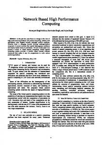
the requested confidence level, then the method of SODA may tend to stop the simulation too late and waste computing resources. We have put this methodology into practice and applied it in fully automated studies of the coverage of selected methods of mean value analysis and quantiles [Pawlikowski et al., 1998a; Lee et al., 1998; Lee et al., 1998a]. The assumed reference set of basic, analytically tractable models used in these analyses included four queueing models (M/M/1, M/D/1, M/H/1 and an open queueing network with a feedback connection). These models were studied under a wide range of traffic intensities and using various numbers of simulation engines. Simulation practitioners know that unusually short simulation runs produce highly unreliable results and, as such, should be rejected. They happen from time to time, since, due the stochastic nature of the processes being simulated, the stopping criteria are sometimes met by chance earlier than they should be. So that the results from unusually short runs did not bias the coverage values obtained, we adopted the following filtering rule: When the required number B of bad confidence intervals is collected, ¯ and standard deviation σ(L) of the simulation run lengths the mean L executed so far should be calculated, and the results from the runs of ¯ − σ(L) should be discarded. length shorter than Lmin = L Such studies are very computationally intensive. For example, in the coverage analysis of one version of the method of Spectral Analysis used for estimating precision of mean values, we conducted simulations of each of the four reference models mentioned above, at nine different traffic levels and using three different numbers of simulation engines. This required executing a total of 108 coverage experiments. Each experiment typically required, on average, about 5000 simulation runs to meet the stopping criteria. Thus, the total number of simulation runs performed during one coverage study of one method of SODA (of many needing to be considered) was over 0.5 million. To manage the considerable volume of data generated by these experiments, we used an Ingres relational database structured as shown in Figure 3. The central, and largest, component of this database is the exprun relation, which contains a tuple for every simulation run, recording the results of that run plus some performance statistics concerning the internal operation of Akaroa2. We kept the results of every run so that we could analyse the results in different ways without having to re-run the experiments, which would have been very time-consuming. We developed automated scripts to extract information from the database and produce plots and tables of coverage and speedup versus selected experimental conditions. These scripts were initially implemented in Tcl [Ousterhout, 1994], and later in Python [van Rossum, 1997].
4
Conclusions
In this paper we discussed main programming issues associated with designing Akaroa2, the newest version of a package for distributed stochastic simulation,
method sim model
exprun
exp anal meth
options
method
#engs
load
run#
results
statistics
expcov methodology
coverage
Fig. 3. Database schema for coverage experiment results.
being developed in the Department of Computer Science at the University of Canterbury in Christchurch, New Zealand. Akaroa2 automatically distributes simulation models (no skills of parallel programming are needed) over a number of computers linked by a local area network, and control the progress of simulation until the required precision of the final results is reached. From the user’s point of view, distributed stochastic simulation in the MRIP scenario appears to be a very attractive application of network computing. It makes good use of the distributed computing power of processors linked by a local area network, significantly speeding up simulation experiments of dynamic stochastic systems regardless of the internal structure of their models, and this is done in a way which remains transparent for users. Our research activities in the project are continuing. They are currently aimed at increasing the functionality of Akaroa2. We are also investigating the possibility of formulating MRIP scenarios in areas of scientific computation other than stochastic simulation.
5
Acknowledgements
Partial financial support for this research has been provided by the University of Canterbury (Grant U6301).
6
References
R. L. Bagrodia (1996). “Perils and Pitfalls of Parallel Discrete Event Simulation”. In Proc. 1994 Winter Simulation Conf. WSC’94, IEEE Press, 1996, pp. 136-143. P. Buchholz et al. (1997). “Report on the Performance Evaluation Techniques and Tools Group”. In Proc. Int. Workshop on System Performance Evaluation Origins and Directions (Schloss Dagstuhl, Germany, Sept. 1997), Int. Research Center for Computer Science, Schloss Dagstuhl, 1997. (See also: http://www.ani.univie.ac.at/dagstuhl97) D. Clark et al. (1996) “Strategic Directions in Networks and Telecommunications”. ACM Computing Surveys (Special Issue on Strategic Directions in Computing Research), 28: 1996, no.4, pp. 679-690. Computer Technology Research Co. (1998). “Network-Centric Computing: Preparing the Enterprise for the Next Millennium”. Strategies and Solutions for the 21st Century, 3, Computer Technology Research Co., USA, 1998.
G. Ewing, D. McNickle and K. Pawlikowski (1997). “Multiple Replications in Parallel: Distributed Generation of Data for Speeding up Quantitative Stochastic Simulation”. In Proc. of 15th IMACS World Congress on Scientific Computation, Modelling and Applied Mathematics, Berlin, August 1997, pp. 379-402. G. Ewing, K. Pawlikowski and D. McNickle (1997a). Akaroa 2.4.2. Technical Report TR-COSC 07/97, Department of Computer Science, University of Canterbury, Christchurch, New Zealand. G. S. Fishman and L. R. Moore III (1986). “An Exhaustive Analysis of Multiplicative Congruential Random Number Generators with Modulus M = 231 − 1”. SIAM J. Sci. Stat. Comput., 7: 1986, pp. 24-45. J. Ousterhout (1994). Tcl and the Tk Toolkit. Addison-Wesley, 1994. K. Pawlikowski (1990). “Steady-State Simulation of Queueing Processes: A Survey of Problems and Solutions”. ACM Computing Surveys, 2: 1990, 123-170. K. Pawlikowski and V. Yau (1992). “An Automatic Partitioning, Runtime Control and Output Analysis Methodology for Massively Parallel Simulations”. In Proc. of the European Simulation Symp. ESS’92, Dresden, 1992, SCS, pp. 135-139. K. Pawlikowski, V. Yau and D. McNickle (1994). “Distributed Stochastic DiscreteEvent Simulation in Parallel Times Streams”. In Proc. of the Winter Simulation Conf. WSC’94, IEEE Press, 1994, pp. 723-730. K. Pawlikowski, G. Ewing and D. McNickle (1998). “Performance Evaluation of Industrial Processes in Computer Network Environments”. In Proc. of European Conf. on Concurrent Engineering ECEC’98, Erlangen, Germany, April 1998, pp. 129-135. K. Pawlikowski, D. McNickle and G. Ewing (1998a). “Coverage of Confidence Intervals in Sequential Steady-State Simulation”. Simulation Practice and Theory, 6: 1998, pp. 255-267. K. Pawlikowski and D. McNickle (1998). “Distributed Stochastic Simulation and Amdalh’s Law”. Submitted. V. J. Rego and V. S. Sunderam (1992). “Experiments in Concurrent Stochastic Simulation: the EcliPSe Paradigm”. J. Parallel and Distributed Computing, 14: 1992, pp. 66-84. G. van Rossum (1997). Python Reference Manual. Corporation for National Research Initiatives (CNRI), 1895 Preston White Drive, Reston, Va 20191, USA. Available from: http://www.python.org Jong-Suk R. Lee, D. McNickle and K.Pawlikowski (1998). “Confidence Interval Estimators for Coverage Analysis in Sequential Steady-state Simulation”. Submitted. Jong-Suk R. Lee, D. McNickle and K.Pawlikowski (1998a). “Sequential Estimation of Quantiles”. Tech. Rep. TR-COSC 03/98, Department of Computer Science, University of Canterbury, Christchurch, New Zealand. V. S. Sunderam and V. J. Rego (1991). “EcliPse: A System for High Performance Concurrent Simulation”. Software-Practise and Experience, 11: 1991, pp. 11891219. V. Yau and K. Pawlikowski (1993). “AKAROA: a Package for Automatic Generation and Process Control of Parallel Stochastic Simulation”. In Proc. 16th Australian Computer Science Conf., Australian Computer Science Comms., 1993, pp. 7182.