cloud computation, algorithm configuration relies on reproducible CPU time measure- ... hardware virtualization on performance measurements (see, e.g., [6â8]).
Algorithm Configuration in the Cloud: A Feasibility Study Daniel Geschwender1 , Frank Hutter2 , Lars Kotthoff3 , Yuri Malitsky3 , Holger H. Hoos4 , and Kevin Leyton-Brown4 1
1
University of Nebraska-Lincoln, 2 University of Freiburg, 3 INSIGHT Centre for Data Analytics, 4 University of British Columbia
Introduction and Related Work
Configuring algorithms automatically to achieve high performance is becoming increasingly relevant and important in many areas of academia and industry. Algorithm configuration methods take a parameterized target algorithm, a performance metric and a set of example data, and aim to find a parameter configuration that performs as well as possible on a given data set. Algorithm configuration systems such as ParamILS [5], GGA [1], irace [2], and SMAC [4] have achieved impressive performance improvements in a broad range of applications. However, these systems often require substantial computational resources to find good configurations. With the advent of cloud computing, these resources are available readily and at moderate cost, offering the promise that these techniques can be applied even more widely. However, the use of cloud computing for algorithm configuration raises two challenges. First, CPU time measurement could be substantially less accurate on virtualized than on physical hardware, producing potentially problematic noise in assessing the performance of target algorithm configurations (particularly relevant when the performance objective is to minimize runtime) and in monitoring the runtime budget of the configuration procedure. Second, by the very nature of the cloud, the physical hardware used for running virtual machines is unknown to the user, and there is no guarantee that the hardware that was used for configuring a target algorithm will also be used to run it, or even that the same hardware will be used throughout the configuration process. Unlike many other applications of cloud computation, algorithm configuration relies on reproducible CPU time measurements; it furthermore involves two distinct phases in which a target algorithm is first configured and then applied and relies on the assumption that performance as measured in the first phase transfers to the second. Previous work has investigated the impact of hardware virtualization on performance measurements (see, e.g., [6–8]). To the best of our knowledge, what follows is the first investigation of the impact of virtualization specifically on the efficacy and reliability of algorithm configuration.
2
Experimental Setup
Our experiments ranged over several algorithm configurators, configuration scenarios and computing infrastructures. Specifically, we ran ParamILS [5] and SMAC [4] to configure Spear [3] and Auto-WEKA [9]. For Spear, the objective was to minimize the runtime on a set of SAT-encoded software verification instances (taken from [3], with the same training/test split of 302 instances each). For Auto-WEKA, the objective
was to minimize misclassification rate on the Semeion dataset (taken from [9], with the same training/test set split of 1116/447 data points). The time limit per target algorithm run (executed during configuration and at test time) was 300 CPU seconds (Spear) and 3600 CPU seconds (Auto-WEKA), respectively. We used the following seven computing infrastructures: – Desktop: a desktop computer with a quad-core Intel Xeon CPU and 6GB memory; – UBC: a research compute cluster at the University of British Columbia, each of whose nodes has two quad-core Intel Xeon CPUs and 16GB of memory; – UCC: a research compute cluster at University College Cork, each of whose nodes has two quad-core Intel Xeon CPUs and 12GB of memory – Azure: the Microsoft Azure cloud, with virtual machine instance type medium (2 cores, 3.5GB memory, $0.12/hour) – EC2-c1: the Amazon EC2 cloud, with virtual machine instance type c1.xlarge (8 cores, 7GB memory, $0.58/hour) – EC2-m1: the Amazon EC2 cloud, with virtual machine instance type m1.medium (1 core, 3.5GB memory, $0.12/hour) – EC2-m3: the Amazon EC2 cloud, with virtual machine instance type m3.2xlarge (8 cores, 30GB memory, $1.00/hour) For each of our two configuration scenarios, we executed eight independent runs (differing only in random seeds) of each of our two configurators on each of these seven infrastructures. Each configuration run was allowed one day of compute time and 2GB of memory (1GB for the configurator and 1GB for the target algorithm) and returned a single configuration, which we then tested on all seven infrastructures. On the larger EC2-c1 and EC2-m3 instances, we performed 4 and 8 independent parallel configuration/test runs, respectively. Thus, compared to EC2-m1, we only had to rent 1/4 and 1/8 of the time on these instances, respectively. This almost canceled out with the higher costs of these machines, leading to roughly identical total costs for each of the machine types: roughly $100 for the 2 · 2 · 8 configuration runs of 24h each, and about another $100 for the testing of configurations from all infrastructures.
3
Results
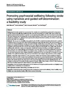
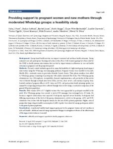
We first summarize the results for the Auto-WEKA scenarios, which are in a sense the “easiest case” for automatic configuration in the cloud: in Auto-WEKA, the runtime of a single target algorithm evaluation only factors into the measured performance if it exceeds the target algorithm time limit of 3600 CPU seconds; i.e., target algorithm evaluations that run faster yield identical results on different infrastructures. Our experiments confirmed this robustness, showing that configurations resulting from configuring on infrastructure X yielded the same performance on other infrastructures Y as on X. While SMAC yielded competitive Auto-WEKA configurations of similar performance on all seven infrastructures (which turned out to test almost identically on other infrastructures), the local search-based configurator ParamILS did not yield meaningful improvements, since Auto-WEKA’s default (and its neighbourhood) consistently led to timeouts without even returning a classifier. We turn to the Spear configuration scenario, which we consider more interesting, because its runtime minimization objective made it less certain whether performance would generalize across different infrastructures. In Figure 1, we visually compare the
100
● ●
100
● ● ●
Desktop
● ● ● ● ●
10
● UBC
UCC Azure ● EC2−c1 ● EC2−m1 ● EC2−m3
● ● ●
●
● ● ●
● ● ● ● ●
● ●
● ● ● ●
100
●
10
configuration performance [CPU s]
● ● ●
Desktop ● ●
10
1 10
● ● ●
● UBC
UCC Azure ● EC2−c1 ● EC2−m1 ● EC2−m3
validation performance [CPU s]
● ●
validation performance [CPU s]
validation performance [CPU s]
● ●
● ● ●● ● ●
● ● ● ● ●
100 ● ● ●
Desktop ● UBC
10
UCC Azure
● ●
● EC2−c1
●
●
EC2−m1
● EC2−m3
● ● ●
100
configuration performance [CPU s]
● ● ● ●
10
100
configuration performance [CPU s]
(a) Configured on UCC (b) Configured on Azure (c) Configured on EC2-m3 Fig. 1. Test performance (log10 runtime) for Spear configurations found in 8 ParamILS runs with different random seeds on 3 different infrastructures. The shapes/colours denote the infrastructure the configuration was tested on. Desktop UBC UCC Azure EC2-c1 EC2-m1 EC2-m3
Desktop
UBC
UCC
Azure
EC2-c1
EC2-m1
EC2-m3
median
0.54 (0.67) 0.07 (0.21) 0.54 (0.51) 0.78 (1.14) 0.53 (0.52) 0.58 (0.99) 0.00 (0.55)
0.52 (0.76) 0.01 (0.11) 0.53 (0.52) 0.78 (1.11) 0.16 (0.51) 0.58 (1.01) -0.02 (0.59)
0.96 (0.46) 0.17 (0.21) 0.56 (0.09) 0.81 (1.03) 0.59 (0.43) 0.59 (0.93) 0.56 (0.51)
0.59 (0.68) 0.22 (0.45) 0.60 (0.07) 0.81 (1.02) 0.58 (0.40) 0.65 (0.92) 0.18 (0.44)
0.59 (0.57) 0.19 (0.18) 0.59 (0.61) 0.81 (1.00) 0.26 (0.41) 0.62 (0.85) 0.30 (0.42)
0.80 (0.62) 0.19 (0.16) 0.58 (0.42) 0.81 (1.01) 0.22 (0.41) 0.62 (0.88) 0.16 (0.46)
0.59 (0.54) 0.15 (0.31) 0.58 (0.42) 0.82 (0.99) 0.55 (0.52) 0.57 (0.89) 0.16 (0.42)
0.59 (0.62) 0.17 (0.21) 0.58 (0.42) 0.81 (1.02) 0.53 (0.43) 0.59 (0.92) 0.16 (0.46)
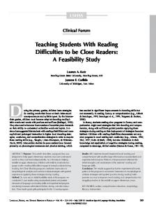
Table 1. Test performance (median of log10 runtimes, and in parentheses, interquartile range) of the 8 Spear-SWV configurations identified by SMAC on the infrastructure in the row, tested on the infrastructure in the column. All numbers are medians of log10 runtimes over 8 runs, rounded to two decimal places. For each test infrastructure, we bold-face the entry for the configuration infrastructure yielding the best performance.
performance achieved by configurations found by ParamILS on three infrastructures. We note that the variance across different seeds of ParamILS was much larger than the variation across infrastructures, and that the performance of configurations found on one infrastructure tended to generalize to others. This was true to a lesser degree when using SMAC as a configurator (data not shown for brevity); SMAC’s performance was quite consistent across seeds (and, in this case, better than the ParamILS runs). Table 1 summarizes results for configuration with SMAC, for each of the 49 pairs of configuration and test infrastructures. Considering the median performance results, we note that configuring on some infrastructures yielded better results than on others, regardless of the test infrastructure. For each pair (X,Y ) of configuration infrastructures, we tested whether it is statistically significantly better to configure on X or on Y , using a Wilcoxon signed-rank test on the 56 paired data points resulting from testing the eight configurations found on X and Y on each of our seven infrastructures. Using a Bonferroni multiple testing correction, we found that UBC and EC2-m3 yielded statistically significantly better performance than most other infrastructures, EC2-c1 performed well, Desktop and UCC performed relatively poorly, and Azure and EC2m1 were significantly worse than most other infrastructures. An equivalent table for ParamILS (not shown for brevity) shows that it did not find configurations as good as those of SMAC within our 1-day budget. Since the variation across configurations dominated the variation due to varying testing platforms, the relative differences across test infrastructures tended to be smaller than in the case of SMAC.
A prime concern with running algorithm configuration in the cloud is the potentially increased variance in algorithm runtimes. We therefore systematically analysed this variance. For each pair of configuration and test infrastructure, we measured test performances of the 8 configurations identified by SMAC and computed their 25% and 75% quantiles (in log10 space). We then took their difference as a measure of variation for this particular pair of configuration and test infrastructure. As Table 1 (numbers in parentheses) shows, configuring on the UBC cluster gave the lowest variation, followed by UCC and the two bigger cloud instances, EC2-c1 and EC2-m3 (all with very similar median variations). Configuring on the Desktop machine led to somewhat higher variation, and configuring on Azure or EC2-m1 to much higher variation. The fact that configuring on the two bigger cloud instances, EC2-c1 and EC2-m3, yielded both strong configurations and relatively low variation suggests that bigger cloud instances are well suited as configuration platforms. As described earlier, their higher cost per hour (compared to smaller cloud instances) is offset by the fact that they allow the parallel execution of several independent parallel configuration runs.
4
Conclusion
We have investigated the suitability of virtualized cloud infrastructure for algorithm configuration. We also explored the related issue of whether configurations found on one machine can be used on a different machine. Our results show that clouds (especially larger cloud instances) are indeed suitable for algorithm configuration, that this approach is affordable (at a cost of about $3 per 1-day configuration run) and that often, configurations identified to perform well on one infrastructure can be used on other infrastructures without significant loss of performance. Acknowledgements The authors were supported by an Amazon Web Services research grant, European Union FP7 grant 284715 (ICON), a DFG Emmy Noether Grant, and Compute Canada.
References 1. Ans´otegui, C., Sellmann, M., Tierney, K.: A gender-based genetic algorithm for the automatic configuration of algorithms. In: CP. pp. 142–157 (2009) 2. Birattari, M., Yuan, Z., Balaprakash, P., St¨utzle, T.: In: Bartz-Beielstein, T., Chiarandini, M., Paquete, L., Preuss, M. (eds.) Empirical Methods for the Analysis of Optimization Algorithms, chap. F-race and iterated F-race: An overview. Springer (2010) 3. Hutter, F., Babi´c, D., Hoos, H.H., Hu, A.J.: Boosting verification by automatic tuning of decision procedures. In: Formal Methods in Computer Aided Design. pp. 27–34 (2007) 4. Hutter, F., Hoos, H.H., Leyton-Brown, K.: Sequential model-based optimization for general algorithm configuration. In: LION-5. pp. 507–523 (2011) 5. Hutter, F., Hoos, H.H., Leyton-Brown, K., St¨utzle, T.: ParamILS: an automatic algorithm configuration framework. J. Artif. Int. Res. 36(1), 267–306 (2009) 6. Kotthoff, L.: Reliability of computational experiments on virtualised hardware. JETAI (2013) 7. Lampe, U., Kieselmann, M., Miede, A., Z¨oller, S., Steinmetz, R.: A tale of millis and nanos: Time measurements in virtual and physical machines. In: Service-Oriented and Cloud Computing. Lecture Notes in Computer Science, vol. 8135, pp. 172–179 (2013) 8. Schad, J., Dittrich, J., Quian´e-Ruiz, J.A.: Runtime measurements in the cloud: Observing, analyzing, and reducing variance. VLDB Endow. 3, 460–471 (Sep 2010) 9. Thornton, C., Hutter, F., Hoos, H.H., Leyton-Brown, K.: Auto-WEKA: Combined selection and hyperparameter optimization of classification algorithms. In: KDD. pp. 847–855 (2013)