A new algorithm for computationally effective calculation of line integrals is pro- ... economical way with fully serial memory access and in practice it proves to be ...... when both are implemented in the C programming language with Microsoft.
Algorithm for Calculation of Discrete X-Ray Transform Ofer Levi and Boris Efros Ben Gurion University of the Negev, Be’er Sheva, Israel Abstract A new algorithm for computationally effective calculation of line integrals is proposed. The algorithm is applicable for both 2D and 3D digital images. The fundamental idea is simultaneous calculation of projections using serial memory access and minimal number of arithmetic operations per coefficient. We compare our algorithm to other known approaches for line integrals computation with respect to various performance measures such as accuracy, speed, and cache coherence. Despite of the fact that the proposed algorithm requires O (n) operations per coefficient, it does so in super economical way with fully serial memory access and in practice it proves to be faster than O (log n) FFT-based algorithms, even for relatively large input arrays, especially in higher dimensions. We also present an iterative solver for the inverse transform as well as dynamic version of the algorithm using a sliding window where the computational cost of the updates is O (1) per coefficient. We focus our discussion on the 2D case and explain how it can be generalized to higher dimensions.
1
Introduction
Numerous applications require fast and exact calculation of line integrals over a set of lines with various orientations and locations. Among such applications are edge and ridge detection [11], curve extraction, filamentary structures identification [8] as well as reconstruction from projections [16]. The Mathematical operator that transforms input spatial data into the parametric space of line integrals is called the X-Ray Transform [18]. In 2D, the X-ray transform is also known as Radon and Hough Transforms [13]. Another related transform is the Beamlet Transform [9], a multiscale version of the X-Ray transform, which requires calculation of line integrals at various scales and not only for a single global scale. Due to recent rise of 3D and higher dimensional image analysis methods in Medical Imaging, Infrared Vision and other application fields, fast calculation of line integrals is highly important for processing of data which may contain structures built of line segments and filaments. Additionally, 3D mono-scale and multiscale line-integral transforms can be used successfully in multiframe target detection [17] and Geometric Analysis of point clouds in 2D, 3D as well as in higher dimensions [10]. We believe that, the variety of prospective applications over a wide range of fields is much wider, especially for the multiscale approach [2].
1
1.1
Contents
The contents of the paper are as follows: • The introductory section is devoted to important factors for the discrete X-ray transform implementation and survey of existing techniques • Section 2 contains description of suggested algorithms (static and dynamic). • Section 3 exhibits some performance comparisons. • Section 4 is devoted for summary, discussion, and future work challenges.
1.2
From Continues to Discrete
In the continuum, the X-ray transform of a function f (x, y) with (x, y) ∈ R2 takes the form R (Xf )(L) = L f (p)dp , where L is a line in R2 and p is a variable indexing point on the line; hence, the mapping f 7→ Xf contains within it all line integrals over f . In the discrete case, the X-ray transform is not uniquely defined. The definition of both: discrete input (digital image) and discrete output (integrals over finite set of lines) needs to be carefully defined. A digital image I[i, j] is a representation of a two-dimensional function as an array of digital values,called pixels. A pixel at the position (i, j) is representing square region [i − l, i] × [j − l, j]. In other words, digital image is generated by a sampled 2D function. In the discrete case line integral takes the form of a simple weighted sum X (Xf )(l) = f (i, j) · wij (l) (1) i,j
This form is the natural discrete adaptation of continues version, which also preserves linearity properties. The integral obtains the form of weighted sum, when the weights are distributed along the corresponding line. The function f (x, y) can be seen as a piecewise constant interpolation of the sample points I[i, j] , see Equation 2; or as a result of a smoother interpolation scheme as shown in 3. f (x, y) = f [i, j],
i ≤ x < i + 1, j ≤ x < j + 1 ½ f [i, j], x = i, y = j fˆ(x, y) = I(x, y, f ), else
(2) (3)
According to the first definition,wij = |Lij | – is the length of intersection between line and pixel. This interpolation scheme is very widely used, especially in the domain of the Image Processing. One of the reasons for it, beside the simplicity, is the consistency with image visualization on screen. For the interpolation scheme 3, the meaning of line integrals depends on the chosen interpolation method, an example is shown in the Section 3.1. To implement a digital X-ray transform one needs to define finite parameterized system of lines. The choice of such a family mostly depends on compactness, invertability and requirements of the end-user application. Comprehensive viewpoints on ‘digital geometry’ and ‘discrete lines’ can be found in [15]. 2
1.3
Performance Measures
Number of performance measures should be taken into account when considering a discrete X-ray transform - accuracy, speed, flexibility 1 of line set parameterization and invertability of the entire transformation. As soon as an algorithm is about to be implemented by software, the following measures should also be considered: computational robustness [7] and cache awareness such as sequential memory access and in-place implementations [14]. The aspect of cache awareness may even be critical for the software when dealing with high-dimensional image processing due to large amount of involved data. The fact that the computer memory can be actually viewed as a 1D array should be always kept in mind(for this reason neighbor picture or volume elements in the image are not necessarily neighbors in the computer memory).
1.4
Survey of digital X-Ray Transforms Algorithms
Once a discrete X-ray transform is defined the appropriate algorithm for its calculation should be designed taking into account all performance measures mentioned above. Consider the input as square image with integer side size n. We include in our survey three different approaches for implementation of the discrete X-Ray transform: Direct Evaluation, TwoScale Recursion, and Fast Slant-Stack. Direct Evaluation is an obvious algorithm for computing the X-ray coefficients: one at a time, it simply computes the sums underlying the defining integrals. This algorithm steps systematically through the system of lines, identifies the pixels on the path for each line, visits each pixel and forms a weighted sum of the pixel values where the weights are the lengths of the intersection of each pixel with the given line. The straightforward way to do this is explicitly tracing each line from pixel to pixel and calculating the arc length of the line fragments within each pixel. Doing so is inelegant and computation-wise inefficient. Theoretically, its computation time is O(n) operations per coefficient. Two main advantages of the approach are exactness and flexibility in lines parameterization. The algorithms of the so-called Two-Scale Recursion type are asymptotically much faster, they are based on an idea which has been well-established in the two dimensional case [6, 5, 11]. The extension for 3D transform can be found in [9]. This type of algorithms is based on the divide-and-conquer principle. Generally, each line segment at the coarse scale can be approximated by final number of line segments at the next finer scale [9], see Figure 1. We can use this fact to work systematically from fine scales to coarse scales. In this way line integrals for the coarse scale can be computed by combining X-ray coefficients from the next finer scale. The results are never exact, and in order to increase the level of accuracy one must apply oversampling or accurate and expensive interpolation. Despite of the theoretical O(log n) computational time per coefficient, in practice the running time is much slower because of the required non-sequential access to the coefficients space which is much bigger than the image space especially in higher dimensions. 1
Especially significant in the case of synthesis when the set of lines of the transform needs to be adjusted to the given data.
3
Figure 1: The approximation of line segment L0 (dashed) with usage of 3 segments in next finer scale (dotted).(Xf )(L0 ) ≈ (Xf )(L1 ) + (Xf )(L2 ) + (Xf )(L3 ) Averbuch et al. [3] developed the Fast Slant Stack Algorithm (FSS) which computes a discrete 2D Radon Transform. This algorithm is based on a discrete Projection-Slice Theorem that relates between the X-ray and Fourier space. See Figure 2.
Figure 2: The Relations between the Fourier, Radon, and Real space according to the Projection Slice Theorem. The Fast Slant Stack Algorithm uses a nearly polar fast an exact Fourier Transform called the Pseudo-Polar FFT. Applying a series of inverse 1D FFT’s along the radial lines of the Pseudo-Polar grid produces the Slant Stack coefficients. For this grid, the Fourier coefficients can be computed exactly in O(log n) flops per coefficient. However, it should be mentioned that the constant multiplier of the complexity base function is rather large due to numerous complex calculations involved. It is important to mention that the X-ray coefficients generated by the fast slant stack transform correspond to a family of lines that are equally sampled with respect to their slopes and not with respect to their angles, and that the uniform spacing of lines in each projection varies with respect to the slope, which is not the natural choice and might be problematic. The Fast Slant Stack algorithm can be generalized to 3D in several ways. One of the 4
approaches [9] combines the 2D Fast Slant Stack with the operation of 3D shearing. As for accuracy, the result of each line integral generated by the fast slant stack algorithm is equivalent to integrating over a trigonometric interpolation of the digital image. As a result, high percentage of the total weight involved in a line integral calculation is dispersed over the pixels, which are disjoint from the line as will be shown in Section 3.1. Due to high accuracy and speed, we consider the FSS algorithm superior over the other approaches mentioned above. Hence, we will use the FSS as a benchmark for evaluating the performance of our proposed new algorithm.
2
The SHAS Algorithm
For the sake of simplicity, we concentrate on the two-dimensional case, whereas the extension to algorithms for higher dimensions and implementations results will be discussed. Our algorithm views the input image as a piecewise constant function. Initially, we describe the system of lines used for evaluation of our algorithm. The proposed algorithm and its variants with respect to the initial choice of lines system will be presented.
2.1
System of Lines
Our algorithm is flexible with respect to the choice of slopes of the discrete lines set. However, we will focus our discussion on the family of lines defined by a parameterization called SlopeIntercept System [9]. This is exactly the same system as used for the Slant Stack Algorithm. Therefore, our results can further serve for algorithms comparison. For this family, it is better to translate the center of mass of the cube to be in the origin (0, 0) . Hence, for the (x, y) in the data cube, we have |x|, |y| ≤ n2 . We can consider two families of lines X-driven and Y -driven, depending which axis provides the shallowest slopes. X-driven line takes the form: y = sy x + ty
(4)
with slope sy , and intercept ty . Here, the absolute values of slopes are less than 1 which makes slopes discretization over the entire orientation range possible. We will consider the family of lines generated by this, where the slopes and intercepts run through the equispaced family: sy ∈ {2i/n, i = −n/2, . . . , n/2 − 1} ,
ty ∈ {2i/n, i = −n + 1, . . . , n − 1}
(5)
Y -driven lines are defined with an interchange of the roles between axes, see Figure 3.
2.2
Overall strategy
As mentioned in Section 1.2, the algorithm of Direct Evaluation can be successfully used for computing line integrals by presenting them as weighted sums of pixels’ intensities. We will show how to significantly speed up the computations using the following properties of our line set: 5
Figure 3: X-driven and Y-driven sets of lines with zero intercepts. 1. The weights distribution over parallel lines are identical. 2. There exist an efficient algorithm for deriving a weights vector for each given line orientation. 3. The entire set of X-ray coefficients over equally spaced parallel set of lines (a single projection) can be computed in batch using serial memory access. Let us consider an X-driven line segment L with zero-intercept, i.e. tx = 0 . Suppose it is connecting two integer grid points (oX , oY ) and (dX , dY ) , and passes through the origin then dX = n/2 oX = −n/2
dY = sX · n/2 oY = −dY
(6)
Notice that the line segment intersects with X-grid line each kLk2 /|∆x| units and with Y -grid line each kLk2 /|∆y|, where kLk2 denotes the segment’s length and ∆x and ∆y are defined as follows: ∆x = dX − oX
∆y = |dY − oY |
(7)
We use the term ‘fragment’ to describe a line sub-segment bounded by two neighbor grid-lines (intersection of a given line with a pixel). Consider a set of X-driven lines with the same slope; the underlying strategy in our algorithm is batch computation of the entire set of corresponding line integrals by serial processing of fragments and adding the contribution of each column for all calculated coefficients. For illustration purpose, we consider a line that connects two grid points. We are interested in retrieving the information regarding the sequence of pixels it traverses and the proportions of the segment length inside each such pixel. Figure 4(a) presents an example of line that connects the boundary grid points o = (−4, −3) and d = (4, 3) of a data cube with side length n = 8 . It is divided by grid lines into 12 fragments. Let Ψ be an array of size m × 3 that contains information about fragments, where m is the number of fragments inside the original line segment. Within one column, an Xdriven line can intersect with a Y -grid-line at most once, hence m ≤ 2n. The value Ψ∆ (i) corresponds to the proportional length of the i-th fragment, whereas ΨX (i) and ΨY (i) are boolean indicators that equal one if the i-th fragment is bounded from the left by the 6
Figure 4: Illustration of the equivalence of weights distribution for parallel lines. HH
HH i 1 Ψ HH
Ψ∆ (i) ΨX (i) ΨY (i)
2
3
4
5
6
7
8
9
10
11
12
1/8
1/24
1/12
1/12
1/24
1/8
1/8
1/24
1/12
1/12
1/24
1/8
1 1
1 0
0 1
1 0
0 1
1 0
1 1
1 0
0 1
1 0
0 1
1 0
Table 1: Line fragments array of line segment with edges (-4,-3) and (4,3). corresponding grid line and zero otherwise. We term this array ‘Ψ - line fragments array’. Clearly, each set of lines with the same slopes sX are associated with the same line fragments array Ψ = Ψ (sX ) regardless of the intercepts values. The intercept difference of any line within the set is reflected by vertical shift of fragments with respect to the zero-intercept line which is never larger than n/2, see Figure 4. The observation that we made earlier provides us with an easy and elegant method for evaluating the structure Ψ by merging two series of interval lengths (or more for higher dimensions). Figure 5 visualizes this method and Table 1 contains the line fragments for the line in our example.
Figure 5: Illustration of efficient calculation of the line fragments array by series merging. The integral over the line segment from our example can be directly computed using the following expression: (Xf ) (L) = ¡ ¢ = 1/8 · f (−4, −3) + 1/24 · f (−3, −3) + 1/12 · f (−3, −2) + · · · + 1/8 · f (3, 2) · kLk2 Ψ∆ (i) is a multiplier of the i-th sum-member, whereas ΨX (i), ΨY (i) are used to easily increment indexes 2 . Generally, we can express this as: 2
The pixel coordinate in this example is in the lower left corner
7
Xf L = kLk2 ·
m X
³ ´ ˆ X (i) , Ψ ˆ Y (i) Ψ∆ (i) · f Ψ
(8)
i=1
where ˆ X (i) = oX + Ψ
i X
ΨX (j)
ˆ Y (i) = oY + sign(dY − oY ) · Ψ
j=2
and
i X
ΨY (j)
(9)
j=2
q q kLk2 = (dX − oX )2 + (dY − oY )2 = n s2X + 1
(10)
Traversing the line fragments array provide an easy and coherent way for summing all necessary and properly weighted pixels for exact computation of the line integrals. Until now, we referred only to lines with zero intercepts; the only difference in the computation of nonzero intercepts coefficients is that the indices of the appropriate pixels should be shifted in the Y direction by integer values according to their intercepts. These shifts are constant through all X coordinates for each projection. Therefore, we can calculate an entire projection by traversing through its line slices array, applying a shift to the whole data slice for each X coordinate in the Y direction and adding the contribution of this slice to the³resulting vector ´ ˆ X (i) , Ψ ˆ Y (i) of size 2n . Shifts are performed in such a way that a pixel at position Ψ ³ ´ ˆ X (i) , 0 . We call our algorithm Shift-And-Sum (or SHAS ), is ‘moving’ to the position Ψ since these two operations are the most dominant in our algorithm.
2.3
The Algorithm
The algorithm input is a 2D data array f [x, y] ∈ Rn×n . The output is an array of the resulting coefficients of the X-ray transform over the appropriate set of lines:Xf [η, s, t] ∈ R2×n×2n . The parameter η is used as an index for the line-family (X or Y -driven), s is the slope index and t is the intercept index. We use the notation Ψs for the Line Fragments Array. This array is exactly the same for X- and Y -driven line segments. Let E be the operator of extension by padding an array n wide and n tall to be n wide and 2n tall by adding extra rows of zeros symmetrically above and below the input argument. Let I˜ = EI. Let S be the shift operator over vectors of size 2n, then S d is the d-positions shift operator. Given any vector v ∈ R2n , the result of S d v for any integer d is a vector w ∈ R2n , where the i-th element of v is identical to the element at position (i + d) in w or zero if index (i + d) exceeds matrix dimensions. The procedure for the X-ray transform of a 2D digital image is following. Algorithm 2.1 Input: f [x, y] Output: Xf [η, s, t] 1: for all line type η ∈ X − driven, Y − driven do 2: for all slope s do 8
3: 4: 5: 6: 7:
Derive Ψ = Ψs , m is the number of rows ³ inΨ h i´ Pm ˆ Y (i) ˜ −Ψ ˆ X (i), : Xf [η, s, :] = klk2 · i=1 Ψ∆ (i) · S If Ψ Transpose the input array end for end for
2.4
SHAS Algorithm in Higher Dimensions
The extension to higher dimensions is straight forward. One should notice that in 2D we have X : R2 � R2 , but in general X : Rd � R2(d−1) . The so-called ‘curse of dimensionality’ is reflected here by fact that we need (d − 1) slope and intercept pairs to define line in Rd , as we consider d groups of lines by shallowest slope. For example, X,Y and Z-driven in R3 (see Figure 6). Line Fragments Array Ψ(s1 , . . . , sd−1 ) will contain d rows, but still m = O(n) columns. The above algorithm for the d-dimensional case requires extension of circular shift operator for arrays in Rd−1 .
Figure 6: The domains of X, Y and Z-driven lines. Due to the practical importance of the 3D version of the algorithm, we provide the 3D SHAS Algorithm A.1 in the Appendix A.1.
2.5
Dynamic SHAS Algorithm
The nature of the SHAS algorithm invites the extension for dynamic applications with realtime input updates. Consider a sliding window of size n × n that can slide in any direction X or Y and occupies consecutive regions of 2D image (“Step Right / Left / Up / Down”). We will present a modification of the SHAS algorithm, which is used for dynamic update of all n2 X-ray coefficients for the sliding window in only O(n2 ) time for a single position shift. Our intention is to stay with the same lines system even after the shift of the window and perform only minor updates for each line-segment, preserving principles of robust and effective calculations. We first discuss “Step Right” circumstances. We denote by ∆X (s) a zero-intercept offset of the smallest Y distance between X-driven line segment with slope(s) and the origin, ∆Y (s) is defined similarly for the second dimension. For the X-driven lines, we need to recalculate zero-intercept offset for each slope. Due to the equispaced sampling of lines we can ensure that its absolute value will never be higher than 0.5 by performing a shift of 1 if needed. Moreover, for any slope there exist ns such that ∆x (s) = 0 each ns steps, when ns is a divider of n/2 . 9
The shift of the center of mass brings about the possible shift of all output coefficients’ intercept. Due to the definition of the X-driven lines, the magnitude of the shift is never higher than 1 and depends only on the slope. In order to preserve nearly the same system of lines, the shift of the output coefficients is performed.
Figure 7: The illustrative presentation for updating the X-driven coefficients. The window is sliding in the X-direction. Panel A illustrates the changes in the zero-intercept offset. Panel B illustrates the distribution of weights over not more than two adjacent pixels. The output shift is ±1 or 0, depends on slope. The dynamic update procedure is different for X-driven (slopes in the range [−1; 1] ) and Y -driven lines (absolute value of slopes higher than 1). The main reason for this is illustratively presented and explained in Figures 7, 8. The algorithm 2.2 takes care for the X-driven lines updates, each coefficient is updated with finite number of operations (less than 2). Whereas for Y -driven set some coefficients may require up to n operations, they are compensated by set of coefficients, that will require only re-indexing. The order of update operations is the same for both sets. Algorithm 2.2 Notations: Xf 0 = Xf 0 (s, t)- Input 2D array of the current X-ray coefficients Xf = Xf (s, t)- Output 2D array of updated X-ray coefficients ∆0x = ∆0x (s)- Input vector of current zero-intercept offsets of X-driven lines ∆x = ∆0x (s) - Output vector of updated zero-intercept offsets of X-driven lines v in = v in (t)- Updated row v out = v out (t)- Outdated row Input: Xf 0 , ∆0X , vin , vout Output: Xf, ∆X 1: η = X 2: for all slope s do 3: ∆(s) = slope(s) + ∆0X (s) if ∆(s) ∈ (0.5, 1.5] then 4: 5: offset = 1 else if ∆(s) ∈ [−1.5, 0.5) then 6: 10
7: 8: 9: 10: 11: 12: 13: 14: 15:
offset = −1 else offset = 0 end if ∆X (s) = ∆0X (s) + offset ˆ X , w1 for the row v out FindΨ ³ ³ ´ ³ ´´ ˆ ˜ out − (1 − w1 )S Ψˆ Y +sign(slope(s)) Iv ˜ out kLk2 Xf (s, :) = Xf 0 (s, :) − w1 S ΨY Iv ˆ X , w1 for the row v in FindΨ ´ ³ ´´ ³ ³ ˆ ˜ in − (1 − w )S Ψˆ Y +sign(slope(s)) Iv ˜ in kLk Xf (s, :) = S offset ·X 0 f (s, :)− w S ΨY Iv 1
1
2
16: end for
Figure 8: The illustrative presentation for updating the Y-driven coefficients. The window is sliding in the X-direction. The magnification emphases how the indexes of coefficients in projection and columns in vin (or vout ) are found for any index i in array Ψ . Zero-intercept offset does not change. The output shift is always ±1 . The algorithm for updating Y -driven lines is based on the reduction of SHAS algorithm (see Figure 8).The pseudo-code for it is found in the Appendix A.2. Apparently, the procedure for ‘Step Left’ is the same as ‘Step Right’ after turning upside down the order of slopes and column vectors v in , v out . The procedures for ‘Step Up’ and ‘Step Down’ are like ‘Step Right’ and ‘Step Left’ then the X-driven lines are updated with Y -driven procedure and vice versa.
2.6
Software Implementation Remarks
The implementation of the above algorithms is quite straightforward and effortless. It should be noticed that there is no need for the zero-padding operation in practice; we only need to know the new coordinates of the lowest left data array corner after shift operations to perform correct summation. Therefore, each summation requires only n operations instead of 2n as it may seem from Algorithm 2.1. The act of switching lines family is transpose–like
11
operation, but it can be performed by relabeling of axes 3 in O(1) flops. Another step toward fast implementation is using the symmetry of Line fragments array and rearranging data cube such that the i-th slice will be adjacent to (n − i)-th slice. Due to the structure of the algorithm, it is natural to think of a parallel implementation in order to speed up the calculations. Any set of X-ray coefficients with the same slopes can be computed independently on separate processing unit. We prefer to omit some technical details and remarks for practical implementation of these algorithms. Efficient software implementations of 2D and 3D monoscale and multiscale versions of these algorithms are freely available for research proposes at [1].
2.7
Adjoint and Inverse Transforms
The SHAS algorithm is a linear operator, each coefficient can be expressed by inner product of pixel intensities and appropriate weights. Therefore, if we present an input image as a column vector x and the SHAS transform operator as a matrix W we simply get y = W x where the output X-ray coefficients is a column vector y. Theoretically, W can be constructed during the algorithm run, but this would be impractical due to the matrix size and inefficient since A is very sparse. The adjoint of the X-ray transform (W T ) is a very useful operator.For the X-ray transform related to SHAS algorithm, the corresponding adjoint can be computed using very similar ideas as the ones used for applying the forward transform, and with comparable computational complexity. While the X-ray transform maps pixel arrays into X-ray coefficient arrays, the adjoint transform maps X-ray coefficient arrays into pixel arrays.
Figure 9: Convergence rate of the iterative inverse transform for different image sizes When the adjoint operator is applied to a coefficient array filled with zeros except for a single positive value, the result is a pixel array where the non-zeros weights are distributed 3
For high dimensions data reorganization should be performed to ensure serial data access
12
along a ‘geometrically correct’ line, corresponding to the location of the non-zero coefficient, Figure 10 illustrates this. The convergence rate of an iterative inverse transform based on the Conjugate Gradient method [12] for solving the Least Square Problem is shown in Figure 9. The number of iterations depends on both data size and required accuracy. For experimenting the iterative inverse we used random square images of various sizes; axis X stands for number of iterations, whereas axis Y is the ratio between norms L2 of the error and the original image. Each plot shows the result for a different image size. We used 1% relative norm of the square error as stopping criteria.
3
Performance
We consider all of the key performance measures for the SHAS algorithm mentioned above (see Section 1.3). The summary of the main properties as compared to other algorithms is found in Table 2, further explanations are included in the following sub–chapters.
Exactness Run Time per coefficient Memory Access Memory Space Complexity Flexibility
3.1
Table 2: Summary of X-ray algorithms main properties. Direct Recursive Fast Slant SHAS Evaluation Approximations Stack Piecewise No Geometric Piecewise constant Interpolation constant O(n) O(log n) O(log n) with O(n) with high constant low confactor stant factor Not serial Not serial Serial Serial O(n3 )
O(n4 )
O(n3 )
O(n3 )
Very high
Low
Low
High
Accuracy and Robustness
The SHAS algorithm computes exact values for the X-Ray transform over the set of lines defined above, where a digital image is viewed as a piecewise constant function, i.e. each picture element is associated with a constant intensity. This is illustrated in Figure 10, where we present the results of the SHAS-based X-Ray transform adjoint operator (top row). For comparison, similar results of the 2D Fast Slant Stack adjoint operator [3] are presented in the bottom row. Due to [3] the results of the Slant Stack algorithm are equivalent to the sum
13
Figure 10: These images show the weights involved in the calculations of various coefficients. SHAS - top row; Fast Slant Stack - bottom row.
n/2−1
SS(y = sx + t, f ) =
X
fˆ(u, su + t)
(11)
u=−n/2
Using the interpolation n/2−1
fˆ(u, y) =
X
f (u, v)D2n (y − v)
(12)
u=−n/2
With the Dirichlet kernel Dl = eiπt/l ·
sin(πt) l · sin(πt/l)
(13)
Thus, the distribution of the non-zero weights involved in the calculation of a given coefficient can include non-zero weights to pixels that are distant from the corresponding line. These artifacts will not be present only for lines which are composed of only one fragment per column, such as strictly horizontal, vertical or diagonal lines (see Figure 10). Furthermore, using only simple arithmetic operations such as summation and multiplication over the real numbers assures computational efficiency and robustness. This fact helps avoiding any inconsistencies such as negative output coefficients, even for positive inputs which is unavoidable in the Slant Stack transform.
3.2
Timing Comparison
The theoretical complexity of floating point operations required for calculation of a single coefficient for an image of size n by n is O(n) in the SHAS algorithm and only O(log n) in the Slant-Stack algorithm. Therefore, we are not expecting these algorithms to compete for very large image size, asymptotically the Slant Stack is faster. However, the SlantStack algorithm involves the application of the fractional Fourier Transform, which is more expensive than a standard FFT [4]. For this reason, the constant multiplier for the actual 14
number of operations can be quite large. On the other hand, the multiplier of the SHAS algorithm is about 2 and the involved operations are summation and multiplications of real numbers only. Therefore, the SHAS algorithm is faster than the FSS for small to medium image sizes. Figure 11 presents a comparison between the 3D Slant Stack and the 3D SHAS algorithms when both are implemented in the C programming language with Microsoft Visual C++ .NET compiler using double precision. Tests were performed on a Pentium 4 PC, 2.4GHz, and 512 Mb of RAM. It can be seen that the FSS algorithm running time is not monotonously non-decreasing throughout the entire range of image size as expected, this inconsistency with the theoretical complexity is probably caused by the sensitivity of the FFT implementation for the input sizes.
Figure 11: Timing Comparison. These experimental results verify that the SHAS algorithm is significantly more effective than the Slant Stack even for relatively large 3D images.
3.3
Compatibility with cache memory
One of the most important advantages of the SHAS algorithm is its cache-awareness, i.e. it is very well-organized for use with modern hierarchical memory computers [14]. When a big data structures such as typical 3D images are being processed, non-serial data access can result in many cash-misses (CPU memory overflow) and page-faults (process virtual memory overflow). Serial data access is the key to bring the number of such unwanted events to minimum. This is well achieved in the SHAS algorithm, because each image slice occupies separate continuous memory block.
3.4
Flexibility with Respect to the Couch of Line Set
Unlike the FSS Algorithm, the SHAS algorithm allows some flexibility with respect to the choice of line set, the basic requirement of the SHAS algorithm is that the set of lines will consist of subsets of parallel equispaced lines with integer vertical or horizontal shifts in the 15
basically vertical or basically horizontal sets respectively. No constraints on slopes have to be made. The slopes density and angular spacing do not influence the algorithm effectiveness and can be arbitrary. On the other hand, the Slant Stack Algorithm is restricted to the pseudo-polar grid in the frequency domain. The family of lines used in the Slant Stack transform must be equally sloped.
4
Summary and Discussion
A new efficient algorithm for exact computation of line integrals in multi-dimensional image over a special parametric set of lines is introduced. The numerical experiments for relatively bid image sizes prove that the algorithm is competitive with the fastest X-ray transform algorithms. This efficiency is achieved due to batch computation using a highly economical approach and serial data access. We expect this algorithm to be especially useful for the multiscale transforms, such as the beamlet transform. It seems that great benefit in both speed and accuracy can be achieved by fusion of the X-ray algorithms. For example, the exact calculations of line integrals over the fine scales can be performed using the SHAS algorithm and then two-scale recursion or Slant-Stack can be involved for the calculations of the coarser scales. The algorithm can be easily generalized for higher dimensions of input data and is well suited for parallel implementations. Any set of X-ray coefficients with the same slopes can be computed independently on separate processing unit.
Figure 12: Demonstration of the application of RT filament following in 3D The dynamic version of the X-ray transform over a sliding window is introduced as well. Beside of exactness and robustness the dynamic SHAS algorithm has optimal running time in terms of the output size. This fact makes it perfectly suitable for real time applications, for example in surveillance systems or in medical imaging applications with dynamic region of interest. Figure 13 illustrates a 2D RT application for detection of line segments buried in noise. Figure 12 contains screen-shots of the RT application for filament tracing in 3D.
16
Figure 13: The SHAS algorithm, which implements the Radon transform over a sliding window is applied in real time. The line segment detection is based on simple run-length test. The only assumption used is that the underlying noiseless image can suffer only slight changes in time proportional to the overlaying window size.
A A.1
Appendices The SHAS Algorithm for 3D Input
The procedure for the X-ray transform of 3D data follows: Algorithm A.1 Notations: f [x, y, z] ∈ Rn×n×n – input 3-D voxel array Xf [η, s1 , s2 , t1 , t2 ] ∈ R3×n×n×2n×2n – output 5-D coefficients array. η - index for the line’s type (X, Y or Z-driven) s1 ,s2 ,t1 ,t2 - pair of line slopes and pair of line intercepts indices Ψsx ,sy - line fragments array for Z-driven lines with slopes sx , sy . I˜r = EI and I˜c = IE 0 – are the identity matrices of size n, padded by extra rows or columns of zeros respectively. Input: f [x, y, z] Output: Xf [η, sX , sY , tX , tY ] 1: for all line type η ∈ X − driven, Y − driven, Z − driven do 2: η=Z 3: for all pair of slopes sX , sY do 4: Derive Ψ = ΨsX ,sY 17
³ h i ´³ ´0 P ˆ X (i) ˜ −Ψ ˆ Z (i), :, : I˜C S −Ψˆ Y (i) Xf [η, s, :] = kLk2 · m Ψ (i) · S I f Ψ ∆ Y i=1 6: end for 7: Change grids roles:Z → Y, Y → X, X → Z (Transpose) 8: end for 5:
A.2
DSHAS for Y-Driven lines set
Algorithm A.2 Input: Xf 0 , ∆0Y , vin , vout Output: Xf, ∆Y 1: η = Y 2: for all slope s do 3: ∆(s) = slope(s) + ∆0X (s) 4: ∆Y (s) = ∆0Y (s) + 1 5: DeriveΨ = Ψs , m is the number of rows in Ψ 6: for all 1 ≤ i ≤ m do 7:
h i h i ³ h i´ ˆ Y (i) = Xf η, s, n/2 − Ψ ˆ Y (i) − klk2 · Ψ∆ (i) · v out Ψ ˆ X (i) Xf η, s, n/2 − Ψ 8: 9: 10: 11:
end for Xf [η, s, :] = S −1 Xf [η, s, :] for all 1 ≤ i ≤ m do h i h i ³ h i´ in ˆ ˆ ˆ Xf η, s, 3n/2 − ΨY (i) = Xf η, s, 3n/2 − ΨY (i) + klk2 · Ψ∆ (i) · v ΨX (i)
end for 12: 13: end for
18
References [1] Shas software. http://www.bgu.ac.il/ efros/research.html. [2] E. Arias-Castro, D. L. Donoho, and X. Huo. Near-optimal detection of geometric objects by fast multiscale methods. IEEE Trans. Inf. Theory, 51(4):2402–2425, 2005. [3] A. Averbuch, R. R. Coifman, D. L. Donoho, M. Israeli, and J. Walden. Fast slant stack: A notion of radon transform for data in a cartesian grid which is rapidly computable, algebraically exact, geometrically faithful and invertible. Tech. Rep. (preprint), 2001. httt://ww.math.tau.ac.il/amirl/. [4] D. H. Bailey and P. N. Swarztrauber. Fast fractional fourier transforms and applications. SIAM Review, 33:389–404, 1991. [5] M. L. Brady. A fast discrete approximation algorithm for the radon transform. SIAM J. Computing, 27(1):107–119, 1998. [6] A. Brandt and J. Dym. Fast calculation of multiple line integrals. SIAM Journal of Scientific Computing, 20(4):1417–1429, 1999. [7] M. de Berg, M. van Kreveld, O. Overmars, and O. Schwarzkopf. Computational Geometry - Algorithms and Applications. Springer–Verlag, Berlin, 1997. [8] D. Donoho and X. Huo. Beamlet pyramids: A new form of multiresolution analysis, suited for extracting lines, curves, and objects from very noisy image data. Proceedings of SPIE, 4119:434–444, 2000. [9] D. Donoho and O. Levi. Fast x-ray and beamlet transforms for three-dimensional data. Technical report, Dept. of Statistics, Stanford University, Stanford, California, 1999. [10] D. Donoho, O.Levi, J. Starck, and V. J. Martinez. Multiscale geometric analysis for 3-d catalogues. in AstronomicalData Analysis II, Proceedings of SPIE, 4847:101–11, August 2002. Waikoloa, Hawaii, USA. [11] J. Dym. Multilevel Methods for Early Vision. PhD thesis, Weizmann Institute of Science, Rehovot, Israel, 1994. [12] G. Golub and van Loan. Matrix Computations. Johns Hopkins University Press, Baltimore, 1983. [13] W. A. Gˇotze and H. J. Druckm¨ uller. A fast digital radon transform - an efficient means for evaluating the hough transform. Pattern Recognition, 28(12):1985–1992, 1995. [14] J. L. Hennessy and D. A. Patterson. Computer Architecture: A Quantitative Approach. Morgan Kaufmann Publishers, San Francisco, CA, 2 edition, 1996. [15] G. Herman. Geometry of Digital Spaces. Birkhauser, Boston, 1998.
19
[16] T. Herman. Image Reconstruction From Projections: The Fundamentals of Computerized Tomography. Academic Press, New York, 1980. [17] B. Porat and B. Friedlander. A frequency domain algorithm for multiframe detection and estimation of dim targets. IEEE Transactions Pattern Analysis and Machine Intelligence, 12(4):398–401, 1990. [18] D. Solmon. The x-ray transform. Journal of Mathematical Analysis and Applications, 56:61–83, 1976.
20