Journal of Modern Applied Statistical Methods May 2016, Vol. 15, No. 1, 884-892.
Copyright © 2016 JMASM, Inc. ISSN 1538 − 9472
JMASM Algorithms and Code
Algorithm for Combining Robust and Bootstrap In Multiple Linear Model Regression (SAS) Wan Muhamad Amir
Mohamad Shafiq
Hanafi A. Rahim
University of Science, Malaysia Kelantan, Malaysia
University of Science, Malaysia Kelantan, Malaysia
University Malaysia Terengganu Kuala Terengganu, Malaysia
Puspa Liza
Azlida Aleng
Zailani Abdullah
Universiti Sultan Zainal Abidin Kuala Terengganu, Malaysia
University Malaysia Terengganu Kuala Terengganu, Malaysia
University Malaysia Kelantan Kelantan, Malaysia
The aim of bootstrapping is to approximate the sampling distribution of some estimator. An algorithm for combining method is given in SAS, along with applications and visualizations. Keywords:
Multiple linear regression, robust regression and bootstrap method
Introduction Multiple linear regression (MLR) is an extension of simple linear regression. Table 1 displays the data for multiple linear regression. Table 1. Data template for multiple linear regression i 1 2 ⋮ n
yi y1 y2
xi0 1 1
xi1 x11 x21
xi2 x12 x22
⋮
⋮
⋮
⋮
yn
1
xn1
xn2
… … …
xip x1p x2p
…
xnp
⋮
Dr. Amir bin W Ahmad is an Associate Professor of Biostatistics. Email him at:
[email protected]. Mohamad Shafiq Bin Mohd Ibrahim is a postgraduate student in the School of Dental Sciences. Email him at:
[email protected].
884
AMIR ET AL
MLR is used when there are two or more independent variables where the model using population information is
yi 0 1 x1i 2 x2i 3 x3i
k xki i
(1)
where β0 is the intercept parameter and β0 , β1 , β2 ,…, βk – 1 are the parameters associated with k – 1 predictor variables. The dependent variable Y is now written as a function of k independent variables, x1, x2,…, xk. The random error term is added to make the model probabilistic rather than deterministic. The value of the coefficient βi determines the contribution of the independent variable xi, and β0 is the y-intercept. (Ngo, 2012). The coefficients β0 , β1,…, βk are usually unknown because they represent population parameters. Below is the data presentation for multiple linear regression. General linear model in matrix form can be defined by the following vectors and matrices as below:
1 X 11 Y1 1 X Y 21 2 Y ,X Yn 1 X n1
X 1, p 1 0 0 X 2, p 1 1 1 ,β ,ε X n , p 1 p 1 p 1
X 12 X 22 X n2
Calculation for Linear Regression using SAS /* First we do simple linear regression */ proc reg data = temp1; model y = x; run;
Approach the MM-Estimation Procedure for Robust Regression /* Then we do robust regression, in this case, MM-estimation */ proc robustreg data = temp1 method = MM; model y = x; run;
Procedure for Bootstrap with Case Resampling n = 1000 /* And finally we use a bootstrap with case resampling */ ods listing close; proc surveyselect data = temp1 out = boot1 method = urs samprate = 1 outhits rep=1000; run;
885
ALGORITHM FOR COMBINING IN MULTIPLE LINEAR REGRESSION
proc reg data = boot1 outest = est1(drop =_:); model y = x; by replicate; run; ods listing;
An Illustration of a Medical Case Case Study I: A Case Study of Triglycerides Table 2. Description of the variables Variables Triglycerides Weight Total Cholesterol Proconvertin Glucose HDL-Cholesterol Hip Insulin Lipid
Code Y X1 X2 X3 X4 X5 X6 X7 X8
Description Triglycerides level of patients (mg/dl) Weight (kg) Total cholesterol of patients (mg/dl) Proconvertin (%) Glucose level of patients (mg/dl) High density lipoprotein cholesterol (mg/dl) Hip circumference (cm) Insulin level of patients (IU/ml) Taking lipid lowering medication (0 = no, 1 = yes)
Sources: Ahmad and Ibrahim (2013), Ahmad, Ibrahim, Halim, and Aleng (2014)
Algorithm for Combining Robust and Bootstrap in Multiple Linear Model Regression Title 'Alternative Modeling on Multiple linear regression'; Data Medical; Input Y X1 X2 X3 X4 X5 X6 X7 X8; Datalines; 168 304 72 119 116 87 136 78 223 200 159 181 134 162
85.77 58.98 33.56 49.00 38.55 44.91 48.09 69.43 47.63 55.35 59.66 68.97 51.49 39.69
209 228 196 281 197 184 170 163 195 218 234 262 178 248
110 111 79 117 99 131 96 89 177 108 112 152 127 135
114 153 101 95 110 100 108 111 112 131 174 108 105 92
37 33 69 38 37 45 37 39 39 31 55 44 51 63
886
130.0 105.5 88.5 104.2 92.0 100.5 96.0 103.0 95.0 104.0 114.0 114.5 100.0 93.0
17 28 6 10 12 18 13 8 15 33 14 20 21 9
0 1 0 1 0 0 1 0 0 1 0 1 0 1
AMIR ET AL
96 117 106 120 119 116 109 105 88 241 175 146 199 85 90 87 103 121 223 76 151 145 196 113 113 ; Run;
56.58 63.48 66.70 74.19 60.12 36.60 56.40 35.15 50.13 56.49 57.39 43.00 48.04 41.28 65.79 56.90 35.15 55.12 57.17 49.45 44.46 56.94 44.00 53.54 35.83
210 252 191 238 169 221 216 157 192 206 164 209 219 171 156 247 257 138 176 174 213 228 193 210 157
122 125 103 135 98 113 128 114 120 137 108 116 104 92 80 128 121 108 112 121 93 112 107 125 100
105 99 101 142 103 88 90 88 100 148 104 93 158 86 98 95 111 104 121 89 116 99 95 111 92
56 70 32 50 33 60 49 35 54 79 42 64 44 64 54 57 69 36 38 47 45 44 31 45 55
103.4 104.2 103.3 113.5 114.0 94.3 107.1 95.0 100.0 113.0 103.0 97.0 97.0 95.4 98.5 106.3 89.5 109.0 114.0 101.0 99.0 109.0 96.5 105.5 95.0
6 10 16 14 13 11 13 12 11 14 15 13 11 5 11 9 13 13 32 8 10 11 12 19 13
0 0 0 1 0 1 0 0 0 1 0 0 0 0 1 0 0 0 0 0 1 0 0 0 0
ods rtf file='results_ex1.rtf'; /* This first step is to make the selection of the data that have a significant impact with triglyceride levels. The next step is performing the procedure of modeling linear regression model */ proc reg data= Medical; model Y = X1 X2 X3 X4
X5
X6
X7
X8;
run; /* Then do robust regression, in this case MM-estimation */ proc robustreg data= Medical method=MM; model Y = X1 X2 X3 X4 X5 X6 X7 X8/ diagnostics leverage;
887
ALGORITHM FOR COMBINING IN MULTIPLE LINEAR REGRESSION
output out=robout r=resid sr=stdres; run; /* Use a bootstrap with case resampling */ ods listing close; proc surveyselect data= Medical out=boot1 method=urs samprate=1 outhits rep = 50; run; /* And finally use a bootstrap with robust with case resampling */ proc robustreg data=boot1 method=MM plot=fitplot(nolimits) plots=all; model Y = X1 X2 X3 X4 X5 X6 X7 X8; run; ods rtf close;
Results from Original Data Below are the results from the analysis using the original data. The residual plots do not indicate any problem with the model. A normal distribution appears to fit our sample data fairly well. The plotted points form a reasonably straight line. In our case, the residual bounce randomly around the 0 line (residual vs. predicted value). This suggest that the assumption that the relationship is linear is reasonable. A higher R-squared value of 0.62 indicated how well the data fit the model and also indicates a better model. Table 3. Parameter estimates for original data
Variable Intercept x1 x2 x3 x4 x5 x6 x7 x8
DF 1 1 1 1 1 1 1 1 1
Parameter Estimates Parameter Estimate Standard Error -86.5654 102.93662 -1.08598 0.95288 -0.06448 0.21973 0.61857 0.36615 1.10882 0.33989 -0.52289 0.57119 0.81327 1.38022 2.77339 1.25026 22.40585 14.51449
888
t Value -0.84 -1.14 -0.29 1.69 3.26 -0.92 0.59 2.22 1.54
Pr > |t| 0.4070 0.2634 0.7712 0.1015 0.0028 0.3673 0.5601 0.0343 0.1331
AMIR ET AL
Fit Diagnostics for y 2
2
1
1
0
-50 100
150
200
RStudent
RStudent
Residual
50
0
-1
-2
-2
250
100
Predicted Value
150
200
250
0.1
0.2
Predicted Value
Cook's D
y
0.4
0.5
0.4
250
0
0.3
Leverage
300 50
Residual
0
-1
200 150
0.3 0.2 0.1
100
-50
0.0 -2
-1
0
1
2
100 150 200 250 300
Quantile
0
Predicted Value Fit–Mean
30
10
20
30
40
Observation
Residual
Percent
100 20
Observations 39 Parameters 9 Error DF 30 M SE 1323.6 R-Square 0.6165 Adj R-Square 0.5142
50 0
10
-50 0 -100 -50
0
50
100
0.0 0.4 0.8
Residual
0.0 0.4 0.8
Proportion Less
Figure 1. Fit diagnostic for y
Leverage Diagnostics
Outlier and Leverage Diagnostics for y
11
3
24
10 27
2 9
1
27
24
33
Observations 39 Outliers 0 Leverage Pts 8 Res Cutoff 3 Lev Cutoff 4.187
0 10 11
-1
Robust MCD Distance
Standardized Robust Residual
2
8 2 18
9 10 33
Observations 39 Outliers 0 Leverage Pts 8 Lev Cutoff 4.187
6
4
18
2
-2
0
-3 2
4
6
8
0
10
1
Outlier
Leverage
2
3
Mahalanobis Distance
Robust MCD Distance Outlier
Outlier and Leverage
Figure 2. Outlier and Leverage Diagnostic for y
889
Leverage
Outlier and Leverage
4
ALGORITHM FOR COMBINING IN MULTIPLE LINEAR REGRESSION
From Figure 2, we can see that there is no detection of outlier in observations. The leverage plots available in the SAS software are considered useful and effective in detecting multicollinearity, non-linearity, significance of the slope, and outliers (Lockwood & Mackinnon, 1998). Both of figures above indicate that this sample have no peculiarity and a data entry have no error. Figure 2 presented a regression diagnostics plot (a plot of the standardized residuals of robust regression MM versus the robust distance). Observations 2, 9, 10, 11, 18, 24, 27 and 33 are identified as leverage points. Below is the results of bootstrapping with n = 50:
Fit Diagnostics for y 75
2
2
1
1
25 0 -25
RStudent
RStudent
Residual
50
0 -1
0 -1
-50 -2 50
100
150
200
-2
250
50
Predicted Value
100
150
200
250
0.002
Predicted Value
0.0025
Cook's D
50 200
y
Residual
250
150 -50 100 50 -2
0
2
4
0.0015 0.0010
0.0000 50 100 150 200 250 300
Quantile
0.0020
0.0005
-100 -4
0.010
0.0030
300 100
0
0.006
Leverage
Predicted Value Fit–Mean
0
1000
2000
Observation
Residual
12.5 100
Percent
10.0 7.5
50
5.0
0
2.5
Observations 1950 Parameters 9 Error DF 1941 M SE 1053.4 R-Square 0.6347 Adj R-Square 0.6332
-50
0.0 -96 -56 -16 24
Residual
64
0.0 0.4 0.8
0.0 0.4 0.8
Proportion Less
Figure 3. Fit diagnostic for y after bootstrapping
Table 4 shows the results by using bootstrapping method. The aim of bootstrapping procedure is to approximate the entire sampling distribution of some estimator by resampling (simple random sampling with replacement) from the original data (Yaffee, 2002). The next step is to calculate the efficiency of the
890
AMIR ET AL
bootstrap method with the original sample data. Table 5 summarize the findings of the calculated parameter. Table 4. Parameter estimates using bootstrapping method Parameter Estimates Standard Error 95% Confidence Limits 9.18120 -315.0760 -279.0860
Parameter Intercept x1 x2
DF 1
Estimate -297.0810
1 1
-1.3526 0.0286
0.07910 0.01850
-1.5076 -0.0077
x3
1 1
0.0441 1.5405
0.04360 0.03300
x5 x6
1
0.2976
1
2.6234
x7 x8
1 1
2.4174 24.6443
Scale
0
27.6976
x4
Chi-Square 1047.02
Pr > ChiSq