1. Computationally-Efficient Approximation. Mechanisms. Ron Lavi. Abstract. We study the ...... Archer and Tardos studied the case of related machines, and ...
Algorithmic Game Theory Edited by ´ Tardos, and Vijay Vazirani Noam Nisan, Tim Roughgarden, Eva
Contents
1 Computationally-Efficient Approximation Mechanisms R. Lavi
3
page 4
1 Computationally-Efficient Approximation Mechanisms Ron Lavi
Abstract We study the integration of game theoretic and computational considerations. Four representative subjects are discussed: (i) The monotonicity properties that decouple the game-theoretic issues from the algorithmic issues, (ii) Single-Dimensional scheduling, a problem domain that exemplifies the possibilities of monotone approximation algorithms, (iii) Incentives in Combinatorial Auctions, where the clash between CS and GT is notable and difficult, and (iv) The impossibilities of dominant-strategy implementability, where we pin-point the strong implications of this solution concept. Additional issues and open questions are briefly discussed. 1.1 Introduction Algorithms in Computer Science, and Mechanisms in Game Theory, are remarkably similar objects. Both disciplines aim to implement desirable properties, drawn from “real-life” needs and limitations, but the resulting two sets of properties are completely different. A natural need is then to merge them – to simultaneously exhibit “good” game theoretic properties as well as “good” computational properties. The growing importance of the Internet as a platform for computational interactions only strengthens the motivation for this. However, this integration task poses many difficult challenges. The two disciplines clash and contradict in several different ways, and new understandings must be obtained in order to achieve this hybridization. The classic Mechanism Design literature is rich, and contains many technical solutions when incentive issues are the key goal. Quite interestingly, most of these are not computationally efficient. In parallel, most existing algorithmic techniques, answering the computational questions at hand, do not yield 4
Computationally-Efficient Approximation Mechanisms
5
the game theoretic needs. There seems to be a basic clash between classic algorithmic techniques and classic mechanism design techniques. This raises many intriguing questions: in what cases this clash is fundamental – a mathematical impossibility? Alternatively, can we “fix” this clash by applying new techniques? We will try to give a feel for these issues. As was motivated in previous chapters, the game-theoretic quest should start with the solution concept of “implementation in dominant strategies”. To design computationally-efficient dominant-strategy mechanisms, the algorithmic implications of this notion should be better understood. Section 1.2 studies this subject, describing two simple monotonicity conditions that enable the decoupling of algorithmic design from game-theoretic design. With these at hand, we can concentrate on algorithmic design, investigating the algorithmic implications of monotonicity, with no need to implicitly check for the game-theoretic properties. As a first example to the construction of computationally-efficient approximation mechanisms we study (Section 1.3) the classic machine scheduling problem, from a game-theoretic point of view. This problem demonstrates a key difference between Economics and Computer Science – the goals of algorithms vs. social choice functions. While the Economics literature mainly studies welfare and/or revenue maximization, computational models raise the need for completely different objectives. In scheduling problems, a common objective is to minimize the load on the most loaded machine. As is usually the case, most existing algorithmic solutions do not yield the desired incentives, and existing techniques for incentive-compatible mechanism design do not fit such an objective. This clash was partially resolved in the recent literature, and insightful techniques have evolved. Combinatorial Auctions (CAs) capture many of the difficult cases where the clash occurs between the incentives and computational efficiency, even though the goal is the classic economic goal of welfare maximization. Chapter 11 studies this model mostly from a computational point of view, and so our opening motivation boils down to a concrete task in this case: designing computationally efficient and incentive compatible CAs. This is the subject of Section 1.4. We first describe a technique to “plug-in” truthfulness in a certain class of algorithms, using linear programming and randomization. This is used to give tight bounds for the most general case, showing that the clash can be resolved if one is allowed to use randomness. We then attempt to avoid randomization, and in addition to answer some criticisms on direct revelation mechanisms. We describe an ascending auction for strategic players that uses a new novel solution concept. A broader view of additional mechanisms and open questions concludes this section.
6
R. Lavi
In Section 1.5 we study the impossibilities associated with dominantstrategy implementability. To demonstrate positive results for Combinatorial Auctions, we have used either randomized techniques or alternative solution concepts. Does the three requirements: (i) deterministic truthfulness, (ii) computational-efficiency, and (iii) non-trivial approximation guarantees, clash in a fundamental way when one considers a “rich enough” domain like general Combinatorial Auctions? The answer to this question is, to date, unknown. But in this section we describe another, “richer” domain for which impossibility results do exist. Let us mention two other types of GT-versus-CS clashes, not studied in this chapter, to complete the picture. Different models: Some CS models have a fundamentally different structure, which causes a clash even when traditional objectives are considered. In online computation, for example, players arrive over time, a fundamentally different assumption than classic mechanism design. The difficulties that emerge, and the novel solutions proposed, are discussed in Chapter 16. Different analysis conventions: CS usually employs worst-case analysis, avoiding strong distributional assumptions, while in Economics, the underlying distribution is usually assumed. This greatly affects the character of results, with enlightening differences. See Chapter 13 for examples. 1.2 Monotonicity and Implementability When approaching mechanism design with traditional algorithmic tools, it would be helpful to obtain a decoupling of the game theoretic issues from the algorithmic issues. This could be achieved by formulating algorithmic conditions that imply the desired game-theoretic properties. If that was at hand, one could focus on algorithmic design, leaving the game-theoretic type of analysis behind. We next describe two properties, cyclic monotonicity and weak monotonicity, that achieve that. 1.2.1 A social choice setting The section builds on the basic notions introduced in Chapter 9. As discussed there, it will be convenient to use the abstract social choice setting: there is a finite set A of alternatives, and each player has a type (valuation function) v : A → � that assigns a real number to every possible alternative. vi (a) should be interpreted as i’s value for alternative a. The valuation function vi (·) belongs to the domain Vi of all possible valuation functions. Our goal is to implement in dominant strategies the social choice function f : V1 × · · · × Vn → A. A direct implication of this implementability
Computationally-Efficient Approximation Mechanisms
7
requirement† is the existence of a price function pi : V−i × A → �, for every player i, with the following property. Fix any v−i ∈ V−i , and any vi , vi� ∈ Vi . Suppose that f (vi , v−i ) = a and f (vi� , v−i ) = b. Then it is the case that: vi (a) − pi (a, v−i ) ≥ vi (b) − pi (b, v−i )
(1.1)
In other words, player i’s utility from declaring his true vi is no less than his utility from declaring some lie, vi� , no matter what the other players declare. Given a social choice function f , we ask if there exist price functions that satisfy 1.1. In this section we provide conditions on f that guarantee this. 1.2.2 Two monotonicity conditions Fix a player i, and fix the declarations of the others to v−i . Let us assume, without loss of generality, that f is onto A (or, alternatively, define A� to be the range of f (·, v−i ), and replace A with A� for the discussion below). Since the prices of Eq. 1.1 now become constant, we simply seek an assignment to the variables {pa }a∈A such that vi (a) − vi (b) ≥ pa − pb for every a, b ∈ A and vi ∈ Vi with f (vi , v−i ) = a. This motivates the following definition: . δa,b = inf{vi (a) − vi (b) | vi ∈ Vi , f (vi , v−i ) = a}
(1.2)
With this we can rephrase the above assignment problem, as follows. We seek an assignment to the variables {pa }a∈A that satisfies: pa − pb ≤ δa,b ∀a, b ∈ A
(1.3)
This is easily solved by looking at the representation graph: Definition 1.1 The representation graph of a social choice function f is a directed weighted graph G = (V, E) where V = A and E = A × A. The weight wa,b of an edge a → b (for any a, b ∈ A) is δa,b . In other words, the graph nodes are exactly the alternatives of A, and for any a, b ∈ A we have a directed edge a → b with weight wa,b = δa,b . We can now apply a standard basic result of graph theory: Proposition 1.2 There exists a feasible assignment to 1.3 if and only if the representation graph has no negative-length cycles. Furthermore, if all cycles are non-negative, the feasible assignment is as follows: set pa to the length of the shortest path from a to some arbitrary fixed node a∗ ∈ A. † See Chapter 9 for full details.
8
R. Lavi
Proof Suppose first that there exists a negative-length cycle a1 , a2 , ..., ak , � i.e. a1 = ak and ki=1 δai ,ai+1 < 0. Consider the following inequalities: pa1 − pa2 ≤ δa1 ,a2 .. . pak−1 − pak ≤ δak−1 ,ak Summing these k − 1 inequalities, the left-hand side sums to zero, while the right-hand side is the cycle’s length, which is negative. Thus no assignment of pa1 , ..., pak−1 satisfies all these inequalities. This shows one direction. Now suppose that every cycle is non-negative, fix some arbitrary a∗ ∈ A, and set pa to the length of the shortest path from a to a∗ (since there are no negative cycles, the shortest path is well defined). Let us verify that pa − pb ≤ δa,b for any a, b ∈ A. The shortest path from a to a∗ is not longer than wa,b plus the shortest path b to a∗ . I.e. pa ≤ δa,b + pb . With this we can easily state a condition for implementability: Definition 1.3 (Cyclic monotonicity) A social choice function f satisfies cyclic monotonicity if for every player i, v−i ∈ V−i , some integer k ≤ |A|, k and vi1 , ..., vik ∈ Vi , � [vij (aj ) − vij (aj+1 )] ≥ 0 j=1
where aj = f (vij , v−i ) for 1 ≤ j ≤ k, and ak+1 = a1 . Proposition 1.4 f satisfies cyclic monotonicity if and only if the representation graph of f has no negative cycles. � Proof If the graph has no negative cycles then kj=1 [vij (aj ) − vij (aj+1 )] ≥ �k j=1 δaj ,aj+1 ≥ 0. In the other direction, suppose that the cyclic mono�k tonicity condition is violated with vi1 , ..., vik . Therefore j=1 δaj ,aj+1 ≤ �k j j j=1 [vi (aj ) − vi (aj+1 )] < 0 and so the cycle a1 , ..., ak , a1 is negative. Corollary 1.5 A social choice function f is dominant-strategy implementable if and only if it satisfies cyclic monotonicity. Cyclic monotonicity satisfies our motivating goal: a condition on f that involves only the properties of f , without existential price qualifiers. However, it is quite complex. k could be large, and a “shorter” condition would have been nicer. “Weak monotonicity” (W-MON) is exactly that: Definition 1.6 (Weak monotonicity) A social choice function f satisfies W-MON if for every player i, every v−i , and every vi , vi� ∈ Vi with f (vi , v−i ) = a and f (vi� , v−i ) = b, vi� (b) − vi (b) ≥ vi� (a) − vi (a),
Computationally-Efficient Approximation Mechanisms
9
In other words, if the outcome changes from a to b when i changes her type from vi to vi� then i’s value for b has increased at least as i’s value for a in the transition vi to vi� . Note that W-MON is equivalent to cyclic monotonicity with k = 2, or, alternatively, to the requirement that the representation graph has no negative two-edge cycles. Hence it is necessary for truthfulness. As it turns out, many times it is also sufficient: Theorem 1.7 If the domain Vi is convex then any social choice function f that satisfies W-MON is dominant-strategy implementable. We next give a proof for the special case of “order-based” domains. Recall that we fix a player i and some v−i ∈ V−i . Since we are interested only in i, w.l.o.g. for any a, b ∈ A there exists vi ∈ Vi such that vi (a) = vi (b), i.e. a and b are not inherently the same (otherwise we remove b from A). Definition 1.8 (Order-based domain) A domain Vi is “order-based” if there exists a partial order i over the set A such that for any vi ∈ �|A| , vi ∈ Vi if and only if vi (a) ≥ vi (b) for every a, b ∈ A with a i b. Note that the “if and only if” statement implies that every vi ∈ �|A| that “respects” i must belong to Vi . Thus for example Vi is unbounded. CAs (see Chapter 11) are an example for an ordered-based domain. An alternative is simply a subset of items (since we are in a single player setting), and we naturally get the partial order i since for any S ⊂ T , vi (S) ≤ vi (T ).† Theorem 1.9 If the domain Vi is ordered-based then any social choice function f that satisfies W-MON is dominant-strategy implementable. Proof We need several claims to prove the theorem. Claim 1.10 If f (vi ) = a then vi (x) − vi (a) ≤ δxa for any x ∈ A. Proof W-MON implies that every two-edge cycle is non-negative, i.e. δxa + δax ≥ 0. By definition, we get vi (a) − vi (x) ≥ δax ≥ −δxa . Claim 1.11 If x i a then for any c ∈ A, δcx ≤ δax. Proof ∀vi ∈ Vi , vi (a) ≤ vi (x), hence vi (c) − vi (x) ≤ vi (c) − vi (a). Let c ∈ A be some maximal alternative w.r.t. i , i.e. for any a = c, a i c. Thus, for any vi ∈ Vi and any Δ > 0, the valuation vi� that is defined to be vi� (a) = vi (a) for a = c and vi� (c) = vi (c) + Δ must belong to Vi . Claim 1.12 For any a, b ∈ A, δab ≥ δcb − δca . † However, special cases of CAs, e.g. bidders with submodular valuations, are not ordered based since a partial order by itself cannot capture the additional structure imposed there.
10
R. Lavi
Proof It suffices to show that for every vi with f (vi ) = a, vi (a) − vi (b) ≥ δcb −δca . Suppose by contradiction that vi (a)−vi (b) < δcb −δca . Rearranging, and using Claim 1.10 with x = c, we get that vi (c) ≤ vi (a)+δca < vi (b)+δcb . Let X = {x ∈ A | x i a and vi (x) = vi (a)}. If we wish to increase a’s value by �, we need to increase the value of every alternatives in X by �, to maintain the order i . Fix some � > 0 and Δ > 0 such that vi (a) + � + δca < vi (c) + Δ < vi (b) + δcb , and let vi� be: ⎧ ⎨ vi (x) + Δ x = c v (x) + � x ∈ X ∪ {a} \ {c} vi� (x) = ⎩ i otherwise vi (x) By the choice of c and X, vi� respects i and therefore vi� ∈ Vi . Since vi� (a) − vi (a) = � > 0, W-MON implies that f (vi� ) ∈ X ∪ {a, c}. For every x ∈ X ∪ {a} \ {c}, we have that vi� (x) = vi� (a) (by construction of X and vi� ) and δcx ≤ δca (by claim 1.11). Thus vi� (x) + δcx ≤ vi� (a) + δca < vi� (c). Rearranging, we get vi� (x) − vi� (c) < −δcx ≤ δxc , implying that f (vi� ) = x. Thus f (vi� ) = c. But vi� (c) − vi� (b) < δcb , a contradiction. By Claim 1.12, we get an assignment that satisfies 1.3: For any x ∈ A set px = −δcx . This concludes the proof of the theorem. W-MON is sufficient for implementability for every convex domain, but this does not hold for every domain. An exact characterization is missing: Open Question Exactly characterize the domains for which W-MON is sufficient for implementability.
1.3 Single-Dimensional Domains and Job Scheduling As a first example for the interaction between game theory and algorithmic theory, we consider single-dimensional domains. Simple single-dimensional domains were introduced in Chapter 9, where every alternative is either a winning or a losing alternative for each player. Here we discuss a more general case. Intuitively, single-dimensionality implies that a single parameter determines the player’s valuation vector. In chapter 9, this was simply the value for winning, but less straight-forward cases also exist: Scheduling related machines. In this domain, n jobs are to be assigned to m machines, where job j consumes pj time-units, and machine i has speed si . Thus machine i requires pj /si time-units to complete job � j. Let li = j| j is assigned to i pj be the load on machine i. Our schedule aims to minimizes the term maxi li /si , (the makespan). Each machine is a
Computationally-Efficient Approximation Mechanisms
11
q(x)
q(c'') q(c)
B A
q(c')
c''
c
c'
x
Fig. 1.1. A monotone load curve.
selfish entity, incuring a constant cost for every consumed time unit (and w.l.o.g. assume this cost is 1). Thus the utility of a machine from a load li and a payment Pi is −li /si − Pi . The mechanism designer knows the processing times of the jobs, and constructs a scheduling mechanism. Although here the set of alternatives cannot be partitioned to “wins” and “loses”, this is clearly a single-dimensional domain: Definition 1.13 (single-dimensional linear domains) A domain Vi of player i is single-dimensional and linear if there exist non-negative real constants (the “loads”) {qi,a }a∈A such that, for any vi ∈ Vi , there exists c ∈ �− (the “cost”) such that vi (a) = qi,a · c. In other words, the type of a player is simply her cost c – disclosing it gives us the entire valuation vector. Note that the scheduling domain is indeed single-dimensional and linear: the parameter c is equal to 1/si , and the constant qi,a for alternative a is the load assigned to i according to a. A natural symmetric definition exists for value-maximization (as opposed to cost-minimization) problems, where the types are non-negative. We aim to design a computationally-efficient approximation algorithm, that is also implementable. As the social goal is a certain min-max criteria, and not to minimize the sum of costs, we cannot use the general VCG technique. Since we have a convex domain, we already know that we need a weakl monotone algorithm. But what exactly does this mean? Luckily, the formulation of weak monotonicity can be much simplified for this case. If we fix the costs c−i declared by the other players, an algorithm for a single-dimensional linear domain determines the load qi (c) of player i as a function of her reported cost c. Take two possible types c and c� , and suppose c� > c. Then weak monotonicity reduces to −qi (c� )(c� − c) ≥ −qi (c)(c� − c),
12
R. Lavi
which holds iff qi (c� ) ≤ qi (c). Hence by theorem 1.7 we get that such an algorithm is implementable if and only if its load functions are monotone non-increasing. Figure 1.1 describes this, and will help us to figure out the required prices for implementability. �c Suppose that we charge a payment of Pi (c) = 0 [qi (x) − qi (c)]dx from player i if he declares a cost of c. Using Fig. 1.1, we can easily verify that these prices lead to incentive compatibility: Suppose player i’s true cost is c. If he reports the truth his utility is the entire area below the load curve up to c. Now if he declares some c� > c, his utility will decrease by exactly the area marked by A: his cost from the resulting load will indeed decrease to c · qi (c� ), but his payment will increase to be the area between the line qi (c� ) and the load curve. On the other hand, if the player will report c�� < c, his utility will decrease by exactly the area marked by B, since his cost from the resulting load will increase to c · qi (c�� ). Thus these prices satisfy the incentive-compatibility inequalities, and in fact this is a simple direct proof for the sufficiency of load-monotonicity for this case. The above prices do not satisfy individual rationality, since a player always incurs a negative utility if we use these prices. To overcome this, the usual exercise� is to add a large enough constant to the prices, which in our case ∞ can be 0 qi (x)dx. Note that if we add this to the above prices we get that a player that does not receive any load (i.e. declares a cost of infinity) will have a zero utility, and � ∞in general the utility of a truthful player will be non-negative, exactly c qi (x)dx. From all the above we get: Theorem 1.14 An algorithm for a single-dimensional linear domain is implementable if and only if its load functions are non-increasing. Furthermore, if this is the case then charging from every player i a price � c � ∞ [qi (x) − qi (c)]dx − qi (x)dx Pi (c) = 0
c
will result in an individually rational dominant strategy implementation. In the application to scheduling, we will use a randomized mechanism, and will employ truthfulness in expectation (see Chapter 9, Definition 9.27). One should observe that, from the discussion above, it follows that truthfulness in expectation is equivalent to the monotonicity of the expected load. 1.3.1 A monotone algorithm for the job scheduling problem Now that we understand the exact form of an implementable algorithm, we can construct one that achieves a reasonable approximation. The first attempt could be to check if exisiting approximation algorithms for the problem are implementable, but the answer is unfortunately no. We next show
Computationally-Efficient Approximation Mechanisms
13
how this clash can be partially resolved by designing a monotone approximation algorithm. Note that we face a “classic” algorithmic problem – no game-theoretic issues are left for us to handle. Before we start, we assume that jobs and machines are reordered so that s1 ≥ s2 ≥ · · · ≥ sm and p1 ≥ p2 ≥ · · · ≥ pn . For the algorithmic construction, we first need to estimate the optimal makespan of a given instance. Estimating the optimal makespan. Fix a job-index j, and some target makespan T . If a schedule has makespan at most T then it must assign any job out of 1, ..., j to a machine i such that T ≥ pj /si . Let i(j, T ) = max{i | T ≥ pj /si }. Thus any schedule with makespan at most T assigns jobs 1, ..., j to machines 1, ..., i(j, T ). From space considerations, �j it immediately follows that: k=1 pk T ≥ �i(j,T . (1.4) ) s l l=1 �j pk pj } Tj = min max{ , �k=1 i i si l=1 sl
Now define
(1.5)
Lemma 1.15 For any job-index j, the optimal makespan is at least Tj . Proof Fix any T < Tj . We prove that T violates 1.4, hence cannot be any feasible makespan, and the claim follows. Let ij be the index that determines Tj . The left expression in the max term is increasing with i, while the right term is decreasing. Thus ij is either the last i where the right term is larger than the left one, or the first i for which the left term is larger than the right one. We prove that T violates 1.4 for each case seperately. Case 1 (
� �
j k=1 pk ij l=1 sl
≥
pj sij
): For ij + 1 the max term is received by
Tj is the min-max, we get Tj ≤
pj sij +1 .
pj sij +1 ,
Since
Since T < Tj , we have i(j, T ) ≤ ij ,
� p � p ≤� . Hence T violates 1.4, as claimed. and T < Tj = � s s � p p � p < s ): Tj ≤ � since Tj is the min-max, and the max Case 2 ( � s s j k=1 k ij l=1 l
j k=1 k ij l=1 l j
ij
j k=1 k i(j,T ) l l=1 j k=1 k ij −1 l l=1
for ij − 1 is received at the right. Additionally, i(j, T ) < ij since Tj = and T < Tj . Thus T < Tj ≤
� �
j k=1 pk ij −1 l=1 sl
≤
� �
j k=1 pk i(j,T ) sl l=1
pj sij
, as we need.
With this, we get a good lower bound estimate of the optimal makespan: TLB = maxj Tj
(1.6)
The optimal makespan is at least Tj for any j, hence it is at least TLB .
14
R. Lavi
The algorithm. We start with a fractional schedule. If machine i gets an α fraction of job j then the resulting load is assumed to be (α · pj )/si . This is of-course not a valid schedule, and we later round it to an integral one. Definition 1.16 (The fractional allocation) Let j be the first job such � that jk=1 pk > TLB ·s1 . Assign to machine 1 jobs 1, ..., j − 1, plus a fraction of j in order to equate l1 = TLB ·s1 . Continue recursively with the unassigned fractions of jobs and with machines 2, ..., m. Lemma 1.17 There is enough space to fractionally assign all jobs, and if job j is fractionally assigned to machine i then pj /si ≤ TLB . Proof Let ij be the index that determines Tj . Since TLB ≥ Tj ≥
� �
j k=1 pk ij l=1 sl
,
we can fractionally assign jobs 1, .., j up to machine ij . Since Tj ≥ pj /sij we get the second part of the claim, and setting j = n gives the first part. Lemma 1.18 The fractional load function is monotone. Proof We show that if si increases to s�i = α · si (for α > 1) then li� ≤ li . Let � denote the new estimate of the optimal makespan. We first claim that TLB � TLB ≤ α·TLB . For an instance s��1 , ..., s��m such that s��l = α·sl for all machines �� = α · T l we have that TLB LB since both terms in the max expression of Tj � �� . Now, were multiplied by α. Since s�l ≤ sl for all l we have that TLB ≤ TLB � � � if li = TLB · si , i.e. i was full, then li ≤ TLB · si ≤ TLB · si = li . Otherwise � ≥ TLB , all li < TLB · si , hence i is the last non-empty machine. Since TLB previous machines now get at least the same load as before, hence machine i cannot get more load. We now round to an integral schedule. The natural rounding, of integrally placing each job on one of the machines that got some fraction of it, provides a 2-approximation, but violates the required monotonicity (see the exercises). Thus we resort to randomization: Definition 1.19 (Rounding the schedule) Choose α ∈ [0, 1] uniformly at random. For every job j that was fractionally assigned to i and i + 1, if j’s fraction on i is at least α, assign j to i in full, otherwise assign j to i + 1. Theorem 1.20 The randomized scheduling algorithm is truthful in expectation, and obtains a 2-approx. to the optimal makespan in polynomial-time. Proof Let us check the approximation first. A machine i may get, in addition to its full jobs, two more jobs. One, j, is shared with machine i − 1, and the other, k, is shared with machine i + 1. If j was rounded to i then i initially has at least 1 − α fraction of j, hence the additional load caused by j is at most α · pj . Similarly, If k was rounded to i then i initially has at least α
Computationally-Efficient Approximation Mechanisms
15
fraction of k, hence the additional load caused by k is at most (1 − α) · pk . Thus the maximal total additional load that i gets is α · pj + (1 − α) · pk . By Lemma 1.17 we have that max{pj , pk } ≤ TLB and since TLB is not larger than the otpimal maximal makespan, the approximation claim follows. For truthfulness, we only need that the expected load is monotone. Note that machine i − 1 gets job j with probablity α, so i gets it with probability 1 − α, and i gets k with probability α. So the expected load of machine i is exactly its fractional load. The claim now follows from Lemma 1.18. A note about price computation is in place. A polynomial-time mechanism must compute the prices in polynomial time. To compute the prices for our mechanism we need to integrate over the load function of a player, fixing the others’ speeds. This is a step function, with polynomial number of steps (when a player declares a large enough speed she will get all jobs, and as she decreases her speed more and more jobs will be assigned elsewhere, where the set of assigned jobs will decrease monotonically). Thus we have verified that price computation is polynomial-time in our case.
1.4 Incentives in Combinatorial Auctions Combinatorial Auctions (CAs) are a central model with theoretical importance and practical relevancy. It generalizes many theoretical algorithmic settings, like job scheduling and network routing, and is evident in many real-life situations. Chapter 11 is exclusively devoted to Combinatorial Auctions, providing a comprehensive discussion on the model and its various computational aspects. Here, we touch on a different, important point: how to design CAs that are, simultaneously, computationally efficient and incentive-compatible. While each aspect is important on its own, obviously only the integration of the two provides an acceptable solution. Let us shortly restate the essentials. In a CA, we allocate m items (Ω) to n players. Players value subsets of items, and vi (S) denotes i’s value of a bundle S ⊆ Ω. Valuations additionally satisfy: (i) monotonicity, i.e vi (S) ≤ vi (T ) for S ⊆ T , and (ii) normalization, i.e. vi (∅) = 0. In this section we consider the goal of maximizing the social welfare: find an allocation � (S1 , ..., Sn ) that maximizes i vi (Si ). Since a general valuation has size exponential inn and m, the representation issue must be discussed. Chapter 11 examines two models. In the bidding languages model, the bid of a player represents his valuation is a concise way. For this model it is NP-hard to obtain an approximation of Ω(m1/2−� ), for any � > 0 (if single-minded bids are allowed). In the query
16
R. Lavi
access model, the mechanism iteratively queries the players in the course of computation. For this model, any algorithm with polynomial communication cannot obtain an approximation of Ω(m1/2−� ) for any � > 0. These √ bounds are tight, as there exist a deterministic m-approximation with polynomial computation and communication. Thus, for the general case, the computational status by itself is well-understood. The basic incentives issue is again well-understood: with VCG (which requires the exact optimum) we can obtain truthfulness. The two considerations therefore clash. We next detail two mechanisms that resolve this. The first is a randomized mechanism for the general case, which develops an LP-based technique to convert algorithms to truthful mechanisms. The second is a deterministic mechanism for a special case of single-value players, that takes the useful form of an ascending auction, and uses a novel solution concept to analyze the strategic properties. A short survey of other mechanisms and open problems concludes the section.
1.4.1 A randomized mechanism for the general case We describe a rather general technique to convert approximation algorithms to truthful mechanisms, by using randomization: given any algorithm to the general CA problem that outputs a c-approximation to the optimal fractional social welfare, one can construct a randomized c-approximation mechanism that is truthful in expectation. Thus, the same approximation guarantee is maintained. The construction and proof are described in three steps. We first discuss the fractional domain, where we allocate fractions of items. We then show how to move back to the original domain while maintaining truthfulness, by using randomization. This uses an interesting decomposition technique, which we then describe. The fractional domain. Let xi,S denote the fraction of subset S that player i receives in allocation x. Assume that her value for that fraction is xi,S · vi (S). The welfare-maximization becomes an LP: � xi,S ·vi (S) (CA-P) max i,S�=∅
�
subject to
xi,S ≤ 1
for each player i
(1.7)
xi,S ≤ 1
for each item j
(1.8)
S�=∅
� � i
S:j∈S
xi,S ≥ 0
∀i, S = ∅.
Computationally-Efficient Approximation Mechanisms
17
By constraint 1.7, a player receives at most one integral subset, and constraint 1.8 ensures that each item is not over-allocated. The empty set is excluded for technical reasons that will become clear below. This LP is solvable in time polynomial in its size by using e.g. the ellipsoid method. Its size is related to our representation assumption. If we assume the bidding languages model, where the LP has size polynomial in the size of the bid (for example k-minded players), then we have a polynomial-time algorithm. If we assume general valuations and a query-access, this LP is solvable with a polynomial number of demand queries (see Chapter 11). Note that, in either case, the number of non-zero xi,S coordinates is polynomial, since we obtain x in polynomial-time (this will become important below). In addition, since we obtain the optimal allocation, we can use VCG (see Chapter 9) to get: Proposition 1.21 In the fractional case, there exists a truthful optimal mechanism with efficient computation and communication, for both the bidding languages model and the query-access model. The transition to the integral case. The following technical lemma allows for an elegant transition, by using randomization. Definition 1.22 Algorithm A “verifies a c-integrality-gap” (for the linear program CA-P) if it receives as input real numbers wi,S , and outputs an integral point x ˜ which is feasible for CA-P, and � � wi,S · x ˜i,S ≥ max wi,S · xi,S c· feasible x’s i,S i,S Lemma 1.23 (The decomposition lemma) Suppose A verifies a c-integralitygap for CA-P (in polynomial time), and x is any feasible point of CA-P. Then one can decompose x/c to a convex combination of integral feasible points. Furthermore, this can be done in polynomial-time. Let {xl }l∈I be all integral allocations. The proof will find {λl }l∈I such that � � (i) ∀l ∈ I, λl ≥ 0, (ii) l∈I λl = 1, and (iii) l∈I λl · xl = x/c. We will also need to provide the integrality gap verifier. But first we show how to use all this to move back to the integral case, while maintaining truthfulness. Definition 1.24 (The decomposition-based mechanism) (i) Compute an optimal fractional solution, x∗ , and VCG prices pFi (v). � (ii) Obtain a decomposition x∗ /c = l∈I λl · xl . (iii) With probability λl : (i) choose allocation xl , (ii) set prices pR i (v) = [vi (xl )/vi (x∗ )]pFi (v).
18
R. Lavi
The strategic properties of this mechanism hold whenever the expected price equals the fractional price over c. The specific prices chosen satisfy, in addition to that, strong individual rationality (i.e truth-telling ensures a nonnegative utility, regardless of the randomized choice): VCG is individually l rational, hence pFi (v) ≤ vi (x∗ ). Thus pR i (v) ≤ vi (x ) for any l ∈ I. Lemma 1.25 The decomposition-based mechanism is truthful in expectation, and obtains a c-approximation to the social welfare. � Proof The expected social welfare of the mechanism is (1/c) i vi (x∗ ), and since x∗ is the optimal fractional allocation, the approximation guarantee follows. For truthfulness, we first need that the expected price of a player F equals her fractional price over c, i.e. Eλl [pR i (v)] = pi (v)/c: � l ∗ F E{λl }l∈I [pR (1.9) i (v)] = l∈I λl · [vi (x )/vi (x )] · pi (v) = � F ∗ l F ∗ ∗ F [pi (v)/vi (x )] · l∈I λl · vi (x ) = [pi (v)/vi (x )] · vi (x /c) = pi (v)/c Fix any v−i ∈ V−i . Suppose that when i declares vi , the fractional optimum is x∗ , and when she declares vi� , the fractional optimum is z ∗ . The VCG fractional prices are truthful, hence vi (x∗ ) − pFi (vi , v−i ) ≥ vi (z ∗ ) − pFi (vi� , v−i )
(1.10)
By 1.9 and by the decomposition, dividing 1.10 by c yields � � l l � λl · vi (x∗ )] − Eλl [pR λl · vi (z ∗ )] − Eλl [pR [ i (vi , v−i )] ≥ [ i (vi , v−i )] l∈I
l∈I
The left hand side is the expected utility for declaring vi and the right hand side is the expected utility for declaring vi� , and the lemma follows. The above analysis is for one-shot mechanisms, where a player declares his valuation up-front (the bidding languages model). For the query-access model, where players are being queried iteratively, the above analysis leads to a weakening of the solution concept to ex-post Nash: if all other players are truthful, player i will maximize his expected utility by being truthful. For example, consider the following single item auction for two players: player I bids first, player II observes I’s bid and then bids. The highest bidder wins and pays the second highest value. Here, truthfulness fails to be a dominant: Suppose II chooses the strategy “if I bids above 5, I bid 20, otherwise I bid 2”. If I’s true value is 6, his best response is to declare 5. However, truthfulness is an ex-post Nash equilibrium: if II fixes any value and bids that, then, regardless of II’s bid, I’s best response is the truth. In our case, if all others answer queries truthfully, the analysis carry
Computationally-Efficient Approximation Mechanisms
19
through as is, and so truth-telling maximizes i’s the expected utility. The decomposition-based mechanism thus has truthfulness-in-expectation as an ex-post Nash equilibrium for the query-access model. Putting it differently, even if a player was told beforehand the types of the other players, he would have no incentive to deviate from truth-telling. � The decomposition technique. We now decompose x/c = l∈I λl · xl , for any x feasible to CA-P. We first write the LP P and its dual D. Let E = {(i, S)|xi,S > 0}. Recall that E is of polynomial size. � � max 1c xi,S wi,S + z (D) λl (P) min (i,S)∈E s.t. l∈I s.t. � � x xli,S wi,S + z ≤ 1 ∀l ∈ I λl xli,S = i,S ∀(i, S) ∈ E c (i,S)∈E
l
l
λl ≥ 0
(1.12)
(1.11)
� λl ≥ 1
z≥0 ∀l ∈ I
wi,S unconstrained
∀(i, S) ∈ E.
Constraints 1.11 of P describe the decomposition, hence if the optimum � satisfies l∈I λl = 1 we are almost done. P has exponentially many variables, so we need to show how to solve it in polynomial time. The dual D will help. It has variables wi,S for each constraint 1.11 of P, so it has polynomially many variables but exponentially many constraints. We use the ellipsoid method to solve it, and construct a separation oracle using our verifier A. � Claim 1.26 If w, z is feasible for D then 1c (i,S)∈E xi,S wi,S + z ≤ 1. Furthermore, if this inequality is reversed, one can use A to find a violated constraint of D in polynomial-time. � Proof Suppose 1c · (i,S)∈E xi,S wi,S + z > 1. Let A receive w as input and suppose that the integral allocation that A outputs is xl . We have � 1� l (i,S)∈E xi,S wi,S ≥ c (i,S)∈E xi,S wi,S > 1 − z, where the first inequality follows since A is a c-approximation to the fractional optimum, and the second inequality is the violated inequality of the claim. Thus constraint 1.12 is violated (for xl ). Corollary 1.27 The optimum of D is 1, and the decomposition x/c = � l l∈I λl · x is polynomial-time computable. Proof z = 1, wi,S = 0 ∀(i, S) ∈ E is feasible, hence the optimum is at least 1. By claim 1.26 it is at most 1. To solve P, we first solve D with � the following separation oracle: given w, z, if 1c (i,S)∈E xi,S wi,S + z ≤ 1,
20
R. Lavi
� return the separating hyperplane 1c (i,S)∈E xi,S wi,S + z = 1. Otherwise, find the violated constraint, which implies the separating hyperplane. The ellipsoid method uses polynomial number of constraints, thus there is an equivalent program with only those constraints. Its dual is a program that is equivalent to P but with polynomial number of variables. We solve that to get the decomposition. Verifying the integrality gap. We now construct the integrality gap verifier for CA-P. Recall that it receives as input weights wi,S , and outputs an integral allocation xl which is a c-approximation to the social welfare w.r.t. wi,S . Two requirements differentiate it from a “regular” c-approximation for CAs: (i) it cannot assume any structure on the weights wi,S (unlike CA, where we have non-negativity and monotonicity), and (ii) the obtained welfare must be compared to the fractional optimum (usually we care for the integral optimum). The first property is not a problem: Claim 1.28 Given a c-approximation for general CAs, A� , where the approximation is with respect to the fractional optimum, one can obtain an algorithm A that verifies a c-integrality-gap for the linear program CA-P, with a polynomial time overhead on top of A. + = max(wi,S , 0), and w ˜ Proof Given w = {wi,S }(i,S)∈E , define w+ by wi,S + by w ˜i,S = maxT ⊆S , (i,T )∈E wi,T (where the maximum is 0 if no T ⊆ S has (i, T ) ∈ E. w ˜ is a valid valuation, and can be succinctly represented with � ˜ to size |E|. Let O∗ = maxx is feasible for CA-P (i,S)∈E xi,S wi,S . Feed w � O∗ � ˜ such that i,S x ˜i,S w ˜i,S ≥ c (since w ˜i,S ≥ wi,S for every (i, S)). A to get x � � ˜i,S wi,S < i,S x ˜i,S w ˜i,S , since (i) Note that it is possible that (i,S)∈E x the left hand sum only considers coordinates in E and (ii) some wi,S coordinates might be negative. To fix the first problem define x+ as follows: for + � any (i, S) such that x ˜i,S = 1, set x+ T ⊆S:(i,T )∈E wi,T i,T � = 1 for T = arg max� (set all other coordinates of x+ to 0). By construction, ˜i,S w ˜i,S = i,S x � + + l l (i,S)∈E xi,S wi,S . To fix the second problem define x as follows: set xi,S = � � + + + l , xi,S if wi,S ≥ 0 and 0 otherwise. Clearly, (i,S)∈E xi,S wi,S = (i,S)∈E xi,S wi,S l and x is feasible for CA-P.
The requirement to approximate the fractional optimum does affect generality. However, one can use the many algorithms that use the primal-dual method, or a derandomization of an LP randomized rounding. Simple combinatorial algorithms may also satisfy this property. In fact, the greedy algorithm from Chapter 11 for single-minded √ √ players satisfies the requirement, and a natural variant verifies a 2 · m integrality-gap for CA-P:
Computationally-Efficient Approximation Mechanisms
21
Definition 1.29 (Greedy (revisited)) Fix {wi,S }(i,S)∈E as the input. Con√ struct x as follows. Let (i, S) = arg max(i� ,S � )∈E (wi� ,S � / |S � |). Set xi,S = 1. Remove from E all (i� , S � ) with i� = i or S � ∩ S = ∅. If E = ∅, reiterate. √ Lemma 1.30 Greedy is a ( 2m)-approximation to the fractional optimum. Proof Let y = {yi,S }(i,S)∈E be the optimal fractional allocation. For every player i with xi,Si = 1 (for some Si ), let Yi = { (i� , S) ∈ E | yi� ,S > from E when (i, Si ) was added }. We show that 0 and (i� , S) was removed √ √ � � � y w ≤ ( 2 m)wi,Si , which proves the claim. We first have: � (i ,S)∈Yi i ,S i ,S � � w √i� ,S |S| ≤ (1.13) (i� ,S)∈Yi yi� ,S wi� ,S = (i� ,S)∈Yi yi� ,S |S|
� � wi,Si � w √ |S| ≤ √i,Si ( (i� ,S)∈Yi yi� ,S )( (i� ,S)∈Yi yi� ,S · |S|) (i� ,S)∈Yi yi� ,S · |Si |
|Si |
The first inequality follows since (i, Si ) was chosen by greedy when (i� , S) was in E, and the second inequality is a simple algebraic fact. We also have: � � � � � yi� ,S ≤ yi� ,S + yi,S ≤ 1 + 1 ≤ |Si | + 1 (1.14) j∈Si (i� ,S)∈Yi ,j∈S
(i� ,S)∈Yi
(i,S)∈Yi
j∈Si
where the first inequality holds since every (i� , S) ∈ Yi has either S ∩ Si = ∅ or i� = i, and the second inequality follows from the feasibility constraints � � � of CA-P, and, yi� ,S · |S| ≤ yi� ,S ≤ m (1.15) (i� ,S)∈Yi
j∈Ω (i� ,S)∈Yi ,j∈S
Combining 1.13, 1.14, and 1.15, we get what we need: � √ √ √ wi,S yi� ,S wi� ,S ≤ i · |Si | + 1 · m ≤ 2 · m · wi,Si |Si | (i� ,S)∈Y i
Greedy is not truthful, but with the decomposition-based mechanism, we use randomness in order to “plug-in” truthfulness. We get: Theorem 1.31 The decomposition-based mechanism with Greedy as the integrality-gap verifier is individually √ √rational and truthful-in-expectation, and obtains an approximation of 2 · m to the social welfare. Remarks. The decomposition-based technique is quite general, and can be used in other cases, if an integrality-gap verifier exists for the LP formulation of the problem. Perhaps the most notable case is multi-unit CAs, where there exist B copies of each item, and any player desires at most one copy 1 from each item. In this case, one can verify a O(m B+1 ) integrality gap, and this is the best-possible in polynomial time. To date, the decompositionbased mechanism is the only truthful mechanism with this tight guarantee.
22
R. Lavi
Nevertheless, this method is not completely general, as VCG is. One drawback is for special cases of CAs, where low approximation ratios exist, but the integrality gap of the LP remains the same. For example, with submodular valuations, the integrality gap of CA-P is the same (the constraints do not change), but lower-than-2 approximations exist. To date, no truthful mechanism with constant approximation guarantees is known for this case. One could in principle construct a different LP formulation for this case, with a smaller integrality gap, but these attempts were unsuccessful so far. While truthfulness-in-expectation is a natural modification of (deterministic) truthfulness, and although this notion indeed continues to be a worstcase notion, still it is inferior to truthfulness. Players are assumed to only care about their expected utility, and not about the variance, for example. A stronger notion is that of “universal truthfulness”, were players maximize their utility for every coin toss. But even this is still weaker. While in classic algorithmic settings one can use the law of large numbers to approach the expected performance, in mechanism design one cannot repeat the execution and choose the best outcome as this affects the strategic properties. Deterministic mechanisms are still a better choice.
1.4.2 Algorithmic implementation in undominated strategies As mentioned, randomization has problematic aspects for mechanism design, and the search for deterministic mechanisms is an important challenge. In addition, most computationally efficient mechanisms are direct revelation, but in practice, indirect mechanisms (players compete by raising prices and winners pay their last bid) are much preferred. We next discuss an interesting attempt to handle these criticisms. Single-Value players. The mechanisms of this section fit the special case of players that desire several different bundles, all for the same value: Player i is single-valued if there exists v¯i ≥ 1 such that for any bundle s, vi (s) ∈ {0, v¯i }. I.e. i desires any one bundle out of a collection S¯i of bundles, vi , S¯i ). v¯i and S¯i ) are private for a value v¯i . We denote such a player by (¯ ¯ information of the player. Since Si may be of size exponential in m, we assume the query access model, as detailed below. An iterative wrapper. We start with a wrapper to a given algorithmic sub-procedure, which will eventually convert algorithms to a mechanisms, with a small approximation loss. It operates in iterations, with iteration index j, and maintains the tentative winners Wj , the sure-losers Lj , and a “winning bundle” sji for every i. In each iteration, the sub-procedure is
Computationally-Efficient Approximation Mechanisms
23
invoked to update the set of winners to Wj+1 and the winning bundles to sj+1 . Every active non-winner then chooses to double his bid (vij ) or to permanently retire. This is iterated until all non-winners retire: Definition 1.32 (The Wrapper) Initialize j = 0, Wj = Lj = ∅, and for every player i, vi0 = 1 and s0i = Ω. While Wj ∪ Lj = “all players”, perform: 1. 2. 3.
(Wj+1 , sj+1 ) ← PROC(v j , sj , Wj ). ∀i ∈ / Wj+1 ∪ Lj , i chooses whether to double his value (vij+1 ← 2 · vij ) or to permanently retire (vij+1 ← 0). For all others set vij+1 ← vij . Update Lj+1 = {i ∈ N | vij+1 = 0} and j → j + 1, and reiterate.
Outcome: Let J = j (total number of iterations). Every i ∈ WJ gets sJi and pays viJ . All others lose (get nothing, pay 0).
∩ sj+1 = ∅. For feasibility, PROC must maintain: ∀i, i� ∈ Wj+1 , sj+1 i i� We need to analyze the strategic choices of the players, and the approximation loss (relative to PROC). This will be done gradually. We first worry about minimizing the number of iterations: Definition 1.33 (Proper procedure) PROC is proper if (1) Pareto: ∀i ∈ / j+1 j+1 j+1 j Wj+1 ∪Lj , si ∩(∪l∈Wj+1 sl ) = ∅, and (2) Shrinking-sets: ∀i, si ⊆ si . A “reasonable” player will not increase vij above v¯i , otherwise his utility will be non-positive (this strategic issue is formally discussed below). Assuming this, there will clearly be at most n · log(vmax ) iterations, where vmax = maxi v¯i . With a proper procedure this bound becomes independent of n: Lemma 1.34 If every player i never increases vij above v¯i , then any proper procedure performs at most 2 · log(vmax ) + 1 iterations. / Wj+1 ∪ Lj Proof Consider iteration j = 2 · log(vmax ) + 1, and some i1 ∈ that (by contradiction) doubles his value. By Pareto, there exists i2 ∈ Wj+1 j+1 � such that sj+1 i1 ∩ si2 = ∅. By “shrinking-sets”, in every j < j their winning bundles intersect, hence at least one of them was not a winner, and doubled his value. But then vij1 ≥ vmax , a contradiction. This affects the approximation guarantee, as shown below, and also implies that the Wrapper adds only a polynomial-time overhead to PROC. A warm-up. Consider the case of known single minded players (KSM), where a player desires one specific bundle, s¯i , which is public information (she can only lie about her value). This allows for a simple analysis: the wrapper converts any given c-approx. to a dominant-strategy mechanism with O(log(vmax ) · c) approximation. Thus, we get a deterministic technique to convert algorithms to mechanisms, with a small approximation loss.
24
R. Lavi
Here, we initialize s0i = s¯i , and set sj+1 = sji , which trivially satisfies i the shrinking-sets property. In addition, pareto is satisfied w.l.o.g. since if not, add winning players in an arbitrary order until pareto holds. For KSM players this takes O(n · m) time. Third, we need one more property: � � Definition 1.35 (Improvement) i∈Wj+1 vij ≥ i∈Wj vij . This is again without loss of generality: if the winners outputted by PROC violate this, simply output Wj as the new winners. To summarize, we use: Definition 1.36 (The KSM-PROC) Given a c-approx. A for KSM players, KSM-PROC invokes A with sj (the desired bundles) and v j (player values). Then, it post processes the output to verify pareto and improvement. Proposition 1.37 Under dominant strategies, i retires iff v¯i /2 ≤ vij ≤ v¯i . (the simple proof is omitted). For the approximation, the following analysis carries through to the single-value case. Let Si |sj = {s ∈ Si | s ⊆ sji }, and i
� = { (vi , Si | j ) | i retired at iteration j }, Rj (�v , S) s i
(1.16)
� contains a i.e. for every player i that retired at iteration j the set Rj (�v , S) single-value player, with value vi (given as a parameter), and desired bun¯ v , S) dles Si |sj (where Si is given as a parameter). For the KSM case, Rj (¯ i is exactly all retired players in iteration j, as the operator “|sj ” has no i effect. Hence, to prove the approximation, we need to bound the value ¯ ¯ = ∪J Rj (¯ v , S). For an of the optimal allocation to the players in R j=1 instance X of single-value players, let OP T (X) be the value of the op� = timal allocation to the players in X. In particular: OP T (Rj (�v , S)) � maxall allocations (s1 ,...,sn) s.t.si ∈Si | j { i: si �=∅ vi }. s i
Definition 1.38 (Local approximation) A proper procedure is a c-localapproximation w.r.t a strategy set D if it satisfies improvement, and, for any combination of strategies in D and any iteration j, j ¯ ≤c·� Algorithmic approximation OP T (Rj (v j , S)) i∈Wj vi Value bounds vij ≤ vi (sji ), and, if i retires at j then vij ≥ v¯i /2.
Claim 1.39 Given a c-approximation for single minded players, KSM-PROC is a c-local-approximation for the set D of dominant strategies. (This follows from all the above). We next translate local approximation to global approximation (this is valid also for the single-value case): ¯ ≤ 5 · log(vmax ) · c · Claim 1.40 A c-local-approximation satisfies OP T (R) � ¯i whenever players play strategies in D. i∈WJ v
Computationally-Efficient Approximation Mechanisms
25
¯ ≤ 2 · OP T (Rj (v j , S)). ¯ Proof By the value bounds, OP T (Rj (¯ v , S)) Since � � j j ¯ OP T (Rj (v , S)) ≤ c · i∈Wj vi by algorithmic approximation, i∈Wj vij ≤ � j+1 by improvement, and viJ ≤ v¯i (again by the value bounds), we i∈Wj+1 vi � � ¯ ≤ 2·c· ¯ ≤ J OP T (Rj (¯ ¯ ≤ v , S)) v¯i . Hence OP T (R) v , S)) get OP T (Rj (¯ j=1 i∈W J � J · 2 · c · i∈WJ v¯i . Since J ≤ 2 · log(vmax ) + 1, the claim follows. ¯ is the set of losing players, hence we conclude: For single-minded players, R Theorem 1.41 Given any c-approx. for KSM players, the Wrapper with KSM-PROC implements an O(log(vmax ) · c) approx. in dominant strategies. A sub-procedure for single-value players. Two assumptions are relaxed: players are now multi-minded, and their desired bundles are unknown. Here, we define the following specific sub-procedure. For a set of players X, let Free(X, sj+1 ) denote the items not in ∪i∈X sji . Definition 1.42 (1-CA-PROC) Let Mj = argmaxi∈N {vij }, GREEDYj = ∅. For every player i with vij > 0, in descending order of values, perform: ⊆ Shrinking the winning set: If i ∈ / Wj allow him to pick a bundle sj+1 i √ j j+1 j+1 Free(GREEDYj , s )∩si such that |si | ≤ m. In any other case = sji . (i ∈ Wj or i does not pick) set sj+1 i √ | ≤ m, add i to any of the alUpdating the current winners: If |sj+1 i ⊆ Free(W, sj+1 ). locations W ∈ {Wj , Mj , GREEDYj } for which sj+1 i � Output sj+1 and W ∈ {Wj , Mj , GREEDYj } that maximizes i∈W vij . Recall that the non-winners then either double their value or retire, and we reiterate. This is the main conceptual difference from “regular” direct revelation mechanisms: here, the players themselves gradually determine their winning set (focusing on one of their desired bundles), and their price. Intuitively, it is not clear how should a “reasonable” player shrink his winning set, when approached. Ideally, a player should focus on a desired bundle that intersects few, low-value competitors. But in early iterations this information is not available. Thus there is no clear-cut on how to shrink the winning set, and the resulting mechanism does not contain a dominant strategy. This brings up the need for a new solution concept. Algorithmic implementation in undominated strategies. We would like to allow the mechanism designer to “leave in” several strategic choices, but to require the approximation in each of these choices. Definition 1.43 (Algorithmic implementation) A mechanism M is an
26
R. Lavi
algorithmic implementation of a c-approximation in undominated strategies if there exists a set of strategies, D, such that (i) M obtains a capproximation for any combination of strategies from D, in polynomial time, and (ii) For any strategy not in D, there exists a strategy in D that weakly dominates it, and this transition is polynomial-time computable. The important ingredients of dominant-strategies implementation are here: the only assumption is that a player is willing to replace any chosen strategy with a strategy that dominates it. Indeed, this guarantees at least the same utility, even in the worst-case, and by definition can be done in polynomial time. In addition, again as in dominant-strategy implementability, this notion does not require any form of coordination among the players (unlike Nash equilibrium), or that players have any assumptions on the rationality of the others (as in “iterative deletion of dominated strategies”). However, two differences from dominant-strategies implementation are worth mentioning: (I) A player might regret his chosen strategy, realizing in retrospect that another strategy from D would have performed better, and (II) Deciding how to play is not straight-forward. While a player will not end up playing a strategy that does not belong to D, it is not clear how will he choose one of the strategies of D. This may depend for example on the player’s own beliefs about the other players, or on the computational power of the player. Another remark, about the connection to implementation in undominated strategies, is in place. The definition of D does not imply that all undominated strategies belong to D, but rather that for every undominated strategy, there is an equivalent strategy inside D (i.e. a strategy that yields the same utility, no matter what the others play). The same problem occurs with dominant-strategy implementations, e.g. VCG, where it is not required that truthfulness should be the only dominant strategy, just a dominant strategy. Analysis. We proceed by characterizing the required set D of strategies. We say that player i is “loser-if-silent” at iteration j if, when asked to shrink / Wj and i ∈ / Mj her bundle by 1-CA-PROC, vij ≥ v¯i /2 (retires if losing), i ∈ j j+1 � (not a winner), and sji ∩(∪i� ∈Wj sj+1 ) = ∅ and s ∩(∪ s ) = ∅ (remains i ∈Mj i� i i� a loser after pareto). In other words, a loser-if-silent loses (regardless of the others’ actions) unless she shrinks her winning set. Let D be all strategies that satisfy, in every iteration j: (i) vij ≤ vi (sji ), and, if i retires at j then vij ≥ v¯i /2. , (ii) If i is “loser-if-silent” then she declares a valid desired bundle sj+1 i if such a bundle exists. There clearly exists a (poly-time) algorithm to find a strategy st� ∈ D that
Computationally-Efficient Approximation Mechanisms
27
dominates a given strategy st. Hence D satisfies the second requirement of algorithmic implementation. It remains to show that the approximation is achieved for every combination of strategies from D. √ Lemma 1.44 1-CA-PROC is an O( m)-local-approximation w.r.t. D. Proof (sketch). The pareto, improvement, and value-bounds properties are √ immediate from the definition of the procedure and the set D. The O( m)algorithmic-approximation property follows from the following argument. We need to bound OP T = OP T ({(vij , S¯i |sj ) | i retired at iteration j}) by i the sum of values of the players in Wj+1 . We divide the winners in OPT to four sets. Those that are in Mj , GREEDYj , Wj , or in non of the above. For the first three sets the 1-CA-PROC explicitly verifies our need. It remains to handle players in the forth set. First notice that such a player is loser-if√ silent. If such a player receives in OPT a bundle with size at least m we match him to the player with the highest value in Mj . There can be at most √ √ √ m players in OPT with bundles of size at least m, so we lose a m factor for these players. If a player, i, in the forth set, receives in OPT a bundle √ with size at most m, let s∗i be that bundle. Since he is a loser-if-silent, there exists i� ∈ GREEDYj such that sji� ∩ s∗i = ∅ and vij ≤ vij� . We map i to i� . For any i1 , i2 that were mapped to i� we have that s∗i1 ∩ s∗i2 = ∅ since √ both belong to OP T . Since the size of sji� is at most m it follows that √ √ at most m players can be mapped to i� , so we lose a m factor for these players as well. This completes the argument. ¯ does not contain all players, so we cannot In the single-value case, R repeat the argument from the KSM case that immediately linked local approximation and global approximation. However, Claim 1.40 still holds, and ¯ as an intermediate set of “virtual” players. The link to the true we use R players is as follows (recall that m denotes the number of items): Definition 1.45 (First time shrink) PROC satisfies “first time shrink” j+1 | < m}, sj+1 if for any i1 , i2 ∈ {i : |sji | = m & |sj+1 i i1 ∩ si2 = ∅. 1-CA-PROC satisfies this since any player that shrinks his winning bundle is added to GREEDYj . Lemma 1.46 Given a c-local-approximation (w.r.t. D) that satisfies firsttime-shrink, the Wrapper obtains an O(log2 (vmax )·c) approximation for any profile of strategies in D. Proof We continue to use the notation of claim 1.40. Let P = {(¯ vi , S¯i ) : J i lost, and |si | < m}. Players in P appear with all their desired bundles,
28
R. Lavi
¯ appear with only part of their desired bundles. However, while players in R ignoring the extra bundles in P incurs only a bounded loss: ¯ Claim 1.47 OP T (P ) ≤ J · OP T (R). Proof Define Pj to be all players in P that first shrank their bundle at iteration j. By “first time shrink”, and since winning bundles only shrink, ¯ ≥ � ¯i : every sji1 ∩ sji2 = ∅ for every i1 , i2 ∈ Pj . Therefore OP T (R) i∈Pj v ¯ player i in Pj corresponds to a player in R, and all these players have disjoint ¯ since the bundles of i are contained in sj . We also trivially bundles in R i � ¯ v ¯ . Thus, for any j, OP T (P have OP T (Pj ) ≤ j ) ≤ OP T (R), and i∈Pj i � ¯ OP T (P ) ≤ j OP T (Pj ) ≤ J · OP T (R). To prove the lemma, first notice that all true players are contained in ¯ ¯ P ∪ R∪W J : all retiring players belong to R∪P (if a player shrank his bundle then he belongs to P with all his true bundles, and if a player did not shrink ¯ with all his true bundles) and all his bundle at all then he belongs to R ¯ ≤ non-retiring players belong to WJ . From the above we have OP T (P ∪ R) � 2 ¯ ¯ ¯ OP T (P ) + OP T (R) ≤ J · OP T (R) + OP T (R) ≤ 4 · J · c · i∈WJ v¯iJ . Since sJi contain some desired bundle of player i, we have that OP T (WJ ) = � ¯ ∪ WJ ) ≤ 5 · J 2 · c˜ · � ¯i . Thus we get that OP T (P ∪ R ¯iJ . Since i∈WJ v i∈WJ v J ≤ 2 · log(vmax ) + 1 by Lemma 1.34, the lemma follows. By all the above, we conclude: Theorem 1.48 The Wrapper with 1-CA-PROC is an algorithmic implementation of an O(log2 (vmax ) · c)-approximation for single-value players. 1.4.3 A broader view The search for truthful CAs is an active field of research. Roughly speaking, two techniques have been proved useful for constructing truthful CAs. In “Maximal-In-Range” mechanisms, the range of possible allocations is restricted, and the optimal-in-this-range allocation is chosen. This achieves √ deterministic truthfulness with an O m)-approx. for subadditive valuam )-approx. for general valuations [HKDMT04], tions [DNS05], an O( √log m and a 2-approx. when all items are identical (“multi-unit auctions”) [DN06]. A second technique is to partition the set of players, sample statistics from one set, and use it to obtain a good approximation for the other. See Chap√ ter 13 for details. This technique obtains an O( m)-approx. for general valuations, and an O(log2 m) for XOS valuations [DNS06]. The truthfulness here is “universal”, i.e. for any coin toss – a stronger notion than truthfulness in expectation. [BGN03] use a similar idea to obtain a truthful and
Computationally-Efficient Approximation Mechanisms
29
1 B−2
deterministic O(B · m )-approx. for multi-unit CAs with B ≥ 3 copies of each item. For special cases of CAs, these techniques do not yet manage to obtain constant-factor truthful approximations ([DN06] prove this impossibility for Maximal-In-Range mechanisms). Due to the importance of constant-factor approximations, explaining this gap is challenging: Open Question Does there exist truthful constant-factor approximations for special cases of CAs? For general valuations, the above shows a significant gap in the power of randomized vs. deterministic techniques. It is not known if this gap is essential. A possible argument for this gap is that, for general valuations, every deterministic mechanism is VCG-based, and these have no power. [LMN03] have initiated an investigation for the first part of the argument, obtaining only partial results. [DN06] have studied the other part of the argument, again with only partial results. Open Question What are the limitations of deterministic truthful CAs? Does approximation and dominant-strategies clash in some fundamental and well-defined way for CAs? In light of this, examining different solution concepts for deterministic mechanisms seems natural. We described one such attempt. [KPS05] describe an “almost truthful” deterministic FPAS for multi-unit auctions. [LN05] define a notion of “Set-Nash” for multi-unit auctions in an online setting, and prove such a gap: for their setting, deterministic truthfulness obtains significantly lower approximations than Set-Nash implementations. However Set-Nash is a rather weak notion, and an interesting question is whether the notion of algorithmic implementation (discussed above) can similarly help: Open Question Does there exist a domain in which a computationallyefficient algorithmic implementation achieves a better approximation than any computationally-efficient dominant-strategy implementation? This section was devoted to welfare maximization. Revenue maximization is another important goal for CA design. The mechanism of [BGN03] obtains the same guarantees with respect to the optimal revenue. More tight results for multi-unit auctions with budget constrained players are given by [BCI+ 05], and for unlimited-supply CAs by [BBHM05]. These are preliminary results for special cases; this issue is still quite unexplored. 1.5 Impossibilities of Dominant Strategy Implementability We saw an interesting contrast between deterministic and randomized truthfulness, and asked whether the source of this difficulty can be rigorously
30
R. Lavi
identified and characterized. This question has remained mostly unexplored, with few exceptions, one of which we review next. Recall the social choice setting of section 1.2.1, let V = V1 × · · · × Vn , and assume that f : V → A is onto A. VCG implements welfare-maximization (see Chapter 9), for any domain. This extends to weighted welfare maximizers: Definition 1.49 (Affine maximizer) f is an “affine maximizer” if there exist weights k1 , . . . , kn and {Cx }x∈A such that, for all v ∈ V , f (v) ∈ argmaxx∈A { Σni=1 ki vi (x) + Cx }. Other function forms may be desirable, in order to e.g. maximize the revenue, employ different fairness criteria, or to consider the computational complexity of the function. The fundamental question is what other function forms are implementable. If the domain is unrestricted, the answer is sharp: Theorem 1.50 Suppose |A| ≥ 3 and Vi = �A for all i. Then f is dominantstrategy implementable iff it is an affine maximizer. A generalization of VCG arguments shows that any affine maximizer is implementable. In this section we prove an easier version of the other direction. The proof is simplified by adding an extra requirement, but the essential structure is kept. The exercises give guidelines to complete the full proof. Definition 1.51 (Neutrality) f is neutral if for all v ∈ V , if there exists an alternative x such that vi (x) > vi (y), for all i and y = x, then f (v) = x. Neutrality essentially implies that if a function is indeed an affine maximizer then the additive constants Cx are all zero. Theorem 1.52 Suppose |A| ≥ 3 and for every i, Vi = �A . If f is dominantstrategy implementable and neutral then it must be an affine maximizer. For the proof, we start with two monotonicity conditions: Definition 1.53 (Positive Association of Differences (PAD)) f satisfies PAD if the following holds for any v, v � ∈ V . Suppose f (v) = x, and for any y = x, and any i, vi� (x) − vi (x) > vi� (y) − vi (y). Then f (v � ) = x. Claim 1.54 Any implementable function f , on any domain, satisfies PAD. Proof Let v i = (v1� , . . . , vi� , vi+1 , . . . , vn ), i.e. players up to i declare according to v � ; the rest declare according to v. Thus v 0 = v, v n = v � , and f (v 0 ) = x. Suppose f (v i−1 ) = x for some 1 ≤ i ≤ n. For every alternative y = x we i−1 i . Thus, = v−i have vii (y) − vii−1 (y) < vii (x) − vii−1 (x), and in addition v−i i n W-MON implies that f (v ) = x. By induction, f (v ) = x.
Computationally-Efficient Approximation Mechanisms
31
In an unrestricted domain, W-MON can be generalized as follows: Definition 1.55 (Generalized-WMON) For every v, v � ∈ V with f (v) = x and f (v � ) = y there exists a player i such that: vi� (y)−vi (y) ≥ vi� (x)−vi (x). In W-MON, we fix a player and fix the declarations of the others. Here this qualifier is dropped. Another way of looking at this property is the following: If f (v) = x and v � (x) − v(x) > v � (y) − v(y) then f (v � ) = y (a word about notation: for α, β ∈ �n , we use α > β to denote that ∀i, αi > βi ). Claim 1.56 If the domain is unrestricted and f is implementable then f satisfies Generalized-WMON. Proof Fix any v, v � . We show that if f (v � ) = x and v � (y)−v(y) > v � (x)−v(x) for some y ∈ A then f (v) = y. By contradiction, suppose f (v) = y. Fix Δ ∈ �n such that v � (x) − v � (y) = v(x) − v(y) − Δ, and define v �� : ⎧ ⎨ min{vi (z) , vi� (z) + vi (x) − vi� (x)} − Δi z = x, y ∀i, z ∈ A : vi�� (z) = z=x v (x) − Δ2i ⎩ i z = y. vi (y) By PAD, the transition v → v �� implies f (v �� ) = y, and the transition v � → v �� implies f (v �� ) = x, a contradiction. We now get to the main construction. For any x, y ∈ A, define: (1.17) P (x, y) = {α ∈ �n | ∃v ∈ V : v(x) − v(y) = α, f (v) = x }. � Looking at differences helps since we need to show that i ki [vi (x)−vi (y)] ≥ Cy − Cx if f (v) = x. Note that P (x, y) is not empty (by assumption there exists v ∈ V with f (v) = x), and that if α ∈ P (x, y) then for any δ ∈ �n++ (i.e. δ > �0), α + δ ∈ P (x, y): take v with f (v) = x and v(x) − v(y) = α, and construct v � by increasing v(x) by δ, and setting the other coordinates as in v. By PAD f (v � ) = x, and v � (x) − v � (y) = α + δ. / P (y, x), Claim 1.57 For any α, � ∈ �n , � > �0: (i) α − � ∈ P (x, y) ⇒ −α ∈ and (ii) α ∈ / P (x, y) ⇒ −α ∈ P (y, x). Proof (i) Suppose by contradiction that −α ∈ P (y, x). Therefore there exists v ∈ V with v(y) − v(x) = −α and f (v) = y. As α − � ∈ P (x, y), there also exists v � ∈ V with v � (x) − v � (y) = α − � and f (v � ) = x. But since v(x) − v(y) = α > v � (x) − v � (y), this contradicts Generalized-WMON. (ii) For any z = x, y take some βz ∈ P (x, z) and fix some � > �0. Fix some v such that v(x) − v(y) = α and v(x) − v(z) = βz + � for all z = x, y. By the above argument, f (v) ∈ {x, y}. Since v(x) − v(y) = α ∈ / P (x, y) it follows that f (v) = y. Thus −α = v(y) − v(x) ∈ P (y, x), as needed.
32
R. Lavi
Claim 1.58 Fix α, β, �1 , �2 , ∈ �n , �i > �0, such that α − �1 ∈ P (x, y) and β − �2 ∈ P (y, z). Then α + β − (�1 + �2 )/2 ∈ P (x, z). Proof For any w = x, y, z fix some δw ∈ P (x, w). Choose any v such that v(x) − v(y) = α − �1 /2, v(y) − v(z) = β − �2 /2, and v(x) − v(w) = δw + � for all w = x, y, z (for some � > �0). By Generalized-WMON, f (v) = x. Thus α + β − (�1 + �2 )/2 = v(x) − v(z) ∈ P (x, z). Claim 1.59 If α is in the interior of P (x, y) then α is in the interior of P (x, z), for any z = x, y. Proof Suppose α − � ∈ P (x, y) for some � > �0. By neutrality we have that �/4 − �/8 = �/8 ∈ P (y, z). By claim 1.58 we now get that α − �/4 ∈ P (x, z), which implies that α is in the interior of P (x, z). By similar arguments, we also have that if α is in the interior of P (x, z) then α is in the interior of P (w, z). Thus we get that for any x, y, w, z ∈ A, not necessarily distinct, the interior of P (x, y) is equal to the interior of P (w, z). Denote the interior of P (x, y) as P . Claim 1.60 P is convex. Proof We show that α, β ∈ P implies (α + β)/2 ∈ P . A known fact from convexity theory then implies that P is convex †. By claim 1.58, α + β ∈ P . We show that for any α ∈ P we have α/2 ∈ P as well, which then implies the claim. Suppose by contradiction that α/2 ∈ / P . Thus by claim 1.57, −α/2 ∈ P . Then α/2 = α + (−α/2) ∈ P , a contradiction. We now conclude the proof of theorem 1.52. Neutrality implies that �0 is on the boundary of any P (x, y), hence it is not in P . Let P¯ denote the closure of P . By the separation lemma, there exists a k ∈ �n such that for any α ∈ P¯ , k · α ≥ 0. Suppose f (v) = x for some v ∈ V , and fix any y = x. Thus v(x) − v(y) ∈ P (x, y), and k · v(x) − v(y) ≥ 0. Hence k · v(x) ≥ k · v(y), and the theorem follows. 1.6 Bibliographic Notes Cyclic monotonicity was formalized by Rochet [Roc87]. The graph representation method is due to Gui, Muller, and Vohra [GMV04]. Weak monotonicity was independently defined by Bikhchandani, Chatterjee, and Sen [BCS03], and by Lavi, Mu’alem, and Nisan [LMN03], who also gave the proof for order-based domains. Some of these results were published † For α, β ∈ P and 0 ≤ λ ≤ 1, build a series of points that approach λα + (1 − λ)β, such that any point in the series has a ball of some fixed radius around it that fully belongs to P .
Exercises
33
in [BCL+ 06]. Saks and Yu [SY05] give a generalization to convex domains. The connection between classic scheduling and mechanism design was suggested by Nisan and Ronen [NR01], where they studied unrelated machines and reached mainly impossibilities. Archer and Tardos studied the case of related machines, and Section 1.3 is based on their work [AT01]. Deterministic mechanisms for the problem have been suggested since then by several others, and the current best approximation ratio, 3, is given by Kovacs [Kov05]. Section 1.4.1 is based on the work of Lavi and Swamy [LS05], and section 1.4.2 is based on the work of Babaioff, Lavi, and Pavlov [BLP06]. Roebrts [Rob79] characterized dominant strategy implementability for unrestricted domains. The proof given here is based on [LMN04]. GeneralizedWMON was suggested in [LMN03], which explored the same characterization question for restricted domains.
Exercises 1.1
1.2
1.3
1.4 1.5
(Weak Monotonicity in a simple convex domain) (a) Suppose that A = {a1 , a2 , ..., ak }, and a given f satisfies W-MON, plus, for any 1 ≤ i ≤ k − 1 and any x ∈ A, the following conditions: (i) δai ,ai+1 + δai+1 ,ai = 0, (ii) δai ,x + δx,ai+1 ≥ δai ,ai+1 , and (iii) δai+1 ,x + δx,ai ≥ δai+1 ,ai . Show that f satisfies cyclic monotonicity. (b) Fix two valuations vi , vi� ∈ �|A| , and construct a domain Vi which is the convex hull of vi , vi� . I.e. vi�� ∈ Vi if and only if there exists 0 ≤ λ ≤ 1 such that vi�� (x) = λvi (x) + (1 − λ)vi� (x) for every x ∈ A. Show that if f : V → A satisfies W-MON, then there exists a complete order over A such that the conditions of (a) are all satisfied. (Scheduling unrelated machines) In the model of unrelated machines, each job j creates a load pij on each machine i, where the loads are completely unrelated. Prove, using W-MON, that no truthful mechanism can approximate the makespan with a factor better than two. Hint: start with four jobs that have pij = 1 for all i, j. A deterministic greedy rounding of the fractional scheduling 1.16 assigns each job in full to the first machine that got a fraction of it. Explain why this is a 2-approximation, and show by an example that this violates monotonicity. Prove that 1-CA-PROC of Def. 1.42, and Greedy for multi-minded players of Def. 1.29 are not dominant-strategy implementable. (Converting algorithms to mechanisms) Fix an alternative set A, and suppose that for any player i, there is a fixed, known subset Ai ⊂ A, such that a valid valuation assigns some positive real number in
34
1.6 1.7 1.8
R. Lavi
[vmin , vmax ] to every alternative in Ai , and zero to the other alternatives. Suppose vmin and vmax are known. Given a c-approximation algorithm to the social welfare for this domain, construct a randomized truthful mechanism that obtains a O(log(vmax /vmin ) · c) approximation to the social welfare. (Hint: choose a threshold price, uniformly at random). Is this construction still valid when the sets Ai are unknown? (If not, show a counter example). Describe a domain for which there exists an implementable social choice function that does not satisfy Generalized-WMON. Describe a deterministic CA for general valuations that is not an affine maximizer. This exercise aims to complete the characterization of section 1.5: Let γ(x, y) = inf {p ∈ � | p · �1 ∈ P (x, y) }. Show that γ(x, y) is welldefined, that γ(x, y) = −γ(y, x), and that γ(x, z) = γ(x, y) + γ(y, z). Let C(x, y) = {α − γ(x, y) · �1 | α ∈ P (x, y) }. Show that for any x, y, w, z ∈ A, the interior of C(x, y) is equal to the interior of C(w, z). Use this to show that C(x, y) is convex. Conclude, by the separation lemma, that f is an affine maximizer (give an explicit formula for the additive terms Cx ).
Bibliography [AT01] A. Archer and E. Tardos. Truthful mechanisms for one-parameter agents. In Proc. of the 42nd Annual Symposium on Foundations of Computer Science (FOCS), 2001. [BBHM05] M. Balcan, A. Blum, J. Hartline, and Y. Mansour. Mechanism design via machine learning. In Proc. of the 46th Annual Symposium on Foundations of Computer Science (FOCS), 2005. [BCI+ 05] C. Borgs, J. Chayes, N. Immorlica, M. Mahdian, and A. Saberi. Multi-unit auctions with budget-constrained bidders. In Proc. of the 6th ACM Conference on Electronic Commerce (ACM-EC), 2005. [BCL+ 06] S. Bikhchandani, S. Chatterjee, R. Lavi, A. Mu’alem, N. Nisan, and A. Sen. Weak monotonicity characterizes deterministic dominant-strategy implementation. Econometrica, 2006. To appear. [BCS03] S. Bikhchandani, S. Chatterjee, and A. Sen. Incentive compatibility in multi-unit auctions, 2003. Working paper. [BGN03] Y. Bartal, R. Gonen, and N. Nisan. Incentive compatible multi-unit combinatorial auctions. In Proc. of the 9th Conference of Theoretical Aspects of Rationality and Knowledge (TARK), 2003. [BLP06] M. Babaioff, R. Lavi, and E. Pavlov. Single-value combinatorial auctions and implementation in undominated strategies. In Proc. of the 17th Symposium on Discrete Algorithms (SODA), 2006. [DN06] S. Dobzinski and N. Nisan. Approximations by computationally-efficient vcg-based mechanisms, 2006. Working paper.
Exercises
35
[DNS05] S. Dobzinski, N. Nisan, and M. Schapira. Approximation algorithms for combinatorial auctions with complement-free bidders. In Proc. of the 37th ACM Symposium on Theory of Computing (STOC), 2005. [DNS06] S. Dobzinski, N. Nisan, and M. Schapira. Truthful randomized mechanisms for combinatorial auctions. In Proc. of the 38th ACM Symposium on Theory of Computing (STOC), 2006. [GMV04] H. Gui, R. Muller, and R. V. Vohra. Characterizing dominant strategy mechanisms with multi-dimensional types, 2004. Working paper. [HKDMT04] R. Holzman, N. Kfir-Dahav, D. Monderer, and M. Tennenholtz. Bundling equilibrium in combinatorial auctions. Games and Economic Behavior, 47:104–123, 2004. [Kov05] A. Kovacs. Fast monotone 3-approximation algorithm for scheduling related machines. In Proc. of the 13th Annual European Symposium on Algorithms (ESA), 2005. [KPS05] A. Kothari, D. Parkes, and S. Suri. Approximately-strategyproof and tractable multi-unit auctions. Decision Support Systems, 39:105–121, 2005. [LMN03] R. Lavi, A. Mu’alem, and N. Nisan. Towards a characterization of truthful combinatorial auctions. In Proc. of the 44th Annual Symposium on Foundations of Computer Science (FOCS), 2003. [LMN04] R. Lavi, A. Mu’alem, and N. Nisan. Two simplified proofs for roberts’ theorem, 2004. Working paper. [LN05] R. Lavi and N. Nisan. Online ascending auctions for gradually expiring items. In Proc. of the 16th Symposium on Discrete Algorithms (SODA), 2005. [LS05] R. Lavi and C. Swamy. Truthful and near-optimal mechanism design via linear programming. In Proc. of the 46th Annual Symposium on Foundations of Computer Science (FOCS), 2005. [NR01] N. Nisan and A. Ronen. Algorithmic mechanism design. Games and Economic Behavior, 35:166–196, 2001. [Rob79] K. Roberts. The characterization of implementable choice rules. In JeanJacques Laffont, editor, Aggregation and Revelation of Preferences., pages 321– 349. North-Holland, 1979. [Roc87] J. C. Rochet. A necessary and sufficient condition for rationalizability in a quasilinear context. Journal of Mathematical Economics, 16:191–200, 1987. [SY05] M. Saks and L. Yu. Weak monotonicity suffices for truthfulness on convex domains. In Proc. of the 6th ACM Conference on Electronic Commerce (ACMEC), 2005.


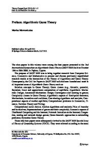


![[Read] Algorithmic Game Theory PDF Best Collection By - Google Sites](https://m.moam.info/img/260x300/read-algorithmic-game-theory-pdf-best-collection-b_647715db097c474b228ba990.jpg)
![[PDF] Algorithmic Game Theory Popular Books - Google Sites](https://m.moam.info/img/260x300/pdf-algorithmic-game-theory-popular-books-google-s_647715dc097c4796708b4bfc.jpg)


![[PDF BOOK] Algorithmic Game Theory EPUB By - Google Sites](https://m.moam.info/img/260x300/pdf-book-algorithmic-game-theory-epub-by-google-si_6477d146097c474c228c7290.jpg)


