sultant and determines ways that the structure can be flexible. 1 Introduction. This project results from the recent convergence of four topics: systems of polyno-.
Algorithmic Search for Flexibility Using Resultants of Polynomial Systems Robert H. Lewis1 and Evangelos A. Coutsias2 1
2
Fordham University, New York, NY 10458, USA University of New Mexico, Albuquerque, NM 87131, USA
Abstract. This paper describes the recent convergence of four topics: polynomial systems, flexibility of three dimensional objects, computational chemistry, and computer algebra. We discuss a way to solve systems of polynomial equations with resultants. Using ideas of Bricard, we find a system of polynomial equations that models a configuration of quadrilaterals that is equivalent to some three dimensional structures. These structures are of interest in computational chemistry, as they represent molecules. We then describe an algorithm that examines the resultant and determines ways that the structure can be flexible.
1
Introduction
This project results from the recent convergence of four topics: systems of polynomial equations, flexibility of three dimensional objects, computational chemistry, and computer algebra. Protein folding has been a major research topic in computational chemistry for a number of years [9]. Proteins are long molecular chains. Proteins form as flexible chains but they quickly fold into shapes that are rigidified by the formation of additional bonds. However, they retain flexibility in certain regions, which is essential for performing their various functions [25]. As macromolecules, composed of relatively heavy atoms (Carbon, Oxygen, Nitrogen, etc.) their conformational problem is modeled in terms of frameworks, i.e., systems of ideal points (atoms) connected by rigid rods (molecular bonds), with fixed angles (the bond angles, determined by molecular orbitals) but flexible torsions (the solid angles formed by successive bonded quartets) [13]. Simple examples are easily built using plastic balls and sticks. In 1812, Cauchy considered flexibility of three dimensional polyhedra (think of a geodesic dome) where each joint can pivot or hinge. He proved that a convex polyhedron with invariant facets must be rigid [4]. Bricard [2], in response to a question posed in 1895 by C. Stephanos [24], gave the geometric conditions under which an octahedron may be flexible. The Bricard octahedra, however, besides being non-convex are also non-embeddable in 3-dimensional space as they possess intercrossing facets. A genuine, embeddable, flexible polyhedron with rigid facets was found by Connelly in 1978 [5], and soon models appeared of a simple flexible structure [8]. It is very enlightening to hold one of these and feel it move. F. Botana and T. Recio (Eds.): ADG 2006, LNAI 4869, pp. 68–79, 2007. c Springer-Verlag Berlin Heidelberg 2007 �
Algorithmic Search for Flexibility Using Resultants of Polynomial Systems
69
As the facets are triangular, they are rigid – unlike quadrilaterals which are inherently flexible; think for example of a cube as compared to a tetrahedron. Thus the deformability is seen in terms of changes of the dihedrals formed by these facets about the edges of the polyhedron. Since the underlying description is in terms of quadratic distance constraints, expressing the conformational problem of the polyhedron in terms of cosines and sines (or half-tangents) of these dihedral angles results in systems of polynomial equations, quadratic in each of these variables, and in which the edge lengths enter as parameters. A polyhedron composed of triangular facets is subject to enough such constraints that according to classical results on rigidity that date back to Lagrange [12] and Maxwell [19] it should be rigid – generically at least! The polynomial system describing these conformations must therefore generically possess a discrete solution set. However, when conditions for flexibility are met, the solution set must acquire components of nonzero dimensionality (so called continuous components). Thus, the problem of detecting flexibility amounts to being able to identify conditions in the parameters for which a system of n polynomials in n variables drops in rank [23]. Here we present a new approach to understanding flexibility, using resultants and symbolic computation. The geometry of the object or molecule is described by a set of multivariate polynomial equations. Solving a system of multivariate polynomial equations is a classic, difficult problem. The approach via resultants was pioneered by Bezout [1], Dixon [10], and others. The resultant res appears as a factor of the determinant det of a matrix containing multivariate polynomials. But often det is too large to compute or factor, even though res is relatively small. We will describe a heuristic that overcomes the problem here, and in other cases [16]. Once we have the resultant, we describe an algorithm that examines the resultant and determines ways that the structure can be flexible. We discover in this way the conditions of flexibility for an arrangement of quadrilaterals in [2]. This system was posed by Bricard as an easily realizable, mathematically equivalent alternative to his flexible octahedra. All computations below were done with Lewis’s computer algebra system Fermat [14], which excels as polynomial and matrix computations [20]. We used a 1.8 ghz Macintosh G5, with 2 gigabytes of RAM, new in 2003.
2
Accelerating the Dixon Resultant
The Dixon Resultant method [10], following an idea of Bezout [1] and modified by Kapur et. al. [11], is presented in [11], [3], and [17]. Given a system of n polynomial equations fi (x1 , x2 , x3 , . . . , a, b, . . .) = 0, i = 1, . . . , n in n − 1 variables xi and a number of parameters a, b, . . ., the method computes its resultant, i.e. a single polynomial in the parameters encapsulating the solution (common zero) to the system. A common variation is to have n equations in n
70
R.H. Lewis and E.A. Coutsias
variables. Then one of them, say x1 , is considered a parameter to bring this into the previous form. In either case, the other variables have been eliminated. In this paper all polynomials have coefficients in the ring of integers Z and the solutions are in the field C of complex numbers. All computations are exact. The basic Bezout-Dixon idea is to construct a square matrix M whose determinant det �= 0 is a multiple of the resultant. The factors of det that are not the resultant are called the spurious factors, and their product is sometimes called the spurious factor. The naive way to proceed is to compute det, factor it, and separate the spurious factor from the actual resultant. Deciding what is spurious and what is the resultant is not always simple. However, when the original problem is based on geometry (as is the present problem) and one knows that the solution set is discrete, the resultant must involve all the parameters. (Otherwise, one parameter could have arbitrary values without affecting the variables. This will not occur in any realistic problem.) Typically, many factors of det do not involve all the parameters. Also, it is usually easy to simply plug in a known numerical solution and see which factor it satisfies. (The Dixon method is not guaranteed to work if the solution set is infinite; see [3]). A graver problem is that the determinant may be so large as to be impractical or even impossible to compute, even though the resultant is relatively small; the spurious factor is huge. Further, the determinant may be so large that factoring it is impractical. To overcome these problems, Lewis has developed several heuristic methods [16]. A method called EDF, Early Discovery of Factors, makes use of the existence of spurious factors. We reproduce it here for the convenience of the reader. By elementary row and column manipulations (Gaussian elimination), it discovers probable factors of det and plucks them out of M0 ≡ M . Any denominators that form in the matrix are plucked out. This produces a smaller matrix M1 still with polynomial entries, and a list of discovered numerators and denominators. Iterate. Here is a summary: Algorithm EDF: Variation of Gaussian elimination to discover factors of the determinant. Input: square matrix M . Let n = number of rows of M . All entries of M are polynomials. Assume Det(M ) �= 0. Output: list of polynomials whose product is Det(M ). Let num be a list of numerator polynomials, initially empty. Let den be a list of denominator polynomials, initially empty. Let M[i] be the submatrix of M from entry (i,i) down to (n,n). for i = 1 to n do for j = i to n do Find the GCD of all entries in row j. Factor it out; append it to num. Find the GCD of all entries in column j.
Algorithmic Search for Flexibility Using Resultants of Polynomial Systems
71
Factor it out; append it to num. endfor; Find a good pivot in M[i]. Move it into position (i,i). Do one step of Gaussian elimination using the pivot. for j = i to n do Find the LCM of all denominators in row j. Multiply it by row j; append it to den. endfor; if desired(i) { every fifth or tenth row is reasonable. } Look for common factors in num and den lists. Consolidate num, den by dividing out such factors. endif endfor. Consolidate num and den lists. den should be empty. Output num. Notes: – The resultant is usually in the numerator list. It is often the last entry. The remaining entries in the numerator list are then the spurious factors. Almost always the numerator list is long and interesting. – If the determinant is irreducible, the final list of numerators must be trivial, i.e., just that one polynomial. But if it is not irreducible, there is no guarantee that the final list of numerators will be nontrivial. – The “consolidate” step, in which we look for a common gcd among the numerator and denominator lists, can be scheduled in various ways, and this can have a noticeable affect on performance. There is no obviously best method. Experiments show that consolidation should be done every five to ten rows. – The definition of “good pivot” is also not rigorous. Basically, one wants the “smallest” nonzero entry, so that the ensuing rational function arithmetic yields “small” entries in the rest of the matrix. Heuristics can be written depending on the number of terms, number of variables, their degree, and the size of the numerical coefficients. EDF can work efficiently because det usually has many factors. This is a bad way to compute the determinant of a random matrix. But the Dixon matrices M are far from random. The total CPU time with this method is not always less than that of a standard determinant method; sometimes it is much more. We will see below that this technique can be dramatically successful. For other examples, see [16].
3
Flexibility of Polyhedra, and Computational Chemistry
This is a very old question. In two dimensions we may consider triangles, quadrilaterals, parallelograms, or more general n-gons. We imagine they are made of
72
R.H. Lewis and E.A. Coutsias
rigid rods connected by pins that are free to pivot at ideal joints. Triangles are obviously rigid, and any quadrilateral is flexible, though parallelograms are more flexible in that the angle at any two sides can take on any value. In three dimensions we likewise consider elementary chemical models, or polyhedra with triangular faces (like a geodesic dome). In 1812 Cauchy [4] proved that convex polyhedra must be rigid. In 1897 Bricard [2] investigated nonconvex octahedra and found three ways they could be flexible. However, his examples are not embeddable in 3-space; they are selfintersecting. So the question was left unanswered, do there exist flexible polyhedra in 3-space? Surprisingly, in 1978 Robert Connelly [5] gave an example, with 18 triangular faces. Steffen [18] found a flexible polyhedron with only 14 triangular faces and 9 vertices. Maksimov [18] proved that Steffen’s is the simplest possible flexible polyhedron composed of only triangles. See also [22]. It was later proved by Sabitov [21] that the volume of any such flexible polyhedron is invariant as it flexes. Coutsias et. al. [6] [7] showed that Bricard’s ideas have application to computational chemistry, and generalized them to solve the problem of Loop Closure, leading to a general algorithm for computing localized torsional deformations of molecular loops in proteins and nucleic acids. Bricard [2] states that the conformational problem of the octahedron is mathematically analogous to that of a system of articulated quadrilaterals. Such systems were important in the late 19th century, with applications to the transfer of force or motion in mechanical devices like sewing machines and automobiles, and today to robotic manipulators. While generically flexible systems where the number of variables exceeds the number of constraints are ubiquitous, here we are concerned with non-generic flexibility, where the number of variables and constraints are equal. Then flexibility is encountered only when certain conditions hold among the parameters of the system. In particular, we shall consider the flexibility of the planar group of three quadrilaterals in figure 1. Corners A, B, C, D, F are freely hinged. AD, DC, CB, BA, GF, FE, HI are rigid rods. The joints at G, H, I, and E can pivot.
4
Algorithmic Approach
We want to write a program that will determine conditions for the geometric figure to be flexible. Our method: – Label the sides e, b, s1 , . . . , s9 (see figure 1). – With elementary analytic geometry find six equations relating the sides to the three angles alpha, beta, gamma at the base. – Eliminate most of the variables; compute the resultant. – Find a way to tell from the resultant when the figure is flexible. 4.1
The Equations
Finding the equations is elementary. The variables are ca, sa, cb, sb, cg, sg (sines and cosines of base angles). There are eleven parameters, e, b, s1 , . . . , s9 .
Algorithmic Search for Flexibility Using Resultants of Polynomial Systems
73
Fig. 1. Configuration of three quadrilaterals from Bricard [2]
Expressions for each x and y coordinate for each point C, G, H, . . . are easily found: cx := b + e + s9 ∗ cg; cy := s9 ∗ sg; gx := s7 ∗ ca; gy := s7 ∗ sa; hx := e + s8 ∗ cb; hy := s8 ∗ sb; .... To form the six equations set each of these to 0 (the last three are just distances in the plane): sa2 + ca2 − 1, sg 2 + cg 2 − 1, sb2 + cb2 − 1, (dx − cx)2 + (dy − cy)2 − s24 , (ix − hx)2 + (iy − hy)2 − s26 , (f x − gx)2 + (f y − gy)2 − s25 We have six equations, six variables, eleven parameters. The latter three equations are actually quite messy because the expressions cx, cy, hx, hy, . . . must be expanded in terms of the variables and parameters. 4.2
Solving the System with the EDF Method
We now apply the Dixon resultant method to the six equations, eliminating all variables but ca. The resultant will be a function of ca and the eleven parameters. The Dixon matrix M is 29 × 29. The EDF method described in section 2 takes 62 minutes on the desktop Macintosh computer, and yields a list of numerators with more than 80 entries. The last two have 275808 and 312783 terms. Dividing each by their easily found contents c1 , c2 , yields the same polynomial of 201694
74
R.H. Lewis and E.A. Coutsias
terms (recall that the content of a polynomial f (x, . . .) relative to x is the gcd of all the coefficients of xk , k = 0, . . . , degree(f, x)). This polynomial, call it res, is easily checked to be irreducible and is the resultant. It has degree 7 in ca. The product of the other terms in the list, call it h, has 35000 terms. The determinant of M , as the product of all these, res2 h c1 c2 , is truly gigantic, probably not computable on any computer. Thanks to EDF, there is no need to compute it. 4.3
Determining Flexibility
Classically, one would use the resultant by plugging in numerical values for the eleven parameters. That yields an equation in only the one variable ca that could be solved numerically. But how to detect flexibility in the quadrilaterals? Answer: If the parameters have the right relations to each other to produce flexibility, there are infinitely many values that work for ca. But res is a polynomial, so the only way to have that many roots is for every coefficient relative to ca in the resultant to vanish. That can be thought of as yielding eight new equations in the eleven sides, but those equations would be too complicated to use (their number of terms ranges from 198 to over 53000), Instead, we have developed an algorithm Solve to produce a list of relations among the sides that will kill all eight coefficients. If the algorithm is good enough, any relationship producing flexibility will be on this list. However, it is not clear that all relationships on the list must produce flexibility. The issue of converse implication with the Dixon resultant is discussed in [3]. If a set of relations force all eight coefficients of res to vanish, when these relations are plugged into the original six equations, there is a positive-dimensional component to the solution set (i.e., a continuous family of solutions). But this may not be meaningful geometrically. To describe the algorithm, let us first rename e ≡ s10 , b ≡ s11 . We present Solve in terms of general inputs f and x. f is a polynomial in x and N parameters si . Algorithm Solve(f, x): Given a polynomial f in a variable x and a number N of parameters si , find relations on the parameters that make the entire polynomial vanish. Our problem is solved by invoking Solve(res, ca), N = 11. Outline: 1. Kill each coefficient coef of x in turn, starting at the highest degree. Do so by looking for contents, linear parameters to solve for, or a difference of squares. When a substitution is found (it is possible that none will be found), plug it in, reducing the degree of f . Continue. 2. Whether or not substitutions were found in Step 1, also try to kill the coefficient coef by invoking the entire algorithm on it, relative to each variable in coef. So, this step of Solve works by calling Solve(coef, si ) within a loop. 3. Use suitable data structures to keep track of all the substitutions.
Algorithmic Search for Flexibility Using Resultants of Polynomial Systems
75
Here is a simple example. If res were (s9 ∗s8 −s7 ∗s6 )ca2 +(s4 2 −s3 2 )ca+s8 −s6 , one solution would be the collection (or table) of the three relations s9 = s7 , s8 = s6 , s4 = s3 . On the other hand, the algorithm will fail on something random like (5s6 3 s9 6 + 2s9 4 − 7s34 s6 4 s9 + 1)ca2 + (3s5 4 s6 3 s9 7 + 2s7 4 + 7)ca + s5 4 + s6 3 s9 5 − s5 3 s6 4 s9 + 2 as none of the techniques in Step 1 apply to the coefficients of ca. The relations may be described as follows: Partition the set of N parameters into nonempty subsets X = {xi }ni=1 , Y = {yj }m j=1 , n + m = N . Each relation is an equation yj = gj (xi1 , xi2 , . . .) where gj is a rational function. A collection of m of these for j = 1, . . . , m is a solution table if f evaluated at them all is 0. In the example above X = {s3 , s6 , s7 } and Y = {s4 , s8 , s9 }. Input: multivariate polynomial f in a primary variable x and N parameters si . Output: list of solution tables, as defined above. Let lst be the output list of solution tables, initially empty. Let cc = leading coefficient in f(x). { cc is a polynomial in the parameters. } Get factors of cc by finding content relative to all s_i. { Optionally, also do more complete factoring. } Use the factors to produce a list ls of s_j to solve for: Within each factor, find all s_j of degree 1. Look for factors that are differences of squares. { Note: the list ls may be empty. } while not done with the list ls do Solve for s_j, getting s_j = g(s_i_1, s_i_2, ...). Use the relation g to replace s_j in f. This yields fj(x), say, of lower degree. Compute lstj = Solve(fj,x). if lstj is not empty Insert the relation s_j = g into each table of lstj. Append the resulting lstj to lst. endif; enddo; for every s_i in cc not in ls do Compute lsti = Solve(cc, s_i). for every table T in lsti do plug the relations of T into f, yielding ft(x). Compute lstt = Solve(ft, x). Combine T with each table in lstt. Append the resulting lstt to lst. endfor; endfor; Look for duplicates in lst; "clean up" lst. Output lst.
76
R.H. Lewis and E.A. Coutsias
In creating the relations sj = g(si1 , si2 , . . .), we reject any relation of the form sj = 0, or in which all the numerical coefficients in g are negative, such as s3 = −s2 − s5 s7 . Since the si are lengths on a geometric figure, these are meaningless. Details of combining and managing the table lists are left to the programmer. Documented Fermat code for this algorithm is at [15]. There is no guarantee this method will work. However it does, in about 3 minutes. Thirteen tables are produced, all of which are variations or special cases of the following three. It finds the two ways to make the quadrilaterals flexible: all three are parallelograms, and one is a parallelogram and the other two are similar. Interestingly, it also finds a degenerate yet still meaningful arrangement when two of them are rhomboids. For example, the case where the lower left quadrilateral is a parallelogram and the other two are similar is expressed by the table s9 s8 s7 s6 s5
= s3 (e + b)/b, = s1 b/(e + b), = s2 , = s4 b/(e + b), =e
All three parallelograms is s9 s4 s7 s5 s6 s8
= s1 , = e + b, = s2 , =e = b, = s3
Two rhomboids is s9 s8 s4 s3
= e + b, = s6 , = s1 , =b
Let us look more closely at the two rhomboids case. If those relations are substituted into the original six equations, one equation becomes extremely simple: (b − s6 cb)(1 + cg) − s6 sg sb. We are led to setting cg = −1 and sg = 0 (so γ = π), which kills three (not just two) of the six equations. Three remain, in the four variables sa, ca, sb, cb: sa2 + ca2 − 1, sb2 + cb2 − 1, 2 s2 s7 sb sa + 2 s2 s7 ca cb − 2 e s2 cb + 2 e s7 ca − s7 2 + s5 2 − s2 2 − e2
Algorithmic Search for Flexibility Using Resultants of Polynomial Systems
77
We expect therefore a continuous family of solutions, which can be demonstrated by numerical experiments, or by computing the (bi-variate) resultant of the three equations, eliminating sa and sb: 8 e s2 2 s7 ca cb2 − 4 s2 2 s7 2 cb2 − 4 e2 s2 2 cb2 − 8 e s2 s7 2 ca2 cb + 4 s2 s7 3 ca cb − 4 s2 s5 2 s7 cacb + 4 s2 3 s7 cacb + 12 e2s2 s7 cacb − 4 e s2 s7 2 cb + 4 e s2 s5 2 cb − 4 e s2 3 cb − 4 e3 s2 cb−4 s22 s7 2 ca2 −4 e2 s7 2 ca2 +4 e s73 ca−4 e s52 s7 ca+4 e s22 s7 ca+4 e3 s7 ca− s7 4 + 2 s5 2 s7 2 + 2 s2 2 s7 2 − 2 e 2 s7 2 − s5 4 + 2 s2 2 s5 2 + 2 e 2 s5 2 − s2 4 − 2 e 2 s2 2 − e 4 . The choice cg = −1, sg = 0 is actually geometrically meaningful. It corresponds to two degenerate rhomboids, with the points A, C and E, I falling on top of each other. Thus, the flexibility in this case is just the flexibility of the single quadrilateral AEF G. The original six equations do indeed fit this picture. See figure 2. If, on the other hand, we exclude the degeneracy of the angle γ, then it can be shown that the resulting problem has a resultant of lower degree, leading to additional, non-degenerate, discrete conformations. The identical vanishing of the resultant of the full problem for this case would completely mask the existence of these discrete components of the solution set.
Fig. 2. Degenerate rhomboids
4.4
Future Work
By writing the equations in terms of the tangents of the half-angles, we can reduce the problem from six to three equations: a1 ∗ t21 ∗ t22 + b1 ∗ t21 + 2c1 ∗ t1 ∗ t2 + d1 ∗ t22 + e1 = 0, a2 ∗ t22 ∗ t23 + b2 ∗ t22 + 2c2 ∗ t2 ∗ t3 + d2 ∗ t23 + e2 = 0, a3 ∗ t21 ∗ t23 + b3 ∗ t21 + 2c3 ∗ t1 ∗ t3 + d3 ∗ t23 + e3 = 0 The ti are the half-angle tangents of the three base angles. As before, these equations result from elementary analytic geometry. The parameters ai , bi , . . . are quadratic functions of the eleven sides. For example, a1 = e2 + s22 + s27 − s25 − 2e ∗ s2 + 2e ∗ s7 − 2s2 ∗ s7
78
R.H. Lewis and E.A. Coutsias
which is a product of two linear terms. This is the form of the equations as derived by Bricard. The resultant of this system has 5685 terms. Shall we apply our flexibility searching algorithm as before? It is more subtle, as now we must try relations like a1 = 0 or a1 = −d3 − e2 . When the parameters were actually the sides, substitutions like this made no sense and were excluded, thereby streamlining the search. We have recently modified algorithm Solve to consider these cases, and the work is ongoing. Success on this set of three equations would be significant because the identical set of equations arises in other contexts, and a variant (including also the “missing” terms, such as t21 t2 , t3 , . . .) gives the conformational equations of a protein or nucleic acid backbone [6], [7].
References 1. Bikker, P.: On Bezout’s method for computing the resultant. RISC-Linz Report Series, Johannes Kepler University A-4040 Linz, Austria (1995) 2. Bricard, R.: M´emoire sur la th´eorie de l’octa`edre articul´e. J. Math. Pures Appl. 3, 113–150 (1897), English translation: http://www.math.unm.edu/∼ {}vageli/papers/bricard.pdf 3. Buse, L., Elkadi, M., Mourrain, B.: Generalized resultants over unirational algebraic varieties. J. Symbolic Comp. 29, 515–526 (2000) ´ 4. Cauchy, A.-L.: Deuxi`eme m´emoire sur les polygones et les poly`edres. J. de l’Ecole Polyt. 16(1813), 87–99 5. Connelly, R.: A counterexample to the rigidity conjecture for polyhedra. Publ. Math. I. H. E. S. 47, 333–338 (1978) 6. Coutsias, E.A., Seok, C., Wester, M.J., Dill, K.A.: Resultants and loop closure. International Journal of Quantum Chemistry 106(1), 176–189 (2005) 7. Coutsias, E.A., Seok, C., Jacobson, M.J., Dill, K.A.: A Kinematic view of loop closure. Journal of Computational Chemistry 25(4), 510–528 (2004) 8. Cromwell, P.R.: Polyhedra, pp. 222–224. Cambridge University Press, New York (1997) 9. Dill, K. A.,, Chan, H.S.: From Levinthal to pathways to funnels: The “new view” of protein folding kinetics. Nat. Struct. Biol. 4, 10–19 (1997) 10. Dixon, A.L.: The eliminant of three quantics in two independent variables. Proc. London Math. Society 6, 468–478 (1908) 11. Kapur, D., Saxena, T., Yang, L.: Algebraic and geometric reasoning using Dixon resultants. In: Proc. of the International Symposium on Symbolic and Algebraic Computation., A.C.M. Press, New York (1994) 12. Lagrange, J.-L.: M´ecanique Analytique, Paris (1788) 13. Leach, A.: Molecular Modeling and Simulation, Cambridge (2004) 14. Lewis, R.H.: Computer algebra system Fermat. http://home.bway.net/lewis/ 15. Lewis, R.H.: Fermat code for Solve. http://home.bway.net/lewis/ 16. Lewis, R.H.: Heuristics to accelerate the Dixon resultant. to appear in Mathematics and Computers in Simulation 17. Lewis, R.,, Stiller, P.: Solving the recognition problem for six lines using the Dixon resultant. Mathematics and Computers in Simulation 49, 203–219 (1999) 18. Maksimov, I.G.: Polyhedra with bendings and Riemann surfaces. Uspekhi Matemat. Nauk 50, 821–823 (1995)
Algorithmic Search for Flexibility Using Resultants of Polynomial Systems
79
19. Maxwell, J.C.: On the calculation of equilibrium and stiffness of frames. Phil. Mag. 27, 294–299 (1864) 20. Robertz, D., Gerdt, V.: Comparison of software systems (2004), http://home.bway.net/lewis/ 21. Sabitov, I.: A proof of the “bellows” conjecture for polyhedra of low topological genus. Dokl. Acad. Nauk 358(6), 743–746 (1998) 22. Stachel, H.: Higher order flexibility of octahedra. Period. Math. Hung. 39, 225–240 (1999) 23. Sommese, A.J., Wampler II, C.W.: The Numerical Solution of Systems of Polynomial arising in Engineering and Science. World Scientific, New York (2005) 24. Stephanos, Cyparissos.: Problem 376. L’ Interm´ediaire des Math´ematiciens, 2, 243–244 (1895) 25. Thorpe, M., Lei, M., Rader, A.J., Jacobs, D.J., Kuhn, L.: Protein flexibility and dynamics using constraint theory. Journal of Molecular Graphics and Modelling 19, 60–69 (2001)