1.
Algorithms for Asynchronous Track-to-Track Fusion XIN TIAN YAAKOV BAR-SHALOM
Most track-to-track fusion (T2TF) algorithms for distributed tracking systems in the literature assume that the local trackers are synchronized. However, in the real world, synchronization cannot be usually achieved among distributed local trackers where local measurements are obtained and local tracks are updated at different times with different rates. In addition, communication links between local trackers and the fusion center (FC) are subject to possible delays, which results in delayed local tracks for the fusion at the FC. This paper presents and compares algorithms for asynchronous Track-to-Track Fusion (AT2TF) for the fusion of asynchronous and delayed tracks. First, the optimal algorithm for AT2TF with no memory and with partial information feedback (AT2TFwoMpf) is presented. The algorithm, denoted as AT2TFwoMpfOpt, serves as the baseline algorithm for performance comparison. Three approximate AT2TF algorithms from the literature are compared with AT2TFwoMpfOpt and are shown to have consistency problems and loss in fusion accuracy. Then the Information Matrix Fusion (IMF) algorithm from the literature is generalized for the fusion of asynchronous tracks. Based on the generalized IMF (GIMF), AT2TF algorithms are derived for the information configurations with both partial and full information feedback. These algorithms are shown to have good consistency and nearly optimal fusion accuracy. Due to the simplicity of their implementation, these algorithms are appealing candidates for practical applications.
Manuscript received January 1, 2010; released for publication July 7, 2010. Refereeing of this contribution was handled by Stefano Coraluppi. Authors’ address: Dept. of Electrical and Computer Engineering, University of Connecticut, Storrs CT 06269-2157, E-mail: fxin.tian,
[email protected].
c 2010 JAIF 1557-6418/10/$17.00 ° 128
INTRODUCTION
Algorithms for synchronous track-to-track fusion (T2TF) have been widely studied. For the optimal T2TF, it is critical to take into account the crosscovariances between tracks of the same target due to (i) the common process noise, and (ii) information feedback [2]. The optimal memoryless (without memory–“woM”) T2TF with no information feedback (T2TFwoMnf) was studied in [3], [11]. In [15], the complete set of information configurations and the optimal algorithms for the synchronous T2TF were presented. These are T2TF without memory (T2TFwoM) with no, partial and full information feedback (designated as T2TFwoMnf, T2TFwoMpf and T2TFwoMff, respectively), as well as T2TF with memory (T2TFwM) with no, partial and full information feedback (designated as T2TFwMnf, T2TFwMpf and T2TFwff). The information matrix fusion (IMF) [14, 8] is a special case of T2TFwM. The advantage of IMF over the optimal T2TF is that it does not require the crosscovariances between the local tracks, which greatly simplifies its implementation. However, IMF is optimal only when the fuser operates at full rate [8, 7]. For reduced rate, IMF is heuristic. As reported in [6], IMF has consistency problems for extremely large process noise levels; however for most tracking scenarios it is consistent and has good tracking accuracy. In the real world, synchronization cannot be usually achieved among distributed local trackers where local measurements are obtained and local tracks are updated at different time instants. In addition, the communication between local trackers and the fusion center (FC) is subject to possible delays, and thus the fusion of delayed tracks should also be addressed. In [5] the problem of the fusion of delayed tracks is converted and solved as the fusion of out-of-sequence measurements (OOSM). However, the algorithm deals only with the fusion of delayed synchronous tracks at full rate. A pseudo measurement approach of fusing asynchronous tracks can be found in [12]. In [13], three approximate algorithms for AT2TF were proposed. Later in the present research, they are evaluated by simulations and shown to have consistency problems. This is because the crosscorrelation between the central and local tracks due to information feedback is not accounted. In this paper, first, the optimal (under linear Gaussian–LG–assumption) synchronous T2TF algorithm is generalized for the asynchronous situation, where the information configuration of memoryless fusion with partial information feedback (feedback only to the central track) [15] is used. The resulting algorithm accounts exactly for the crosscovariances between the central and local tracks. It handles both the asynchronous sampling times of the local trackers and the fusion of delayed tracks, and guarantees the consistency of the fused estimates. The optimal algorithms for the more complicated AT2TF with memory is not considered here, due to the limited gain in tracking accuracy, especially when significant geometric diversity exists among the local
JOURNAL OF ADVANCES IN INFORMATION FUSION
VOL. 5, NO. 2
DECEMBER 2010
tracks.1 The drawback of the optimal AT2TF algorithm is its high communication cost and high complexity, which is very difficult to use for scenarios with more than two trackers and AT2TF with full information feedback. Then the Information Matrix Fusion (IMF) is generalized for the fusion of asynchronous tracks. The algorithm for AT2TF with partial information feedback (AT2TFpf) based on the generalized IMF (GIMF) approach, denoted as AT2TFpfIMF, is presented and compared with AT2TFwoMpfOpt. It is shown that AT2TFpfIMF, although heuristic, is consistent and has a similar level of fusion accuracy as AT2TFwoMpfOpt. Due to the simplicity of AT2TFpfIMF compared to AT2TFwoMpfOpt, it is an appealing candidate for practical applications. Finally, the use of the GIMF approach for AT2TF with full information feedback (AT2TFff) is presented. The resulting fusion algorithm AT2TFffIMF is shown to yield consistent and accurate fusion results. Its variations with further savings in communication and little loss in fusion consistency and accuracy are also investigated. The paper is organized as follows. Section 2 formulates the AT2TF problem. Section 3 presents the optimal fusion algorithm, AT2TFwoMpfOpt. Section 4 compares AT2TFwoMpfOpt with three approximate algorithms from [13]. Section 5 presents and evaluates the GIMF based algorithms for AT2TF with partial and full information feedback. The paper is summarized in Section 6.
after the fusion, track 1 continues with the fused track (xˆ c (k j k), Pc (k j k)) which has improved accuracy, while local tracker 2 operates by itself unaffected by the fusion. For AT2TF with full information feedback, the fused track is sent back to tracker 2. When the feedback arrives, tracker 2 will fuse it with its local information and continue with the fused result. (See Section 5.3 for the details.) 3.
THE OPTIMAL ALGORITHM FOR AT2TFPF WITHOUT MEMORY AND WITH PARTIAL INFORMATION FEEDBACK–AT2TFWOMPFOPT
The optimal algorithm for asynchronous T2TF (AT2TF) is presented only for the configuration of fusion with no memory and with partial information feedback, in view of the following facts: ² T2TF with no memory has some performance loss compared to the T2TF with memory; however, this is not significant especially when there is significant geometric diversity among the local trackers. ² For AT2TF in the presence of communication delays, the exact algorithm for the configuration with full information feedback is impractical.
(1) where (xˆ c (tf j tf ), Pc (tf j tf )) is the fused track. Depending on the fusion algorithm, additional information will be required, which is indicated by the “: : : ” in (1). For the configuration with partial information feedback,
The objective of the AT2TF is to fused track 1, given by xˆ 1 (tf j tf ), P1 (tf j tf ), with the predicted track 2, given by xˆ 2 (tf j tc ), P2 (tf j tc ). Compared to the synchronous T2TF [15], there are two additional issues to address. The first one is that the sampling (measurement) times of the two trackers are different. This causes difficulties for the calculation of the crosscovariances between tracks. The solution to this problem is to use the union of the sampling times, where zero filter gains are used for the tracks at sampling times when there is no actual measurement available for update. Then the crosscovariance between tracks can be calculated as in the synchronized case using (2) below. Fig. 1 illustrates the idea of the union of the sampling times. Fig. 1(a) shows the time axis of tracker 1, on which the black circles indicate when tracker 1 received measurements and did actual track updates.3 Fig. 1(b) shows the same for track 2. Fig. 1(c) shows the union of the sampling times of the two trackers on the same time axis. Then tracks 1 and 2 are discretized according to the union of the sampling times in Fig. 1(d)—(e), where the black circles represent actual track updates and the white circles represent virtual track updates, i.e., with zero filter gains. To differentiate the original tracks and the discretized tracks according to the union of the sampling times, the latter are denoted as xˆ i¤ with “*” superscript for the track index. The exact crosscovariance between the two tracks at the any time ta > tl is calculated as
1 In such cases, track estimates from the local trackers provide complementary perspectives of the target state. 2 The problem of track-to-track association is not considered.
3 It is assumed that the local trackers have no delay between when a measurement is taken and the track update. Delay is assumed in the communication between tracker 2 and the FC.
2. PROBLEM FORMULATION For the sake of simplicity, the basic scenario of the fusion of two tracks of a target from two local trackers is considered.2 The trackers operate asynchronously with sampling intervals T1 and T2 . Tracker 1 is collocated with the FC, whose track is available for fusion with no time delay. Tracker 2 is a remote tracker which sends its track (xˆ 2 (tc j tc ), P2 (tc j tc )) to the FC once in a while, where the communication time tc is the time stamp of the local track. The track arrives at the FC with a random communication delay TD . When track 2 is received, the FC fuses track 1 with the delayed track 2 at fusion time tf (with tf ¸ tc + TD ), which can be written as [xˆ c (tf j tf ), Pc (tf j tf )] = f[xˆ 1 (tf j tf ), P1 (tf j tf ), xˆ 2 (tc j tc ), P2 (tc j tc ), : : :]
ALGORITHMS FOR ASYNCHRONOUS TRACK-TO-TRACK FUSION
129
crosscovariance between the local tracks. The flowchart in Fig. 2 for the crosscovariance calculation and trackto-track fusion should be carefully followed. Starting from the first fusion, as shown in Fig. 2(a), tl(1) denotes the prior time of the 1st fusion when the most upto-date covariances and crosscovariances between the two tracks, i.e., P1 (tl(1) j tl(1) ), P2 (tl(1) j tl(1) ) and P12 (tl(1) j tl(1) ), are available at the FC. The communication time tc(1) is the time when track 2, namely, (xˆ 2 (tc(1) j tc(1) ), P2 (tc(1) j tc(1) )), is sent to the FC for the first fusion. Due to the time delay in data transmission, at fusion time tf(1) , track (xˆ 1 (tf(1) j tf(1) ), P1 (tf(1) j tf(1) )) will be fused with the predicted track (xˆ 2 (tf(1) j tc(1) ), P2 (tf(1) j tc(1) )). The first fusion is done as follows ² Discretize both track 1 and the delayed track 2 from tl(1) to tf(1) according to the union of the sampling times. ² Propagate the prior information from tl(1) to tc(1)
Fig. 1. The union of the sampling times.
follows P1¤ 2¤ (ta j ta ) = W1e¤ (ta , tl )P1¤ 2¤ (tl j tl )W2e¤ (ta , tl )0 +
a X
W1v¤ (ta , ti¡1 )Q(ti , ti¡1 )W2v¤ (ta , ti¡1 )0
i=l+1
(2) where tl , designated as the “prior time,” is the most recent time at which the crosscovariance between the two tracks is available; the summation in (2) is over the set ftl , : : : , ta g, which is the union of the sampling times in the time interval [tl , ta ]; and Y
a¡l¡1
Wse¤ (ta , tl ) =
i=0
Wsv¤ (ta , ti¡1 )
=¡
[I ¡ Ks¤ (ta¡i) Hs¤ (ta¡i )]F(ta¡i , ta¡i¡1 )
(a¡i¡1 Y j=0
[I ¡ Ks¤ (ta¡j )Hs¤ (ta¡j )]F(ta¡j , ta¡j¡1 )
¢ [I ¡ Ks¤ (ti )Hs¤ (ti )],
s = 1, 2:
(3) ) (4)
where Ks¤ (ti ), i = l + 1, : : : , a are the local Kalman filter gains, which are zero for the virtual updates; Hs¤ (ti ) are the observation matrices at local tracker s and F(ti , ti¡1 ) are the state transition matrices from ti¡1 to ti . Note that the calculation of the exact crosscovariance between two tracks requires the local filter gains and observation matrices at every sampling time, which puts a high requirement on communication capacity. An approximate approach to save communication cost can be found in [15]. Note that, for the synchronous T2TF, the system can use either the Discretized Continuous-time Kinematic Model or the Direct Discrete-Time Kinematic Model (see [1] Secs. 6.2 and 6.3). However, for AT2TF, the use of the union the sampling times requires to break the local process noises down to finer pieces (shorter time intervals). To preserve the process noise whiteness after the finer discretization, only the Discretized Continuous-Time Kinematic Model should be used. The second issue is that the fusion of local estimates with time delays makes it more difficult to calculate the 130
P1¤ (tc(1) j tc(1) ) 8 P (t j t ), if an actual track 1 > > > 1 c(1) c(1) < update occurred at tc(1) = F(tc(1) , tc1 )P1 (tc1 j tc1 )F(tc(1) , tc1 )0 > > > : +Q(tc(1) , tc1 ), otherwise (5) where tc1 is the latest time before tc(1) when track 1 was updated and Q(tc(1) , tc1 ) is the cumulative effect of the process noise in the interval (tc1 , tc(1) ]. For tracker 2 P2¤ (tc(1) j tc(1) ) = P2 (tc(1) j tc(1) )
(6)
and the crosscovariance P1¤ 2¤ (tc(1) j tc(1) ) is calculated using (2) from tl(1) to tc(1) . Note that, with xˆ 2 (tc(1) j tc(1) ) and P2 (tc(1) j tc(1) ) sent to the FC, at this point the covariances and crosscovariances between the two tracks, namely, P1¤ (tc(1) j tc(1) ), P2¤ (tc(1) j tc(1) ) and P1¤ 2¤ (tc(1) j tc(1) ), are available at tc(1) , which makes tc(1) the new prior time tl(2) for the second fusion. ² Then predict the received track 2 from tc(1) to the fusion time tf(1) xˆ 2¤ (tf(1) j tf(1) ) = xˆ 2 (tf(1) j tc(1) ) = F(tf(1) , tc(1) )xˆ 2 (tc(1) j tc(1) )
(7)
P2¤ (tf(1) j tf(1) ) = P2 (tf(1) j tc(1) )
= F(tf(1) , tc(1) )P2 (tc(1) j tc(1) )F(tf(1) , tc(1) )0 + Q(tf(1) , tc(1) )
(8)
where F(tf(1) , tc(1) ) is the state transition matrix from time tc(1) to tf(1) and Q(tf(1) , tc(1) ) is the cumulative effect of the process noises in [tc(1) , tf(1) ].
JOURNAL OF ADVANCES IN INFORMATION FUSION
VOL. 5, NO. 2
DECEMBER 2010
Fig. 2. Flowchart of T2TFwoMpf with feedback to tracker 1 and delayed track 2 (“- - - -” shows prediction).
² With (5)—(6), the crosscovariance P1¤ 2¤ (tf(1) f j tf(1) ) is calculated using the union of the sampling times using (2) from tc(1) to tf(1) . ² xˆ 1¤ (tf(1) j tf(1) ) and P1¤ (tf(1) j tf(1) ) are available at the FC. ² With the information above, the optimal AT2TF is done using the LMMSE fuser [1]
crosscovariance between track 1 and the delayed track from the prior time tl(2) to the new communication time tc(2) , which needs to take into account the impact of the previous fusion. This time (2) can not be used directly, since, after the first fusion, track 1 continued with the fused track (due to the partial information feedback), which contains two parts: one from the old track 1
xˆ c (tf(1) j tf(1) ) = xˆ 1¤ (tf(1) j tf(1) ) + [P1¤ (tf(1) j tf(1) ) ¡ P1¤ 2¤ (tf(1) j tf(1) )] ¢ [P1¤ (tf(1) j tf(1) ) + P2¤ (tf(1) j tf(1) ) ¡ P1¤ 2¤ (tf(1) j tf(1) )0 ¡ P1¤ 1¤ (tf(1) j tf(1) )]¡1 [xˆ 2¤ (tf(1) j tf(1) ) ¡ xˆ 1¤ (tf(1) j tf(1) )] = xˆ 1¤ (tf(1) j tf(1) ) + K1¤ 2¤ (tf(1) )[xˆ 2¤ (tf(1) j tf(1) ) ¡ xˆ 1¤ (tf(1) j tf(1) )] = (I ¡ K1¤ 2¤ (tf(1) ))xˆ 1¤ (tf(1) j tf(1) ) + K1¤ 2¤ (tf(1) )xˆ 2¤ (tf(1) j tf(1) )
(9)
Pc (tf(1) j tf(1) ) = P1¤ (tf(1) j tf(1) ) ¡ [P1¤ (tf(1) j tf(1) ) ¡ P1¤ 2¤ (tf(1) j tf(1) )] ¢ [P1¤ (tf(1) j tf(1) ) + P2¤ (tf(1) j tf(1) ) ¡ P1¤ 2¤ (tf(1) j tf(1) ) ¡ P1¤ 2¤ (tf(1) j tf(1) )0 ]¡1 [P1¤ (tf(1) j tf(1) ) ¡ P1¤ 2¤ (tf(1) j tf(1) )0 ]:
(10) The second fusion, as illustrated in Fig. 2(b),4 is slightly different from the first fusion in propagating the 4 Note
that, in Fig. 2, it is assumed that the second communication happens after the previous fusion. For scenarios where this assumption does not hold, the scheme can be easily modified to accommodate the change.
(indicated by index “o1”), the other from the predicted track 2 (indicated by index “o2”). The crosscovariances P1¤ 2¤ (tc(2) j tc(2) ) in the second fusion is calculated as follows: ² Calculate the crosscovariances Po1¤ 2¤ (tf(1) j tf(1) ) and Po2¤ 2¤ (tf(1) j tf(1) ) using (2) from tc(1) to tf(1) .
ALGORITHMS FOR ASYNCHRONOUS TRACK-TO-TRACK FUSION
131
² Then, by evaluating the crosscovariance between the fused track estimate (9) and local track 2 at tf(1) , one has P1¤ 2¤ (tf(1) j tf(1) ) = (I ¡ K1¤ 2¤ (tf(1) ))Po1¤ 2¤ (tf(1) j tf(1) ) + K1¤ 2¤ (tf(1) )Po2¤ 2¤ (tf(1) j tf(1) ): (11) ² Propagate the crosscovariance P1¤ 2¤ (tf(1) j tf(1) ) from tf(1) to tc(2) using (2). Now, with the new P1¤ 2¤ (tc(2) j tc(2) ) calculated, tc(2) becomes the new prior time for the next fusion, namely tl(3) = tc(2) , and the old prior information can be discarded. The rest of the second fusion can be done exactly the same as in the first fusion. The third fusion and the ones afterwards are done as the second fusion.
Fig. 3. AT2TFwoMpfOpt vs. three approximate AT2TF algorithms: Consistency test (Scenario 1: high process noise).
4. AT2TFWOMPFOPT VS. THREE APPROXIMATE ALGORITHMS FROM THE LITERATURE Three approximate algorithms for AT2TF from [13], denoted as AT2TFpfApprC, AT2TFpfApprB and AT2TFpfApprA, are compared with AT2TFwoMpfOpt proposed in Section 3. AT2TFpfApprC is the simplest one which assumes the errors of the local tracks are independent. AT2TFpfApprB and AT2TFpfApprA consider the crosscovariance between local tracks due to the common process noises. However, neither takes into account the crosscovariance due to the partial information feedback from FC to tracker 1. A 2-D tracking scenario with two local trackers 1 and 2 tracking one target is used. The target motion follows a CWNA model5 in [1] with process noise power spectral density (PSD) q˜ . The target state is de_ 0 , i.e., position and velocity in 2-D fined as x = [» »_ ³ ³] Cartesian coordinates, with initial value set, without loss of generality, as [2000 m, ¡2 m/s, 5000 m, ¡5 m/s]. Tracker 1 is collocated with the FC at the origin (0, 0), while tracker 2 is located at (X2 , Y2 ). Tracker i (i = 1, 2) takes position measurements of the target in its polar coordinates every Ti with zero mean white noise errors. The range standard deviation for both trackers is ¾ir = 10 m and the azimuth standard deviation is ¾ia = 1± . The local tracks are generated using the Converted Measurement Kalman Filter [1]. Tracker 2 sends its track at prespecified time instants to the FC with a communication delay of TD . The simulation results are obtained from 100 Monte Carlo runs. Scenario 1: Fusion of tracks with high process noise intensity and significant geometric diversity. Tracker 2 location: (10000, 0) m; Sampling intervals: T1 = 2 s, T2 = 2:5 s; Process noise PSD: q˜ = 1 m2 =s3 (maneuvering index 0.03—0.3); Comm.; delay: TD = 2 s; Fusion times: [9 : 6 : 147] s. 5 As
explained in Section 3, only the discretized continuous-time kinematic models can be used for AT2TFpfwoMopt.
132
Fig. 4. AT2TFwoMpfOpt vs. three approximate AT2TF algorithms: RMS position errors (Scenario 1: high process noise).
As shown in Figs. 3—4, the optimal fusion algorithm AT2TFwoMpfOpt is consistent by checking the Normalized Estimation Error Squared (NEES), and it has small tracking errors especially at the fusion times. Algorithms AT2TFpfApprA—C, however, have consistency problems, because the crosscorrelation due to the partial information feedback is not accounted for. When the process noise level is high, the impact of this on the RMSE is less significant since the track estimates have short memories. Scenario 2: Fusion of tracks with low process noise intensity and significant geometric diversity. Tracker 2 location: (10000, 0) m; Sampling intervals: T1 = 2 s, T2 = 2:5 s; Low process noise PSD: q˜ = 0:01 m2 =s3 (maneuvering index 0.003—0.03); Comm. delay: TD = 2 s; Fusion times: [9 : 6 : 147] s. As shown in Figs. 5—6, when the process noise level is low, the RMSE performance of the three approximate algorithms becomes worse and their consistency is much worse. COMMENTS ON AT2TFWOMPFOPT ² The optimal algorithm for AT2TF needs to take into account the crosscorrelation between the local tracks due to the common process noise and, especially, the information feedback.
JOURNAL OF ADVANCES IN INFORMATION FUSION
VOL. 5, NO. 2
DECEMBER 2010
Fig. 7. Information flow of AT2TFpfIMF.
Fig. 5. AT2TFwoMpfOpt vs. three approximate AT2TF algorithms: Consistency test (Scenario 2: low process noise).
² track (xˆ 1 (tf j tf ), P 1 (tf j tf )), from tracker 1 (same as FC) ² tracks (xˆ 2 (t1 j t1 ), P 2 (t1 j t1 )) and (xˆ 2 (t2 j t2 ), P 2 (t2 j t2 )) from tracker 2, t1 < t2 · tf . All the above are from the same target. The fused track at tf according to the Generalized Information Matrix fusion (GIMF) is given by P(tf )¡1 = P 1 (tf j tf )¡1 + [P 2 (tf j t2 )¡1 ¡ P 2 (tf j t1 )¡1 ]
(12) P(tf )¡1 xˆ (tf ) = P 1 (tf j tf )¡1 xˆ 1 (tf j tf ) + [P 2 (tf j t2 )¡1 xˆ 2 (tf j t2 ) ¡ P 2 (tf j t1 )¡1 xˆ 2 (tf j t1 )]
(13)
Fig. 6. AT2TFwoMpfOpt vs. three approximate AT2TF algorithms: RMS position errors (Scenario 2: low process noise).
² The drawbacks of the optimal fusion algorithm are its high communication cost and complexity. Approximate algorithms that lower the cost of AT2TFwoMpfOpt can be found in [16]. To avoid the calculation of the crosscovariance, a generalized Information Matrix Fusion (GIMF) [9, 6, 14] can be used for AT2TF. This is discussed in Section 5. 5. THE GENERALIZED INFORMATION MATRIX FUSION FOR AT2TF The Information Matrix Fusion (IMF) [14, 8] is optimal (equivalent to the CMF) only at full rate. At a reduced rate, the algorithm is heuristic, but it works remarkably well over the practical range of process noise levels [7]. In this section, the generalized form of the IMF is presented for asynchronous T2TF. Then, based on the generalized IMF (GIMF), algorithms for AT2TF with partial and full information feedback are presented and evaluated. 5.1. The Generalized Form of the Information Matrix Fusion Consider the fusion of track 1 at the FC and a delayed local track from tracker 2. Suppose one has
which contains the information from (xˆ 1 (tf j tf ), P 1 (tf j tf )) and the information gain fZ 2 gtt21 from track 2 which is due to the local measurements during t1 < t · t2 and quantified by the expression in the brackets in (12). While the GIMF defined by (12)—(13) is not optimal,6 these equations will be used to obtain several nearoptimal practical fusers in the sequel. 5.2. AT2TF with Partial Information Feedback Using GIMF–AT2TFpfIMF This subsection presents the algorithm for AT2TF with partial information feedback using IMF (AT2TFpfIMF) and compares it with the exact algorithm AT2TFwoMpfOpt in Section 3. Fig. 7 shows the information flow of AT2TFpfIMF. Suppose at time t1 , for the first time, tracker 2 sent its track (xˆ 2 (t1 j t1 ), P 2 (t1 j t1 )) to the Fusion Center (FC), which represents the information set fZ 2 gtt10 . The track arrived at the FC at time t2 and was fused with track 1 using the GIMF from Section 5.1 as P F (t2 )¡1 = P 1 (t2 j t2 )¡1 + [P 2 (t2 j t1 )¡1 ¡ 0] (14) P F (t2 )¡1 xˆ F (t2 ) = P 1 (t2 j t2 )¡1 xˆ 1 (t2 j t2 )
+ [P 2 (t2 j t1 )¡1 xˆ 2 (t2 j t1 ) ¡ 0]: (15)
Note that at t0 we assume zero initial information about the target state (P 2 (t0 j t0 )¡1 = 0) which accounts for the zero terms above. The fused track contains the 6 As
indicated before the IMF optimality requires the fusion to be performed at every time any of the local tracks are updated [2].
ALGORITHMS FOR ASYNCHRONOUS TRACK-TO-TRACK FUSION
133
information set Z F (t2 ) = fZ 1 gtt20 + fZ 2 gtt10
(16)
where fZ 1 gtt20 is from track 1 and fZ 2 gtt10 is from the delayed track 2. After the fusion, according to the partial information feedback, tracker 1 continues with the fused track, namely, xˆ 1 (t2+ j t2+ ) = xˆ F (t2 )
(17)
P 1 (t2+ j t2+ ) = P F (t2 )
(18)
where t2+ means at t2 after the fusion. For the next fusion, local tracker 2 sends its track (xˆ 2 (t3 j t3 ), P 2 (t3 j t3 )) to the FC at t3 ; the fusion at t4 is done using the GIMF approach as follows
Fig. 8. AT2TFwoMpf vs. AT2TFpfIMF: Consistency test (Scenario 3).
P F (t4 )¡1 = P 1 (t4 j t4 )¡1 + [P 2 (t4 j t3 )¡1 ¡ P 2 (t4 j t1 )¡1 ] F
(19)
¡1 ˆ F
P (t4 ) x (t4 ) = P 1 (t4 j t4 )¡1 xˆ 1 (t4 j t4 ) + [P 2 (t4 j t3 )¡1 xˆ 2 (t4 j t3 ) ¡ P 2 (t4 j t1 )¡1 xˆ 2 (t4 j t1 )]:
(20) The fused track contains the information set Z F (t4 ) = fZ F (t2 ) + fZ 1 gtt42 g + fZ 2 gtt31
(21)
where fZ F (t2 ) + fZ 1 gtt42 g is from track 1 at t4 and fZ 2 gtt31 is from the information gain at tracker 2 from t1 to t3 . The subsequent fusions are done in the same fashion. The performance of AT2TFpfIMF is compared next with AT2TFwoMpfOpt in a tracking scenario similar to those used in Section 3. Scenario 3: Tracker 2 location: (5000, 0) m; Sampling intervals: T1 = 2 s, T2 = 2:5 s; Process noise PSD q˜ = 10¡1 m2 =s3 (maneuvering index 0.009—0.09); Comm. delay: TD = 7 s; Fusion times: [11 : 8 : 150] s. As shown in Figs. 8—9, AT2TFpfIMF, although heuristic, is consistent and has small errors as AT2TFwoMpfOpt. Compared to tracker 1 operating by itself, the improvement in tracking accuracy from the information feedback is very significant, primarily because of the geometric diversity between the two trackers. At the fusion times, the performance gap between AT2TF and the CMF is caused by the communication delay. Following reasons contribute to the applicability of GIMF in AT2TF: ² The information gain from track 2, fZ 2 gtt21 , quantified by [P 2 (tf j t2 )¡1 ¡ P 2 (tf j t1 )¡1 ] in (12), is due to the local measurements from (t1 t2 ] and can be viewed as approximately independent from the other tracks. This coincides with the idea of the tracklet fusion [10]. ² The subtraction structure of the information gain [P 2 (tf j t2 )¡1 ¡ P 2 (tf j t1 )¡1 ] provides a desirable feature that cancels (approximately) its crosscorrelation 134
Fig. 9. AT2TFwoMpf vs. AT2TFpfIMF: RMS position errors (Scenario 3).
with other local tracks caused by the common process noises with the use of prediction. Thus GIMF for AT2TF has close to optimal fusion performance and is much simpler than the exact fusion of the local tracks. It is also applicable to the configuration of full information feedback, which will be discussed in Section 5.3. 5.3. AT2TF with Full Information Feedback Using GIMF–AT2TFffIMF Due to the random communication delay in the asynchronous T2TF problem, it is too complicated to derive the optimal AT2TF algorithm with full information feedback. However, without the need of calculating the crosscovariance between the tracks, the GIMF approach allows full information feedback in AT2TF and the fusion algorithm can be used for an arbitrary number of local trackers. Fig. 10 shows the information flow of AT2TF with full information feedback (AT2TFff) using the GIMF approach. The fusion at t2 is the same as in Section 5.2 for AT2TFpf. The fused track (xˆ F (t2 ), P F (t2 )) from (14)— (15) contains the information set Z F (t2 ) = fZ 1 gtt20 + fZ 2 gtt10
JOURNAL OF ADVANCES IN INFORMATION FUSION
VOL. 5, NO. 2
(22) DECEMBER 2010
GIMF as follows P F (t5 )¡1 = P 1 (t5 j t5 )¡1 + [P 2 (t5 j t3 )¡1 ¡ P 2 (t5 j t1 )¡1 ] + [P 2 (t5 j t4 )¡1 ¡ P 2 (t5 j t3+ )¡1 ]
(28)
P F (t5 )¡1 xˆ F (t5 ) = P 1 (t5 j t5 )¡1 xˆ 1 (t5 j t5 ) + [P 2 (t5 j t3 )¡1 xˆ 2 (t5 j t3 ) ¡ P 2 (t5 j t1 )¡1 xˆ 2 (t5 j t1 )]
Fig. 10. Information flow of AT2TFffIMF.
+ [P 2 (t5 j t4 )¡1 xˆ 2 (t5 j t4 ) ¡ P 2 (t5 j t3+ )¡1 xˆ 2 (t5 j t3+ )]:
where fZ 1 gtt20 is from track 1 and fZ 2 gtt10 is from the delayed track 2. Then track 1 continues with the fused track which is also sent as feedback to local tracker 2. At time t3 the feedback arrives at tracker 2, and is fused with the local information gain from time t1 to t3 using the GIMF approach as follows P F (t3 )¡1 = [P 2 (t3 j t3 )¡1 ¡ P 2 (t3 j t1 )¡1 ] + P F (t3 j t2 )¡1
(23) F
¡1 ˆ F
¡1 ˆ 2
2
2
¡1 ˆ 2
P (t3 ) x (t3 ) = [P (t3 j t3 ) x (t3 j t3 ) ¡ P (t3 j t1 ) x (t3 j t1 )] + P F (t3 j t2 )¡1 xˆ F (t3 j t2 )
Tracker 2 then continues with the fused track
P
2
(t3+
j
t3+ )
F
= P (t3 )
The fused track at t5 contains the information set Z F (t5 ) = fZ F (t2 ) + fZ 1 gtt52 g + fZ 2 gtt31 + fZ 2 gtt43 (30) where fZ F (t2 ) + fZ 1 gtt52 g is from track 1, namely (xˆ 1 (t5 j t5 ), P 1 (t5 j t5 )) before the fusion. Then tracker 1 continues with the fused track (xˆ F (t5 ), F P (t5 )) which is also sent back to local tracker 2. At t6 , when the feedback arrives, the local information fusion is done similarly to the fusion at t3 . Thus
(24)
where track (xˆ F (t3 j t2 ), P F (t3 j t2 )) is the prediction of track (xˆ F (t2 ), P F (t2 )) from t2 to t3 . The information set of the fused track (xˆ F (t3 ), P F (t3 )) is Z F (t3 ) = fZ 2 gtt31 + Z F (t2 ) (25). xˆ 2 (t3+ j t3+ ) = xˆ F (t3 )
(29)
(26)
P F (t6 )¡1 = [P 2 (t6 j t6 )¡1 ¡ P 2 (t6 j t4 )¡1 ] + P F (t6 j t5 )¡1
(31) P F (t6 )¡1 xˆ F (t6 ) = [P 2 (t6 j t6 )¡1 xˆ 2 (t6 j t6 ) ¡ P 2 (t6 j t4 )¡1 xˆ 2 (t6 j t4 )] + P F (t6 j t5 )¡1 xˆ F (t6 j t5 )
where track (xˆ F (t6 j t5 ), P F (t6 j t5 )) is the prediction of (xˆ F (t5 ), P F (t5 )) from the feedback. The information set of the fused track (xˆ F (t6 ), P F (t6 )) is Z F (t6 ) = fZ 2 gtt64 + Z F (t5 ):
(27)
where t3+ means at t3 after the fusion. At time t4 , tracker 2 sends the local information gain from (t1 t4 ] to the FC,7 which contains the information sets fZ 2 gtt31 and fZ 2 gtt43 . Note that the two information sets are separated at t3 by the event of the fusion of the previous information feedback from the FC. The information from fZ 2 gtt31 can be retrieved from the local the track pair (xˆ 2 (t1 j t1 ), P 2 (t1 j t1 )) and (xˆ 2 (t3 j t3 ), P 2 (t3 j t3 )), which were sent to the FC. Similarly, the information from fZ 2 gtt43 is retrieved using (xˆ 2 (t3+ j t3+ ), P 2 (t3+ j t3+ )) and (xˆ 2 (t4 j t4 ), P 2 (t4 j t4 )) which need to be sent to the FC.8 When the local tracks arrive at the FC at t5 , they are fused with track 1 using the
(32)
(33)
The subsequent fusions repeat the procedure described above. The performance of AT2TFffIMF is demonstrated in the tracking scenario introduced in Section 3 with the parameters specified next. Scenario 4: Tracker 2 location: (5000, 0) m; Sampling intervals: T1 = 2 s, T2 = 3:5 s; Process noise PSD: q˜ = 10¡1 m2 =s3 (maneuvering index 0.009—0.09); Comm. delay: TD = 6 s (both directions); Fusion times: [5 : 17 : 150] s. Figs. 11—12 show that the local tracks with information feedback are consistent and both achieve significantly improved tracking accuracy. At the fusion times, the performance gap in the RMS position errors between the fused track and the CMF is due to the communication delay.
7 Here
it is assumed that t4 > t3 , which means tracker 2 sent its track to the FC after it got the information feedback from the previous fusion. However, this assumption is not essential. The information flow can be easily modified to accommodate the other case. 8 Note that this causes additional communication cost. Algorithms that reduces this communication cost will be discussed in Section 5.4.
5.4. AT2TFffIMF with Reduced Communication As discussed in Section 5.3, at time t4 , two pairs of tracks (xˆ 2 (t1 j t1 ), P 2 (t1 j t1 )), (xˆ 2 (t3 j t3 ), P 2 (t3 j t3 )) and (xˆ 2 (t3+ j t3+ ), P 2 (t3+ j t3+ )), (xˆ 2 (t4 j t4 ), P 2 (t4 j t4 )) were
ALGORITHMS FOR ASYNCHRONOUS TRACK-TO-TRACK FUSION
135
P 1 (t5 j t5 )) as if their errors were independent, i.e., P F (t5 )¡1 = P 1 (t5 j t5 )¡1 + P 2 (t5 j t4+ )¡1 (36)
P F (t5 )¡1 xˆ F (t5 ) = P 1 (t5 j t5 )¡1 xˆ 1 (t5 j t5 )
+ P 2 (t5 j t4+ )¡1 xˆ 2 (t5 j t4+ ):
Fig. 11. AT2TFffIMF: Consistency test (Scenario 4: low process noise).
(37)
However, this direct prediction approach, denoted as AT2TFffIMFDP , ignores completely the crosscovariance between the predicted track and track 1 due to the common process noise. A more sophisticated approach, denoted as AT2TFffIMFFBP , uses fusion before prediction, where track (P 2 (t4+ j t4+ )¡1 xˆ 2 (t4+ j t4+ ), P 2 (t4+ j t4+ )¡1 ) is fused first with track 1 at t4 , which gives P F (t4 j t4 )¡1
= P 1 (t4 j t4 )¡1 + P 2 (t4+ j t4+ )¡1
(38)
P F (t4 j t4 )¡1 xˆ F (t4 j t4 )
= P 1 (t4 j t4 )¡1 xˆ 1 (t4 j t4 )
+ P 2 (t4+ j t4+ )¡1 xˆ 2 (t4+ j t4+ ):
(39)
Then the fusion at t5 can be done using the GIMF as P F (t5 )¡1 = P 1 (t5 j t5 )¡1 + [P F (t5 j t4 )¡1 ¡ P 1 (t5 j t4 )¡1 ] Fig. 12. AT2TFffIMF: RMS position errors (Scenario 4: low process noise).
needed to retrieve the local information gain from t2 to t4 . To reduce the communication cost, one option is to fuse these two information gains into a single one before the transmission. Using the GIMF, one has P 2 (t4+ j t4+ )¡1
= [P 2 (t4 j t3 )¡1 ¡ P 2 (t4 j t1 )¡1 ]
+ [P 2 (t4 j t4 )¡1 ¡ P 2 (t4 j t3+ )¡1 ]
(34)
P 2 (t4+ j t4+ )¡1 xˆ 2 (t4+ j t4+ )
= [P 2 (t4 j t3 )¡1 xˆ 2 (t4 j t3 ) ¡ P 2 (t4 j t1 )¡1 xˆ 2 (t4+ j t1 )]
+ [P 2 (t4 j t4 )¡1 xˆ 2 (t4 j t4 ) ¡ P 2 (t4 j t3+ )¡1 xˆ 2 (t4 j t3+ )]: (35)
Then the fused track (P 2 (t4+ j t4+ )¡1 xˆ 2 (t4+ j t4+ ), P 2 (t4+ j t4+ )¡1 ), which summarizes the information gain from fZ 2 gtt31 and fZ 2 gtt43 , is sent to the FC.9 For AT2TF at t5 at the FC, the straightforward way is to predict the track from t4 to t5 , which yields (xˆ 2 (t5 j t4+ ), P 2 (t5 j t4+ )) and fuse it with track (xˆ 1 (t5 j t5 ), 9 Here
the information form of the track is used, which is equivalent to the regular form as long as the covariance of the track is invertible.
136
(40)
P F (t5 )¡1 xˆ F (t5 ) = P 1 (t5 j t5 )¡1 xˆ 1 (t5 j t5 )
+ [P F (t5 j t4 )¡1 xˆ F (t5 j t4 ) ¡ P 1 (t5 j t4 )¡1 xˆ 1 (t5 j t4 )] (41)
where [P F (t5 j t4 )¡1 ¡ P 1 (t5 j t4 )¡1 ] is the information gain between predicted tracks (xˆ F (t5 j t4 ), P F (t5 j t4 )) and (xˆ 1 (t5 j t4 ), P 1 (t5 j t4 )) due to the fusion of (P 2 (t4+ j t4+ )¡1 ¢ xˆ 2 (t4+ j t4+ ), P 2 (t4+ j t4+ )¡1 ). The performances of AT2TFffIMFDP and AT2TFffIMFFBP are compared by simulations in a tracking scenario similar to those used in Section 3 with the parameters specified next. Scenario 5: Tracker 2 location: (5000, 0) m; Sampling intervals: T1 = 2 s, T2 = 3:5 s; Process noise PSD: q˜ = 1 m2 =s3 (maneuvering index 0.03—0.3); Comm. delay: TD = 6 s (both directions); Fusion times: [5 : 17 : 150] s. As before, the simulation results are obtained from 100 MC runs. Fig. 13 shows that AT2TFffIMFFBP has better consistency at the fusion times than AT2TFffIMFDP . This is because AT2TFffIMFFBP by using the fusion before prediction approach has better crosscorrelation cancelation effect. For the tracking scenario considered, the moderate inconsistency of AT2TFffIMFDP causes little loss in fusion accuracy. The accuracies of both of these fusion algorithms are practically as good as AT2TFffIMF.
JOURNAL OF ADVANCES IN INFORMATION FUSION
VOL. 5, NO. 2
DECEMBER 2010
[4]
[5]
[6]
[7]
Fig. 13. AT2TFffIMFDP vs. AT2TFffIMFFBP : Consistency test (Scenario 5: high process noise). [8]
6. CONCLUSIONS The optimal algorithm for Asynchronous Track-toTrack Fusion (AT2TF) was obtained for the information configuration of fusion with no memory and partial information feedback–AT2TFwoMpfOpt. It accounts exactly for the crosscorrelation between the two local tracks due to the common process noise and information feedback. The drawback of the exact AT2TF fusion algorithm is that it has high communication and computation cost, and is very difficult to use when there are more than two trackers or for the configuration with full information feedback. An approximate algorithm (AT2TFpfIMF) for AT2TF with partial information feedback based on the GIMF was presented. It has low communication and computation cost and is shown to have good consistency and near optimal fusion accuracy. The use of the GIMF approach for AT2TF with full information feedback was also presented. The proposed algorithm (AT2TFffIMF) was shown to be consistent and have excellent fusion accuracy. Two variations of the algorithm, which have lower communication cost, were derived as well. Both have practically the same fusion accuracy as the original algorithm. The proposed suboptimal AT2TF algorithms based on GIMF have low complexity and can be easily used for an arbitrary number of local trackers, which makes them appealing candidates for practical applications.
[9]
[10]
[11]
[12]
[13]
[14]
[15]
REFERENCES [1]
[2]
[3]
Y. Bar-Shalom, X. R. Li, and T. Kirubarajan Estimation with Applications to Tracking and Navigation: Algorithms and Software for Information Extraction. New York: Wiley, 2001. Y. Bar-Shalom, P. K. Willet, and X. Tian Handbook of Algorithms for Target Tracking and Data Fusion. YBS publishing, 2011. Y. Bar-Shalom and L. Campo The effect of the common process noise on the two-sensor fused-track covariance. IEEE Transactions on Aerospace and Electronic Systems, 22, 6 (Nov. 1986), 803—804.
[16]
ALGORITHMS FOR ASYNCHRONOUS TRACK-TO-TRACK FUSION
Y. Bar-Shalom Update with out-of-sequence measurements in tracking. IEEE Transacations on Aerospace and Electronic Systems, 38, 3 (July 2002), 769—778. S. Challa, J. Legg, and X. Wang Track-to-track fusion of out-of-sequence tracks. In Proceedings of the 5th International Conference on Information Fusion, July 2002, 919—926. K. C. Chang, R. K. Saha, and Y. Bar-Shalom On optimal track-to-track fusion. IEEE Transactions on Aerospace and Electronic Systems, 33, 4 (Oct. 1997), 1271—1276. K. C. Chang, Z. Tian, and R. Saha Performance evaluation of track fusion with information matrix filter. IEEE Transactions on Aerospace and Electronic Systems, 38, 2 (Apr. 2002), 455—466. C. Y. Chong, S. Mori, and K. C. Chang Distributed multitarget multisensor tracking. Multitarget-Multisensor Tracking: Advanced Applications, edited by Y. Bar-Shalom, MA: Artech House, 1990, ch. 8. Reprinted by YBS publishing, 1998. C. Y. Chong Hierarchical estimation. In Proceedings of MIT/ONR Workshop on C3, 1979. O. E. Drummond, W. D. Blair, G. C. Brown, T. L. Ogle, Y. Bar-Shalom, R. L. Cooperman, and W. H. Barker Performance assessment and comparison of various tracklet methods for maneuvering targets. In Proceedings of SPIE Conference on Signal Processing, Sensor Fusion, and Target Recognition XII, vol. 5096, 2003. X. R. Li, Y. M. Zhu, J. Wang, and C. Z. Han Unified optimal linear estimation fusion–partI: Unified model and fusion rules. IEEE Transactions on Information Theory, 49, 9 (Sept. 2003), 2192—2207. M. Mallick, S. Schimdt, L. Y. Pao, and K. C. Chang Out-of-sequence track filtering using the decorrelated pseudo measurement approach. In Proceedings of SPIE Conference on Signal and Data Processing for Small Targets, Apr. 2004, 154—166. A. Novoselsky, S. E. Sklarz, and M. Dorfan Track to track fusion using out-of-sequence track information. In Proceedings of the 10th International Conference on Information Fusion, July 2007. J. L. Speyer Computation and transmission requirements for a decentralized linear-quadratic-Gaussian control problem. IEEE Transactions on Automatic Control, 2, 2 (Apr. 1979), 54—57. X. Tian and Y. Bar-Shalom Track-to-Track Fusion Configurations and Association in a Sliding Window. Journal of Advances in Information Fusion, 4, 2 (Dec. 2009), 146—164. X. Tian and Y. Bar-Shalom The optimal algorithm for asynchronous track-to-track fusion. In Proceedings of SPIE Conference on Signal and Data Processing of Small Targets, Apr. 2010, #7698-46.
137
Xin Tian received the B.S. degree in 2002 and M.S. degree in 2005, both from the Department of Information and Communication Engineering, Xi’an Jiaotong University, China. In 2010 he received the Ph.D. degree from the Department of Electrical and Computer Engineering, University of Connecticut, USA. Dr. Tian’s research areas include statistical signal processing, tracking and information fusion algorithms, detection theory, decision theory under uncertainty, and sensor management. He is currently a research scientist at I-fusion Inc., Germantown, MD. Yaakov Bar-Shalom (S’63–M’66–SM’80–F’84) was born on May 11, 1941. He received the B.S. and M.S. degrees from the Technion, Israel Institute of Technology, in 1963 and 1967 and the Ph.D. degree from Princeton University in 1970, all in electrical engineering. From 1970 to 1976 he was with Systems Control, Inc., Palo Alto, CA. Currently he is Board of Trustees Distinguished Professor in the Dept. of Electrical and Computer Engineering and Marianne E. Klewin Professor in Engineering at the University of Connecticut. He is also Director of the ESP (Estimation and Signal Processing) Lab. His current research interests are in estimation theory and target tracking and has published over 370 papers and book chapters in these areas and in stochastic adaptive control. He coauthored the monograph Tracking and Data Association (Academic Press, 1988), the graduate texts Estimation and Tracking: Principles, Techniques and Software (Artech House, 1993), Estimation with Applications to Tracking and Navigation: Algorithms and Software for Information Extraction (Wiley, 2001), the advanced graduate text Multitarget-Multisensor Tracking: Principles and Techniques (YBS Publishing, 1995), and edited the books Multitarget-Multisensor Tracking: Applications and Advances (Artech House, Vol. I, 1990; Vol. II, 1992; Vol. III, 2000). He has been elected Fellow of IEEE for “contributions to the theory of stochastic systems and of multitarget tracking.” He has been consulting to numerous companies and government agencies, and originated the series of Multitarget-Multisensor Tracking short courses offered via UCLA Extension, at Government Laboratories, private companies and overseas. During 1976 and 1977 he served as Associate Editor of the IEEE Transactions on Automatic Control and from 1978 to 1981 as Associate Editor of Automatica. He was Program Chairman of the 1982 American Control Conference, General Chairman of the 1985 ACC, and Co-Chairman of the 1989 IEEE International Conference on Control and Applications. During 1983—87 he served as Chairman of the Conference Activities Board of the IEEE Control Systems Society and during 1987—89 was a member of the Board of Governors of the IEEE CSS. He was a member of the Board of Directors of the International Society of Information Fusion (1999—2004) and served as General Chairman of FUSION 2000, President of ISIF in 2000 and 2002 and Vice President for Publications in 2004—08. In 1987 he received the IEEE CSS Distinguished Member Award. Since 1995 he is a Distinguished Lecturer of the IEEE AESS and has given numerous keynote addresses at major national and international conferences. He is corecipient of the M. Barry Carlton Award for the best paper in the IEEE Transactions on Aerospace and Electronic Systems in 1995 and 2000 and the 1998 University of Connecticut AAUP Excellence Award for Research. In 2002 he received the J. Mignona Data Fusion Award from the DoD JDL Data Fusion Group. He is a member of the Connecticut Academy of Science and Engineering. He is the recipient of the 2008 IEEE Dennis J. Picard Medal for Radar Technologies and Applications. 138
JOURNAL OF ADVANCES IN INFORMATION FUSION
VOL. 5, NO. 2
DECEMBER 2010