Sep 7, 2016 - [1] Aaron Becker, Golnaz Habibi, Justin Werfel, Michael Rubenstein, and. J. McLurkin. ... [24] Diana Spears, Wesley Kerr, and William Spears.
Algorithms For Shaping a Particle Swarm With a Shared Control Input Using Boundary Interaction
arXiv:1609.01830v1 [cs.RO] 7 Sep 2016
Shiva Shahrokhi, Arun Mahadev, and Aaron T. Becker
Abstract—Consider a swarm of particles controlled by global inputs. This paper presents algorithms for shaping such swarms in 2D using boundary walls. The range of configurations created by conforming a swarm to a boundary wall is limited. We describe the set of stable configurations of a swarm in two canonical workspaces, a circle and a square. To increase the diversity of configurations, we add boundary interaction to our model. We provide algorithms using friction with walls to place two robots at arbitrary locations in a rectangular workspace. Next, we extend this algorithm to place n agents at desired locations. We conclude with efficient techniques to control the covariance of a swarm not possible without wallfriction. Simulations and hardware implementations with 100 robots validate these results. These methods may have particular relevance for current micro- and nano-robots controlled by global inputs.
I. I NTRODUCTION Particle swarms steered by a global force are common in applied mathematics, biology, and computer graphics. [x˙ i , y˙ i ]> = [ux , uy ]> ,
i ∈ [1, n]
(1)
The control problem is to design ux (t), uy (t) to make all n particles achieve a task. As a current example, microand nano-robots can be manufactured in large numbers, see Chowdhury et al. [6], Martel et al. [16], Kim et al. [12], Donald et al. [7], Ghosh and Fischer [9], Ou et al. [18] or Qiu and Nelson [19]. Someday large swarms of robots will be remotely guided ex vivo to assemble structures in parallel and through the human body, to cure disease, heal tissue, and prevent infection. For each application, large numbers of micro robots are required to deliver sufficient payloads, but the small size of these robots makes it difficult to perform onboard computation. Instead, these robots are often controlled by a global, broadcast signal. These applications require control techniques that can reliably exploit large populations despite high under-actuation. Even without obstacles or boundaries, the mean position of the swarm in (1) is controllable. By adding rectangular boundary walls, some higher-order moments such as the swarm’s position variance orthogonal to the boundary walls (σx and σy for a workspace with axis-aligned walls) are also controllable [23]. A limitation is that global control can only compress a swarm orthogonal to obstacles. However, navigating through narrow passages often requires control of the variance and the covariance. The paper is arranged as follows. §II-A provides analytical position control results in two canonical workspaces with frictionless walls. These results are limited in the set of shapes that
Kilobots with photophile behavior
(global control input) Distant light sources
3 cm
3 cm
Fig. 1. Swarm of kilobots programmed to move toward the brightest light source as explained in §V. The current covariance ellipse and mean are shown in red, the desired covariance is shown in green. Navigating a swarm using global inputs is challenging because each member receives the same control inputs. This paper focuses on using boundary walls and wall friction to break the symmetry caused by the global input and control the shape of a swarm.
can be generated. To extend the range of possible shapes, §II-B introduces wall friction to the system model. We prove that two orthogonal boundaries with high friction are sufficient to arbitrarily position two robots in §III-A, and §III-B extends this to prove a rectangular workspace with high-friction boundaries can position a swarm of n robots arbitrarily within a subset of the workspace. §IV describes implementations of both position control algorithms in simulation and §V describes experiments with a hardware setup and up to 100 robots, as shown in Fig. 1. After a review of recent related work §VI, we end with directions for future research §VII. II. T HEORY A. Using Boundaries: Fluid Settling In a Tank One method to control a swarm’s shape in a bounded workspace is to simply push in a given direction until the swarm conforms to the boundary. a) Square workplace: This section examines the mean (¯ x, y¯), covariance (σx2 , σy2 , σxy ), and correlation ρxy of a very large swarm of robots as they move inside a square workplace under the influence of gravity pointing in the direction β. The swarm is large, but the robots are small in comparison, and together occupy a constant area A. Under a global input such as gravity, they flow like water, moving to a side of the workplace and forming a polygonal shape, as shown in Fig. 2. The range for the global input angle β is [0,2π). In this range, the swarm assumes eight different polygonal shapes. The shapes alternate between triangles and trapezoids when
1.0
x
0.03
0.8
π
0.02
4
0.01
3π
0.6
8
π 2
0.4
σ xy
3π 5π
π
5π
3π
8
4
0.2 -0.01
0.2
-0.02
0.08
A=3/4 1/2 1/4
0.4
π
3π
σ x2
0.6
0.8
1/16
2
0.4
8
8
A
ρ xy
5π 3π 8 4
0.2 π
π
0.04
0.2
4
0.4
π 0
0.00 0.0
0.2
0.4
0.6
0.8
1.0
3π 8
A
8
2 0.8
0.6
-0.2
0.02
1.0
1.0
0.06
1/8
0.8
3π
4
A -0.03 0.2
20.6
0.4 π
β
4
8
-0.4
A
π 4
1.0
Fig. 2. Pushing the swarm against a square boundary wall allows limited control of the shape of the swarm, as a function of swarm area A and the commanded movement direction β. Left plot shows locus of possible mean positions for five values of A. The locus morphs from a square to a circle as A increases. The covariance ellipse for each A is shown with a dashed line. Center shows two corresponding arrangements of kilobots. At right is x ¯(A), σxy (A), σx2 (A), and ρ(A) for a range of β values. See online interactive demonstration at [29].
0.10
σ xy
3π 5π
4
8
0.05
h
h
π 2
0.5 -0.05
β 0.25
σ
0.20
0.5
π 4
0.15
4
8
ρ xy
0.10 π 8 0.5
1.0
1.5
2.0
1.02
π 2.0
3π
8 1.5
4
h 2.0
3π
-0.5
h
0
1.5
5π π 0.5
0.05
1.0
1.0
2
8
3π
-0.10
π
3π
2 x
π
8
4
-1.0
Fig. 3. Pushing the swarm against a circular boundary wall allows limited control of the shape of the swarm, as a function of the fill level h and the commanded movement direction β. Left plot shows locus of possible mean positions for four values of h. The locus of possible mean positions are concentric circles. See online interactive demonstration at [28].
the area A1/2. Computing means, variances, covariance, and correlation requires integrating over the region R containing the swarm: RR x dx dy y dx dy , y¯ = R x ¯= A RR A RR 2 2 (x − x ¯ ) dx dy (y − y¯) dx dy σx2 = R , σy2 = R A A RR (x − x ¯ ) (y − y ¯ ) dx dy σ2 x σxy = R , ρxy = x A σx σy RR
R
(2)
in the lower-left corner is: � R √2√−A tan(β) R √2√−A cot(β)+x cot(β) 0
(4)
The region of integration R is the polygon containing the swarm. If the force angle is β, the mean when the swarm is
dx
x ¯(A, β) =
A 1√ p = 2 A tan(β) 3 � √ R 2√−A tan(β) R √2√−A cot(β)+x cot(β) 0
(3)
0
� x dy
y¯(A, β) =
0
(5) � y dy
dx
A 1√ p = 2 A cot(β) (6) 3 The full equations are included in the appendix, and are summarized in Fig. 2. A few highlights are that the correlation is maximized when the swarm is in a triangular shape, and
is ±1/2. The covariance of a triangle is always ±(A/18). Variance is minimized in the direction of β and maximized orthogonal to β when the swarm is in a rectangular shape. The range of mean positions are maximized when A is small. b) Circular workplace: Though rectangular boundaries are common in artificial workspaces, biological workspaces are usually rounded. Similar calculations can be computed for a circular workspace. The workspace is a circle centered at (0,0) with radius 1 and thus area π. For notational simplicity, the swarm is parameterized by the global control input signal β and the fill-level h. Under a global input, the robot swarm fills the region under a chord with area p (7) A(h) = arccos(1 − h) − (1 − h) (2 − h)h. For a circular workspace, the locus of mean positions are aligned with β and the mean position is at radius r(h) from the center: 2(−(h − 2)h)3/2 � (8) r(h) = �p 3 −(h − 2)h(h − 1) + arccos(1 − h) Variance σx2 (β, h) is maximized at β = π/2 + nπ and h ≈ 1.43, while covariance is maximized at β = π3/4 + nπ and h ≈ 0.92. For small h values, correlation approaches ±1. Results are summarized in Fig. 3. B. Using Boundaries: Friction and Boundary Layers Global inputs move a swarm uniformly. Controlling covariance requires breaking this uniform symmetry. A swarm inside an axis-aligned rectangular workspace can reduce variance normal to a wall by simply pushing the swarm into the boundary. Directly controlling covariance by pushing the swarm into a boundary requires changes to the boundary. An obstacle in the lower-right corner is enough to generate positive covariance. Generating both positive and negative covariance requires additional obstacles. Requiring special obstacle configuration also makes covariance control dependent on the local environment. Instead of pushing our robots directly into a wall, this paper examines an oblique approach, by using boundaries that generate friction with the robots. These frictional forces are sufficient to break the symmetry caused by uniform inputs. Robots touching a wall have a negative friction force that opposes movement along the boundary. This causes robots along the boundary to slow down compared to robots in free-space. Let the control input be a vector force F~ with magnitude F and orientation θ with respect to a line perpendicular to and into the nearest boundary. N is the normal or perpendicular force between the robot and the boundary. The force of friction Ff is nonzero if the robot is in contact with the boundary and |θ|< π/2. The resulting net force on the robot, Fforward , is aligned with the wall and given by Fforward = F sin(θ) − Ff ( µf N, µf N < F sin(θ) where Ff = F sin(θ), else
(9)
and N = F cos(θ) Fig. 16 shows the resultant forces on two robots when one is touching a wall. As illustrated, both experiences different net forces although each receives the same inputs. For ease of analysis, the following algorithms assume µf is infinite and robots touching the wall are prevented from sliding along the wall. This means that if one robot is touching the wall and another robot is free, if the control input is parallel or into the wall, the touching robot will not move. There are many alternate models of friction that also break control symmetry. Fig. 16c shows fluid flow along a boundary. Fluid in the freeflow region moves uniformly, but flow decreases to zero in the boundary layer. u(y) = u0 [1 −
y y (y − h)2 = u0 [2 − ] h2 h h
(10)
The next section shows how a system with friction model (9) and two orthogonal walls can arbitrarily position two robots. Free Flow
F
F
θ Ff Fcos(θ)
N
Fforward
Fsin(θ) θ F
a.
b.
Boundary Layer
c.
Fig. 4. (a,b) Wall friction reduces the force for going forward Fforward on a robot near a wall, but not for a free robot. (c) velocity of a fluid reduces to zero at the boundary.
III. A LGORITHMS A. Position Control of 2 Robots Using Wall Friction This section describes Alg. 1, which uses wall-friction to arbitrarily position two robots in a rectangular workspace. This algorithm introduces concepts that will be used for multi-robot positioning. It only requires collisions with two orthogonal walls, in this case, the bottom and left walls. Fig. 5 shows a Mathematica implementation of the algorithm, and is useful as a visual reference for the following description. Assume two robots are initialized at s1 and s2 with corresponding goal destinations e1 and e2 . Denote the current positions of the robots r1 and r2 . Subscripts x and y denote the x and y coordinates, i.e., s1x and s1y denote the x and y locations of s1 . The algorithm assigns a global control input at every instance. The goal is to adjust ∆rx = r2x − r1x from ∆sx = s2x − s1x to ∆ex = e2x − e1x and adjust ∆ry = r2y − r1y from ∆sy = s2y − s1y to ∆ey = e2y − e1y using a shared global control input. This algorithm exploits the position-dependent friction model (9). Our algorithm solves the positioning problem in two steps: First, |∆rx − ∆ex | is reduced to zero while ∆ry is kept constant in Alg. 2. Second |∆ry − ∆ey | is reduced to zero while ∆rx is kept constant.
t=0s
t = 0.14 s
t = 0.29 s
t = 0.76 s
t = 0.43 s
Fig. 5. Frames from an implementation of Alg. 1: two robot positioning using walls with infinite friction. The algorithm only requires friction along the bottom and left walls. Robot initial positions are shown by a crosshair, and final positions by a circled crosshair. Dashed lines show the shortest route if robots could be controlled independently. Solid arrows show path given by Alg. 1. Online demonstration and source code at [22].
Algorithm 1 WallFrictionArrange2Robots(s1 , s2 , e1 , e2 , L) Require: starting (s1 , s2 ) and ending (e1 , e2 ) positions of two robots. (0, 0) is bottom corner, s1 is rightmost robot, L is length of the walls. Current position of the robots are (r1 , r2 ). 1: (r1 , r2 ) = GenerateDesiredx-spacing(s1 , s2 , e1 , e2 , L) 2: GenerateDesiredy-spacing(r1 , r2 , e1 , e2 , L)
β α 1.)
3.)
A
A ε
2.)
A
B
B B B
B
B
Fig. 6. A DriftMove(α, β, �) to the right repeats a triangular movement sequence {(β/2, −�), (β/2, �), (−α, 0)}. Robot A touching a top wall moves right β units, while robots not touching the top move right β − α.
ε h
Algorithm 2 GenerateDesiredx-spacing(s1 , s2 , e1 , e2 , L) Require: Knowledge of starting (s1 , s2 ) and ending (e1 , e2 ) positions of two robots. (0, 0) is bottom corner, s1 is topmost robot, L is length of the walls. Current robot positions are (r1 , r2 ). Ensure: r1y − r2y ≡ s1y − s2y 1: � ← small number 2: ∆sx ← s1x − s2x 3: ∆ex ← e1x − e2x 4: r1 ← s1 , r2 ← s2 5: if ∆ex < 0 then 6: m ← (L − � − max(r1x , r2x ), 0) . Move to right wall 7: else 8: m ← (� − min(r1x , r2x ), 0) . Move to left wall 9: end if 10: m ← m + (0, − min(r1y , r2y )) . Move to bottom 11: r1 ← r1 + m, r2 ← r2 + m . Apply move 12: if ∆ex − (r1x − r2x ) > 0 then 13: m ← (min(|∆ex − ∆sx |, L − r1x ), 0) . Move right 14: else 15: m ← (− min(|∆ex − ∆sx |, r1x ), 0) . Move left 16: end if 17: m ← m + (0, �) . Move up 18: r1 ← r1 + m, r2 ← r2 + m . Apply move 19: ∆rx = r1x − r2x 20: if ∆rx ≡ ∆ex then 21: return (r1 , r2 ) 22: else 23: return GenerateDesiredx-spacing(r1 , r2 , e1 , e2 , L) 24: end if
b
wb Build zone
Robot Goal Move
ε+2r h s
2ε
Staging zone w
Drift Move
s
start
final
k=1
k=2
k=7
Fig. 7.
Illustration of Alg. 3, n robot position control using wall friction.
B. Position Control of n Robots Using Wall Friction Alg. 1 can be extended to control the position of n robots using wall friction under several constraints. The solution described here is an iterative procedure with n loops. The kth loop moves the kth robot from a staging zone to the desired position in a build zone. All robots move according to the global input, but due to wall friction, at the end the kth loop, robots 1 through k are in their desired final configuration in the build zone, and robots k + 1 to n are in the staging zone. See Fig. 7 for a schematic of the build and staging zones. Assume an open workspace with four axis-aligned walls with infinite friction. The axis-aligned build zone of dimension (wb , hb ) containing the final configuration of n robots must be disjoint from the axis-aligned staging zone of dimension
(ws , hs ) containing the starting configuration of n robots. Without loss of generality, assume the build zone is above the staging zone. Furthermore, there must be at least � space above the build zone, � below the staging zone, and � + 2r to the left of the build and staging zone, where r is the radius of a robot. The minimum workspace is then (� + 2r + max(wf , ws ), 2� + hs , hf ). The n robot position control algorithm relies on a DriftMove(α, β, �) control input, shown in Fig. 6. A drift move consists of repeating a triangular movement sequence {(β/2, −�), (β/2, �), (−α, 0)}. The robot touching a top wall moves right β units, while robots not touching the top move right β − α. Let (0, 0) be the lower left corner of the workspace, pk the x, y position of the kth robot, and fk the final x, y position of the kth robot. Label the robots in the staging zone from left-toright and top-to-bottom, and the fk configurations right-to-left and top-to-bottom as shown in Fig. 7. Algorithm 3 PositionControlnRobotsUsingWallFriction(k) 1: move( −�, r − pk,y ) 2: while pk,x > r do 3: DriftMove(�, min(pk,x − r, �), �) left 4: end while fk,y −r 5: m ← ceil( � ) fk,y −r 6: β ← m r−pk,y −� 7: α ← β − m 8: for m iterations do 9: DriftMove(α, β, �) up 10: end for 11: move(r + � − fk,x , 0) 12: move(fk,x − r, 0) Alg. 3 proceeds as follows: First, the robots are moved left away from the right wall, and down so robot k touches the bottom wall. Second, a set of DriftMove()s are executed that move robot k to the left wall with no net movement of the other robots. Third, a set of DriftMove()s are executed that move robot k to its target height and return the other robots to their initial heights. Fourth, all robots except robot k are pushed left until robot k is in the correct relative x position compared to robots 1 to k − 1. Finally, all robots are moved right until robot k is in the desired target position. C. Controlling Covariance Using Wall Friction Assume an open workspace with infinite boundary friction. 2 2 Goal variances and covariance are (σgoalx , σgoaly , σgoalxy and mean, variances and covariance of the swarm are (¯ x, y¯, σx2 , σy2 , σxy ). For our experiments, c1 = 0.1. 2 1) swarm is pushed into the left wall until σx2 < c1 σgoalx . 2) swarm’s mean position is moved to the center of the workspace 2 3) swarm is pushed into the bottom wall until σy2 ≤ σgoalt . 4) if σgoalxy > 0 swarm slides right until σxy ≥ σgoalxy else swarm slides left until σxy ≤ σgoalxy
5) swarm’s mean position is moved to the center of the workspace IV. S IMULATION Two simulations were implemented using wall-friction for position control. The first controls the position of two robots, the second controls the position of n robots. All code is available online at Zhao and Becker [28, 29]. Two additional simulations were performed using wallfriction to control variance and covariance. The first is an open-loop algorithm that demonstrates the effect of varying friction levels. The second uses a closed-loop controller to achieve desired variance and covariance values. A. Position Control of Two Robots Algorithms 1, 2, were implemented in Mathematica using point robots (radius = 0). Fig. 5 shows this algorithm for two configurations. Robot initial positions are shown by a crosshair, and final positions by a circled crosshair. Dashed lines show the shortest route if robots could be controlled independently. The path given by Alg. 1 is shown with solid arrows. Each row has five snapshots taken every quarter second. For the sake of brevity axis-aligned moves were replaced with oblique moves that combine two moves simultaneously. ∆rx is adjusted to ∆ex in the second snapshot at t = 0.25. The following frames adjust ∆ry to ∆ey . ∆ry is corrected by t = 0.75. Finally, the algorithm moves the robots to their corresponding destinations. In the worse case, adjusting both ∆rx and ∆ry requires two iterations. Two iterations of Alg. 2 are only required if |∆ex − ∆sx |> L. Similarly, two iterations are only required if |∆ey − ∆sy |> L. An online interactive demonstration and source code of the algorithm are available at [22]. B. Position Control of n Robots Alg. 3 was simulated in M ATLAB using square block robots with unity width. Code is available at [14]. Simulation results are shown in Fig. 8 for arrangements with an increasing number of robots, n= [8, 46, 130, 390, 862]. The distance moved grows quadratically with the number of robots n. A best-fit line 210n2 + 1200n − 10, 000 is overlaid by the data.. In Fig. 8, the amount of clearance is � = 1. Control performance is sensitive to the desired clearance. As � increases, the total distance decreases asymptotically, as shown in Fig. 9, because the robots have more room to maneuver and fewer DriftMoves are required. C. Efficient Control of Covariance Random disturbances impair the performance of Alg. 1 and Alg. 3. Still, we are able to control covariance of the swarm. This section demonstrates simulations of controlling covariance of the swarm. These simulations use the 2D physics engine Box2D, by Catto [5]. 144 disc-shaped robots were controlled by an open-loop control input as illustrated in Fig. 10. All robots had the same initial conditions, but in four tests the boundary friction was Ff = {0, 1/3F, 2/3F, F }.
σxy (BodyLength)2
Total moves
5 0
σ2x (BodyLength)2
−5
Number of robots n σ2y (BodyLength)2
n= 46
n= 130
10 0 20
Shapes n= 8
20
n= 377
n= 862
Fig. 8. The required number of moves under Alg. 3 using wall-friction to rearrange n square-shaped robots. See hardware implementation and simulation at [14].
10 0 0
20
40
60 Time(s)
80
100
120
Fig. 11. Closed-loop simulation with 144 disc robots and three sets of initial conditions. The algorithm tracks goal variance and covariance values (green). The goal covariance switches sign every 30 s.
Commanded moves
Vision System 30W LED Lights
start
finish
50W LED Lights
1.5 m
ε, Minimum Clearance 1m
1m
Fig. 9. Control performance is sensitive to the desired clearance �. As � increases, the total distance decreases asymptotically. Robots 3 cm
Without friction, covariance has minimal variation. As friction increases, the covariance can be manipulated to greater degrees. 144 disc-shaped robots were also controlled by a closedloop controller using the procedure in §III-C. Fig. 11 illustrates that covariance and variances in x and y axis were controlled
Workspace
Boundary
Fig. 13. Hardware platform: table with 1×1 m workspace, surrounded by eight triggered LED floodlights, with an overhead machine vision system.
from a set of initial conditions. V. EXPERIMENT
30
Covariance (bodyLength2)
Ff = F F = 2/3 F
20
f
Ff = 1/3 F
10
Ff = 0
0 −10 −20
Control
−30 0
2
6
9
13.5
20
Time (s)
Fig. 10. Open-loop simulation with 144 disc robots and varying levels of boundary friction under the same initial conditions. Without friction, covariance is unchangeable. As friction increases, the covariance can be manipulated to greater degrees.
Our experiments are on centimeter-scale hardware systems called kilobots. These allows us to emulate a variety of dynamics, while enabling a high degree of control over robot function, the environment, and data collection. The kilobot, from Rubenstein et al. [20, 21] is a low-cost robot designed for testing collective algorithms with large numbers of robots. It is available as an open source platform or commercially from KTeam [11]. Each robot is approximately 3 cm in diameter, 3 cm tall, and uses two vibration motors to move on a flat surface at speeds up to 1 cm/s. Each robot has one ambient light sensor that is used to implement phototaxis, moving towards a light source. In these experiments as shown in Fig. 13, we used n=100 kilobots, a 1 m×1 m whiteboard as the workspace, four 30W and four 50W LED floodlights arranged 1.5 m above the plane of the table at the {N, N E, E, SE, S, SW, W, N W } vertices of a 6 m square centered on the workspace. The lights were controlled using an Arduino Uno board connected to an 8-relay shield. Above the table, an overhead machine vision system tracks the position of the swarm.
Goal Region: pink robot Starting position: pink robot
t = 60 s
t = 150 s
t = 160 s
t = 210 s
Starting position: green robot
Goal Region: green robot
Fig. 12. Position control of two kilobots (Alg. 2) steered to corresponding colored circle. Boundary walls have nearly infinite friction, so the green robot is stopped by the wall from t = 60s until the commanded input is directed away form the wall at t = 150s, while the pink robot in free-space is unhindered.
A. Hardware Experiment: Position Control of Two Robots
Nega%ve Covariance
Posi%ve Covariance
The walls of the hardware platform have almost infinite friction, due to a laser-cut, zigzag border. When a kilobot is steered into the zigzag border, they pin themselves to the wall unless the global input directs them away from the wall. This wall friction is sufficient to enable independent control of two kilobots, as shown in Fig. 12. B. Hardware Experiment: Position Control of n Robots The hardware setup has a bounded platform, magnetic sliders, and a magnetic guide board. Designs for each are available at [? ]. The pink boundary is toothed with a white free space, as shown in Fig 7. Only discrete, 1 cm moves in the x and y directions are used. The goal configuration highlighted in the top right corner represents a ‘U’ made of seven sliders. The dark red configuration is the current position of the sliders. Due to the discretized movements allowed by the boundary, drift moves follow a 1 cm square. Free robots return to their start positions but robots on the boundary to move laterally, generating a net sliding motion. Fig. 7 follows the motion of the sliders through iterations k=1, 2 and 7. All robots receive the same control inputs, but boundary interactions breaks the control symmetry. Robots reach their respective goal position in a first-in, first-out arrangement beginning with the bottom-left robot from the staging zone occupying the top-right position of the build zone. C. Hardware Experiment: Control of Covariance To demonstrate covariance control n=100 robots were placed on the workspace and manually steered with lights, using friction with the boundary walls to vary the covariance from -4000 to 3000 cm2 . The resulting covariance is plotted in Fig. 14, along with snapshots of the swarm. VI. R ELATED W ORK Controlling the shape, or relative positions, of a swarm of robots is a key ability for a range of applications. Correspondingly, it has been studied from a control-theoretic perspective in both centralized and decentralized approaches. For examples of each, see the centralized virtual leaders in Egerstedt and Hu [8], and the gradient-based decentralized controllers using control-Lyapunov functions in Hsieh et al. [10]. However, these approaches assume a level of intelligence and autonomy in individual robots that exceeds the capabilities
Fig. 14. Hardware demonstration steering 100 kilobot robots to desired covariance. The goal covariance is negative in first 100 seconds and is positive in the next 100 seconds. The actual covariance is shown in different trials. Frames above the plot show output from machine vision system and an overlaid covariance ellipse.
of many systems, including current micro- and nano-robots. Current micro- and nano-robots, such as those in Martel [15], Yan et al. [27] and Chowdhury et al. [6], lack onboard computation. Instead, this paper focuses on centralized techniques that apply the same control input to each member of the swarm. Precision control requires breaking the symmetry caused by the global input. Symmetry can be broken using agents that respond differently to the global control, either through agentagent reactions, see work modeling biological swarms Bertozzi et al. [3], or engineered inhomogeneity Bretl [4], Donald et al. [7], Becker et al. [2]. This work assumes a uniform control (1) with homogenous agents, as in Becker et al. [1]. The techniques in this paper are inspired by fluid-flow techniques and artificial force-fields. Fluid-flow: Shear forces are unaligned forces that push one part of a body in one direction, and another part of the body in the opposite direction. These are common in fluid flow along boundaries. Most introductory fluid dynamics textbooks provide models, for example, see Munson et al. [17]. Similarly, a swarm of robots under global control pushed along a boundary will experience shear forces. This is a position-dependent force, and so can be exploited to control
the configuration or shape of the swarm. Physics-based swarm simulations used these forces to disperse a swarm’s spatial position for coverage in Spears et al. [24]. Artificial Force-fields: Much research has focused on generating non-uniform artificial force-fields that can be used to rearrange passive components. Applications have included techniques to design shear forces for sensorless manipulation of a single object by Lamiraux and Kavraki [13]. Vose et al. [25, 26] demonstrated a collection of 2D force fields generated by 6DOF vibration inputs to a rigid plate. These force fields, including shear forces, could be used as a set of primitives for motion control to steer the formation of multiple objects, but required multi-modal, position-dependent control. VII. C ONCLUSION AND F UTURE W ORK This paper presented techniques for controlling the shape of a swarm of robots using global inputs and interaction with boundary friction forces. The paper provided algorithms for precise position control, as well as demonstrations of efficient covariance control. Extending algorithms 2 and 1 to 3D is straightforward but increases the complexity. Future efforts should be directed toward improving the technology and tailoring it to specific robot applications. With regard to technological advances, this includes designing controllers that efficiently regulate σxy , perhaps using Lyapunov-inspired controllers as in Kim et al. [12]. Additionally, this paper assumed that wall friction was nearly infinite. The algorithms require retooling to handle small µf friction coefficients. It may be possible to rank controllability as a function of friction. In hardware, the wall friction can be varied by laser-cutting boundary walls with different of profiles. ACKNOWLEDGMENTS This work was supported by the National Science Foundation under Grant No. [IIS-1553063]. R EFERENCES [1] Aaron Becker, Golnaz Habibi, Justin Werfel, Michael Rubenstein, and J. McLurkin. Massive uniform manipulation: Controlling large populations of simple robots with a common input signal. In IEEE/RSJ International Conference on Intelligent Robots and Systems (IROS), pages 520–527, November 2013. [2] Aaron Becker, Cem Onyuksel, Timothy Bretl, and James McLurkin. Controlling many differential-drive robots with uniform control inputs. Int. J. Robot. Res., 33(13):1626–1644, 2014. [3] Andrea L Bertozzi, Theodore Kolokolnikov, Hui Sun, David Uminsky, and James Von Brecht. Ring patterns and their bifurcations in a nonlocal model of biological swarms. Communications in Mathematical Sciences, 13(4), 2015. [4] Timothy Bretl. Control of many agents using few instructions. In Proceedings of Robotics: Science and Systems, Atlanta, GA, USA, June 2007. [5] Erin Catto. User manual, Box2D: A 2D physics engine for games, http://www.box2d.org, 2010. [6] Sagar Chowdhury, Wuming Jing, and David J. Cappelleri. Controlling multiple microrobots: recent progress and future challenges. Journal of Micro-Bio Robotics, 10(1-4):1–11, 2015. [7] Bruce R Donald, Christopher G Levey, Igor Paprotny, and Daniela Rus. Planning and control for microassembly of structures composed of stress-engineered mems microrobots. The International Journal of Robotics Research, 32(2):218–246, 2013. [8] Magnus Egerstedt and Xiaoming Hu. Formation constrained multi-agent control. IEEE Trans. Robotics Automat., 17:947–951, 2001.
[9] Ambarish Ghosh and Peer Fischer. Controlled propulsion of artificial magnetic nanostructured propellers. Nano Letters, 9(6):2243–2245, 2009. [10] M Ani Hsieh, Vijay Kumar, and Luiz Chaimowicz. Decentralized controllers for shape generation with robotic swarms. Robotica, 26(05): 691–701, 2008. [11] K-Team. Kilobot, www.k-team.com, 2015. [12] Paul Seung Soo Kim, Aaron Becker, Yan Ou, Anak Agung Julius, and Min Jun Kim. Imparting magnetic dipole heterogeneity to internalized iron oxide nanoparticles for microorganism swarm control. Journal of Nanoparticle Research, 17(3):1–15, 2015. [13] F. Lamiraux and L. E. Kavraki. Positioning of symmetric and nonsymmetric parts using radial and constant fields: Computation of all equilibrium configurations. International Journal of Robotics Research, 20(8):635–659, 2001. [14] Arun Viswanathan Mahadev and Aaron T. Becker. “Arranging a robot swarm with global inputs and wall friction [discrete].” MATLAB Central File Exchange, December 2015. URL https://www.mathworks.com/ matlabcentral/fileexchange/54526. [15] Sylvain Martel. Magnetotactic bacteria for the manipulation and transport of micro-and nanometer-sized objects. Micro-and Nanomanipulation Tools, 2015. [16] Sylvain Martel, Samira Taherkhani, Maryam Tabrizian, Mahmood Mohammadi, Dominic de Lanauze, and Ouajdi Felfoul. Computer 3d controlled bacterial transports and aggregations of microbial adhered nano-components. Journal of Micro-Bio Robotics, 9(1-2):23–28, 2014. [17] Bruce R. Munson, Alric P. Rothmayer, Theodore H. Okiishi, and Wade W. Huebsch. Fundamentals of Fluid Mechanics. Wiley, 7th edition, 2012. [18] Yan Ou, Dal Hyung Kim, Paul Kim, Min Jun Kim, and A. Agung Julius. Motion control of magnetized tetrahymena pyriformis cells by magnetic field with model predictive control. Int. J. Rob. Res., 32(1):129–139, January 2013. [19] Famin Qiu and Bradley J Nelson. Magnetic helical micro-and nanorobots: Toward their biomedical applications. Engineering, 1(1): 21–26, 2015. [20] M. Rubenstein, C. Ahler, and R. Nagpal. Kilobot: A low cost scalable robot system for collective behaviors. In IEEE Int. Conf. Rob. Aut., pages 3293–3298, May 2012. [21] Michael Rubenstein, Alejandro Cornejo, and Radhika Nagpal. Programmable self-assembly in a thousand-robot swarm. Science, 345 (6198):795–799, 2014. [22] Shiva Shahrokhi and Aaron T. Becker. “Moving Two Particles with Shared Control Inputs Using Wall Friction”, Wolfram Demonstrations Project, November 2015. URL http://demonstrations.wolfram.com/ MovingTwoParticlesWithSharedControlInputsUsingWallFriction/. [23] Shiva Shahrokhi and Aaron T. Becker. Stochastic swarm control with global inputs. In IEEE/RSJ International Conference on Intelligent Robots and Systems (IROS), page tbd, September 2015. [24] Diana Spears, Wesley Kerr, and William Spears. Physics-based robot swarms for coverage problems. The international journal of intelligent control and systems, 11(3), 2006. [25] T.H. Vose, P. Umbanhowar, and K.M. Lynch. Friction-induced velocity fields for point parts sliding on a rigid oscillated plate. The International Journal of Robotics Research, 28(8):1020–1039, 2009. [26] Thomas H Vose, Paul Umbanhowar, and Kevin M Lynch. Sliding manipulation of rigid bodies on a controlled 6-dof plate. The International Journal of Robotics Research, 31(7):819–838, 2012. [27] Xiaohui Yan, Qi Zhou, Jiangfan Yu, Tiantian Xu, Yan Deng, Tao Tang, Qian Feng, Liming Bian, Yan Zhang, Antoine Ferreira, and Li Zhang. Magnetite nanostructured porous hollow helical microswimmers for targeted delivery. Advanced Functional Materials, 25(33):5333–5342, 2015. ISSN 1616-3028. [28] Haoran Zhao and Aaron T. Becker. “distribution of a swarm of robots in a circular workplace under gravity”, wolfram demonstrations project, February 2016. URL http://demonstrations.wolfram.com/ DistributionOfASwarmOfRobotsInACircularWorkplaceUnderGravity/. [29] Haoran Zhao and Aaron T. Becker. “distribution of a robot swarm in a square under gravity”, wolfram demonstrations project, January 2016. URL http://demonstrations.wolfram.com/ DistributionOfARobotSwarmInASquareUnderGravity/.
Supplement to Algorithms For Shaping a Particle Swarm With a Shared Control Input Using Boundary Interaction Abstract—Includes algorithms and equations too lengthy for main paper, but potentially useful for the community. Also links to videos and demonstration code for the algorithms.
ε wb Build hb zone Staging hs zone ws ε 3 1 2 5 4 3 4 5 1 2
C. Steering 2 Particles with Shared Controls Using Wall Friction Animates Algs. 1, 2, 3 in Mathematica to show how two robots can be arbitrarily positioned in a square workspace. In this video the desired initial and ending positions of the two robots are manipulated, and the path that the robots should follow is drawn. The video ends with an extreme case where the robots must exchange positions. Full resolution video: https://youtu.be/5TWlw7vThsM. An online demonstration and source code of the algorithm are at Shahrokhi and Becker [22]. D. Arranging a robot swarm with global inputs and wall friction [discrete] An implementation of Alg. 4 in M ATLAB that illustrates how the two robots positioning algorithm is extendable to n robots. In this video all robots gets the same input, but by exploiting wall friction each robot reaches its goal, the formation ”UH”. Full resolution video: https://youtu.be/uhpsAyPwKeI. Full code is available at Mahadev and Becker [14]. Note that this code uses discretized version of Algorithm 3. The continuous-movement version is illustrated in Fig.15.
3 1 2
3 1 2
5
DriftMove
1
5 4
3 1 2 5 4 3 4 5 2
4
3 4 5 1 2
3 1 2 5
3 4 5 1 2
3 11 2
3 11 2
5
4 3 4 5 2
A. Robot Swarm in a Circle under Gravity
The video Distribution of Robot Swarm in Square under Gravity shows the stable configuration of a swarm under a constant global input. Animated plots show mean, variance, covariance, and correlation for a swarm in a square workspace. Full resolution video: https://youtu.be/ZEksDxLpAzg. An online demonstration and source code of the algorithm are at Zhao and Becker [28].
5
1
3 1 2
5 4 3 4 5 2
3 1 2 5 4 3 4 5 2
k=2
Five videos animate the key algorithms in this paper.
B. Distribution of Robot Swarm in Square under Gravity
Goal
k=1
IX. S UPPLEMENTARY V IDEOS
The video Robot Swarm in a Circle under Gravity shows the stable configuration of a swarm under a constant global input. Animated plots show mean, variance, covariance, and correlation for a swarm in a circular workspace. Full resolution video: https://youtu.be/nPFAjVIOxYc. An online demonstration and source code of the algorithm are at Zhao and Becker [29].
3
Move
ε+2r
VIII. I NTRODUCTION This supplement gives overviews of the videos and code in §IX, provides the algorithm for y position control of two robots in §X, and gives gull analytical models for fluid settling in square-shaped tanks in §XI.
Robot
2
5 4
4
3 4 5 2
3 4 5
3 11 2 5 4 3 4 5
1 2
3 1 2
5 4 3 4 5
3 1 2 5 4 3 4 5
2
k=5 3 1 2 5 4 5
3 1 2 3 1 5 2 4 4
33 11 22 5
5 44
3 13 1 2 2 5
5 4
3 1 2 5
4
4
4 5
Fig. 15.
3 1 2 3 1 5 2 4 5
Illustration of Alg. 3, n robot position control using wall friction.
E. AutomaticCovControl.mp4 A closed-loop controller that steers a swarm of particles to a desired covariance, implemented with a box2D simulator. In this video the green ellipse is the desired covariance ellipse, the red ellipse is the current covariance ellipse of the swarm and the red dot is the mean position of the robots. Robots follow the algorithm to achieve the desired values for σgoalxy , σx2 and σy2 . X. A LGORITHM FOR GENERATING DESIRED y SPACING BETWEEN TWO ROBOTS USING WALL FRICTION
XI. C ALCULATIONS FOR MODELING SWARM AS FLUID IN A SIMPLE PLANAR WORKSPACE
Two workspaces are used, a square and a circular workspace. A. Square Workspace This section provides formulas for the mean, variance, covariance and correlation of a very large swarm of robots as they move inside a square workplace under the influence of gravity pointing in the direction β. The swarm is large, but the robots are small in comparison, and together cover an area of constant volume A. Under a global input such as gravity, they flow like water, moving to a side of the workplace and forming a polygonal shape. The workspace is The range of possible angles for the global input angle β is [0,2π). In this range of angles, the swarm assumes
Algorithm 4 GenerateDesiredy-spacing(s1 , s2 , e1 , e2 , L) Require: Knowledge of starting (s1 , s2 ) and ending (e1 , e2 ) positions of two robots. (0, 0) is bottom corner, s1 is rightmost robot, L is length of the walls. Current position of the robots are (r1 , r2 ). Ensure: r1x − r2x ≡ s1x − s2x 1: ∆sy ← s1y − s2y 2: ∆ey ← e1y − e2y 3: r1 ← s1 , r2 ← s2 4: if ∆ey < 0 then 5: m ← (L − max(r1y , r2y ), 0) . Move to top wall 6: else 7: m ← (− min(r1y , r2y ), 0) . Move to bottom wall 8: end if 9: m ← m + (0, − min(r1x , r2x )) . Move to left 10: r1 ← r1 + m, r2 ← r2 + m . Apply move 11: if ∆ey − (r1y − r2y ) > 0 then 12: m ← (min(|∆ey − ∆sy |, L − r1y ), 0) . Move top 13: else 14: m ← (− min(|∆ey − ∆sy |, r1y ), 0) . Move bottom 15: end if 16: m ← m + (0, �) . Move right 17: r1 ← r1 + m, r2 ← r2 + m . Apply move 18: ∆ry = r1y − r2y 19: if ∆ry ≡ ∆ey then 20: m ← (e1x − r1x , e1y − r1y ) 21: r1 ← r1 + m, r2 ← r2 + m . Apply move 22: return (r1 , r2 ) 23: else 24: return GenerateDesiredy-spacing(r1 , r2 , e1 , e2 , L) 25: end if
eight different polygonal shapes. The shapes alternate between triangles and trapezoids when the area A1/2. Two representative formulas are attached, the outline of the swarm shapes in (II) and x ¯(β, A) in (I).
mean, β=π/2
mean, β=π/2
β
β
A=1/8
A=5/8
Locus
Fig. 16. A swarm in a square workspace under a constant global input assumes either a triangular or a trapezoidal shape if A < 1/2. If A > 1/2 the swarm is either a squares with one corner removed or a trapezoidal shape.
B. Circle Workspace The area under a chord of a circle is the area of a sector less the area of the triangle originating at the circle center: A = S(sector) − S(triangle) = 1/2LR − 1/2C(1 − h), thus A = (1/2) [LR − c(R − h)]
(13)
where L is arc length, c is chord length, R is radius and h is height. Solving for L and C gives L = 2 cos−1 (1 − h) p C = 2 h(2 − h)
(14) (15)
Therefore the area under a chord is p cos−1 (1 − h) − (1 − h) (2 − h)h
(16)
For a circular workspace, with β = 0, the variance of x and y are: 64(h − 2)3 h3 �2 + −(h − 2)h(h − 1) + arccos(1 − h) �p � 9 −(h − 2)h(h − 1) + arccos(1 − h) (sin (4 arcsin(1 − h)) + 4 arccos(1 − h)) �p �2 144 −(h − 2)h(h − 1) + arccos(1 − h) (17)
2 σx (h) =
144
�p
12 arccos(1 − h) − 8 sin (2 arccos(1 − h)) + sin (4 arccos(1 − h)) 2 �p � σy (h) = 48 −(h − 2)h(h − 1) + arccos(1 − h)
(18)
For β = 0, σxy = 0. These values can be rotated to calculate σx2 (β, h), σy2 (β, h), and σxy (β, h). ACKNOWLEDGMENTS This work was supported by the National Science Foundation under Grant No. [IIS-1553063]. R EFERENCES [1] Aaron Becker, Golnaz Habibi, Justin Werfel, Michael Rubenstein, and J. McLurkin. Massive uniform manipulation: Controlling large populations of simple robots with a common input signal. In IEEE/RSJ International Conference on Intelligent Robots and Systems (IROS), pages 520–527, November 2013. [2] Aaron Becker, Cem Onyuksel, Timothy Bretl, and James McLurkin. Controlling many differential-drive robots with uniform control inputs. Int. J. Robot. Res., 33(13):1626–1644, 2014. [3] Andrea L Bertozzi, Theodore Kolokolnikov, Hui Sun, David Uminsky, and James Von Brecht. Ring patterns and their bifurcations in a nonlocal model of biological swarms. Communications in Mathematical Sciences, 13(4), 2015. [4] Timothy Bretl. Control of many agents using few instructions. In Proceedings of Robotics: Science and Systems, Atlanta, GA, USA, June 2007. [5] Erin Catto. User manual, Box2D: A 2D physics engine for games, http://www.box2d.org, 2010. [6] Sagar Chowdhury, Wuming Jing, and David J. Cappelleri. Controlling multiple microrobots: recent progress and future challenges. Journal of Micro-Bio Robotics, 10(1-4):1–11, 2015. [7] Bruce R Donald, Christopher G Levey, Igor Paprotny, and Daniela Rus. Planning and control for microassembly of structures composed of stress-engineered mems microrobots. The International Journal of Robotics Research, 32(2):218–246, 2013. [8] Magnus Egerstedt and Xiaoming Hu. Formation constrained multi-agent control. IEEE Trans. Robotics Automat., 17:947–951, 2001. [9] Ambarish Ghosh and Peer Fischer. Controlled propulsion of artificial magnetic nanostructured propellers. Nano Letters, 9(6):2243–2245, 2009. [10] M Ani Hsieh, Vijay Kumar, and Luiz Chaimowicz. Decentralized controllers for shape generation with robotic swarms. Robotica, 26(05): 691–701, 2008.
tan2 (β) − A +1 0 ≤ β ≤ tan−1 (2A) ∨ 2π − tan−1 (2A) < β ≤ 2π − 24A √ p 2 1 1 − 3 2 A tan(β) tan−1 (2A) < β ≤ π2 − tan−1 (2A) cot(β) 1 π 12A + 2 − tan−1 (2A) < β ≤ tan−1 (2A) + π2 2 √ p 1 13 2 −A tan(β) tan−1 (2A) + π2 < β ≤ π − tan−1 (2A) x ¯(β, A) = A ≤ : tan2 (β) 2 24A + A π − tan−1 (2A) < β ≤ tan−1 (2A) + π 2 √ p 1 −1 (2A) + π < β ≤ 3π − tan−1 (2A) 2 A tan(β) tan 3 2 cot(β) 1 3π − − tan−1 (2A) < β ≤ tan−1 (2A) + 3π 2 12A 2 2 p √ < β ≤ 2π − tan−1 (2A) 1 − 13 2 −A tan(β) tan−1 (2A) + 3π 2 � � tan2 (β) −A +1 0 ≤ β ≤ tan−1 12 , 1 − A ∨ 2π − tan−1 21 , 1 − A < β ≤ 2π −√ 24A 2 √ � � 2 2 (1−A) tan(β)(A−1)+3 tan−1 12 , 1 − A < β ≤ π2 − tan−1 12 , 1 − A 6A � � 6A+cot(β) π − tan−1 12 , 1 − A < β ≤ tan−1 12 , 1 − A + π2 12A 2 √ √ � −2 2 (A−1) tan(β)(A−1)+6A−3 tan−1 1 , 1 − A + π < β ≤ π − tan−1 1 , 1 − A� 1 6A 2 2 < A < 1 : tan2 (β) �2 � 2 +A π − tan−1 12 , 1 − A < β ≤ tan−1 12 , 1 − A + π √24A 2 √ � � 2 2 (1−A) tan(β)(1−A)+6A−3 tan−1 21 , 1 − A + π < β ≤ 3π − tan−1 12 , 1 − A 6A 2 � � cot(β) 1 3π − − tan−1 12 , 1 − A < β ≤ tan−1 12 , 1 − A + 3π 2√ √12A 2 2 � 3π � 2 2 (A−1) tan(β)(A−1)+3 1 −1 −1 1 , 1 − A tan , 1 − A + < β ≤ 2π − tan 6A 2 2 2 1 A=1: 2
(11)
TABLE I x ¯ IN A UNIT- SQUARE WORKSPACE
[11] K-Team. Kilobot, www.k-team.com, 2015. [12] Paul Seung Soo Kim, Aaron Becker, Yan Ou, Anak Agung Julius, and Min Jun Kim. Imparting magnetic dipole heterogeneity to internalized iron oxide nanoparticles for microorganism swarm control. Journal of Nanoparticle Research, 17(3):1–15, 2015. [13] F. Lamiraux and L. E. Kavraki. Positioning of symmetric and nonsymmetric parts using radial and constant fields: Computation of all equilibrium configurations. International Journal of Robotics Research, 20(8):635–659, 2001. [14] Arun Viswanathan Mahadev and Aaron T. Becker. “Arranging a robot swarm with global inputs and wall friction [discrete].” MATLAB Central File Exchange, December 2015. URL https://www.mathworks.com/ matlabcentral/fileexchange/54526. [15] Sylvain Martel. Magnetotactic bacteria for the manipulation and transport of micro-and nanometer-sized objects. Micro-and Nanomanipulation Tools, 2015. [16] Sylvain Martel, Samira Taherkhani, Maryam Tabrizian, Mahmood Mohammadi, Dominic de Lanauze, and Ouajdi Felfoul. Computer 3d controlled bacterial transports and aggregations of microbial adhered nano-components. Journal of Micro-Bio Robotics, 9(1-2):23–28, 2014. [17] Bruce R. Munson, Alric P. Rothmayer, Theodore H. Okiishi, and Wade W. Huebsch. Fundamentals of Fluid Mechanics. Wiley, 7th edition, 2012. [18] Yan Ou, Dal Hyung Kim, Paul Kim, Min Jun Kim, and A. Agung Julius. Motion control of magnetized tetrahymena pyriformis cells by magnetic field with model predictive control. Int. J. Rob. Res., 32(1):129–139, January 2013. [19] Famin Qiu and Bradley J Nelson. Magnetic helical micro-and nanorobots: Toward their biomedical applications. Engineering, 1(1): 21–26, 2015. [20] M. Rubenstein, C. Ahler, and R. Nagpal. Kilobot: A low cost scalable robot system for collective behaviors. In IEEE Int. Conf. Rob. Aut., pages 3293–3298, May 2012. [21] Michael Rubenstein, Alejandro Cornejo, and Radhika Nagpal. Programmable self-assembly in a thousand-robot swarm. Science, 345 (6198):795–799, 2014. [22] Shiva Shahrokhi and Aaron T. Becker. “Moving Two Particles with Shared Control Inputs Using Wall Friction”, Wolfram Demonstrations Project, November 2015. URL http://demonstrations.wolfram.com/ MovingTwoParticlesWithSharedControlInputsUsingWallFriction/. [23] Shiva Shahrokhi and Aaron T. Becker. Stochastic swarm control with
[24] [25] [26] [27]
[28]
[29]
global inputs. In IEEE/RSJ International Conference on Intelligent Robots and Systems (IROS), page tbd, September 2015. Diana Spears, Wesley Kerr, and William Spears. Physics-based robot swarms for coverage problems. The international journal of intelligent control and systems, 11(3), 2006. T.H. Vose, P. Umbanhowar, and K.M. Lynch. Friction-induced velocity fields for point parts sliding on a rigid oscillated plate. The International Journal of Robotics Research, 28(8):1020–1039, 2009. Thomas H Vose, Paul Umbanhowar, and Kevin M Lynch. Sliding manipulation of rigid bodies on a controlled 6-dof plate. The International Journal of Robotics Research, 31(7):819–838, 2012. Xiaohui Yan, Qi Zhou, Jiangfan Yu, Tiantian Xu, Yan Deng, Tao Tang, Qian Feng, Liming Bian, Yan Zhang, Antoine Ferreira, and Li Zhang. Magnetite nanostructured porous hollow helical microswimmers for targeted delivery. Advanced Functional Materials, 25(33):5333–5342, 2015. ISSN 1616-3028. Haoran Zhao and Aaron T. Becker. “distribution of a swarm of robots in a circular workplace under gravity”, wolfram demonstrations project, February 2016. URL http://demonstrations.wolfram.com/ DistributionOfASwarmOfRobotsInACircularWorkplaceUnderGravity/. Haoran Zhao and Aaron T. Becker. “distribution of a robot swarm in a square under gravity”, wolfram demonstrations project, January 2016. URL http://demonstrations.wolfram.com/ DistributionOfARobotSwarmInASquareUnderGravity/.
1 : RobotRegion(β, A) = A ≤ 2 1 < A < 1 : 2
1 0 A = 1 : 0 1
1 0 1 1 tan(β) +1 1 −A − 2 tan(β) −A + +1 0 2 1 1 √ p 1 1 − 2 A tan(β) √ p 1 1 − 2 A cot(β) 1 1 0 1 cot(β) 0 −A + +1 2 cot(β) +1 1 −A − 2 0 1 √ p 2 −A tan(β) 1 √ p 0 1 − 2 −A cot(β) 0 0 0 1 tan(β) 1 A− 2 tan(β) A+ 0 2 0 0 √ p 0 2 A cot(β) √ p 2 A tan(β) 0 0 0 1 0 cot(β) 1 A− 2 cot(β) 0 A+ 2 1 0 √ p 1 − 2 −A tan(β) 0 √ p 2 −A cot(β) 1 1 0 1 1 tan(β) 1 (1 − A) − 2 tan(β) (1 − A) + 0 2 1 0 1 1 0 1 √ p 0 2 (1 − A) cot(β) √ p 2 (1 − A) tan(β) 0 0 1 1
0 ≤ β ≤ tan−1 (2A) ∨ 2π − tan−1 (2A) < β ≤ 2π
tan−1 (2A) < β ≤ π − tan−1 (2A) 2
π − tan−1 (2A) < β ≤ tan−1 (2A) + π 2 2
tan−1 (2A) + π < β ≤ π − tan−1 (2A) 2
π − tan−1 (2A) < β ≤ tan−1 (2A) + π
tan−1 (2A) + π < β ≤ 3π − tan−1 (2A) 2
3π − tan−1 (2A) < β ≤ tan−1 (2A) + 3π 2 2
tan−1 (2A) + 3π < β ≤ 2π − tan−1 (2A) 2
0 ≤ β ≤ tan−1
� � � 1 , 1 − A ∨ 2π − tan−1 1 , 1 − A < β ≤ 2π 2 2
tan−1
1
cot(β) 2 cot(β) 0 (1 − A) + 2 1 1 0 1 0 0 √ p 1 − 2 −(1 − A) tan(β) 0 √ p 1 2 −(1 − A) cot(β) 0 0 0 1 tan(β) −(1 − A) − +1 1 2 tan(β) −(1 − A) + +1 0 2 1 0 0 0 0 1 √ p 1 − 2 (1 − A) tan(β) 1 √ p 1 1 − 2 (1 − A) cot(β) 1 0 0 0 cot(β) 0 −(1 − A) + +1 2 cot(β) 1 −(1 − A) − +1 2 0 0 1 0 1 1 √ p 2 −(1 − A) tan(β) 1 √ p 0 1 − 2 −(1 − A) cot(β) 0 0 1 1 1
�
�
� � � 1 , 1 − A < β ≤ π − tan−1 1 , 1 − A 2 2 2
π − tan−1 2
(1 − A) −
�
� � � 1 , 1 − A < β ≤ tan−1 1 , 1 − A + π 2 2 2
tan−1
�
� � � 1 , 1 − A + π < β ≤ π − tan−1 1 , 1 − A 2 2 2 ,
π − tan−1
�
1,1 − A 2
�
< β ≤ tan−1
�
1,1 − A 2
�
+π
� � � � 1 , 1 − A + π < β ≤ 3π − tan−1 1 , 1 − A tan−1 2 2 2
3π − tan−1 2
�
� � � 1 , 1 − A < β ≤ tan−1 1 , 1 − A + 3π 2 2 2
tan−1
�
� � � 1 , 1 − A + 3π < β ≤ 2π − tan−1 1 , 1 − A 2 2 2
TABLE II ROBOT R EGIONS IN A UNIT- SQUARE WORKSPACE
(12)