Feb 5, 2012 - Concurrent Haskell with Futures. David Sabel. Technical Report Frank-48. Research group for Artificial Intelligence and Software Technology.
An Abstract Machine for Concurrent Haskell with Futures David Sabel
Technical Report Frank-48 Research group for Artificial Intelligence and Software Technology Institut f¨ ur Informatik, Fachbereich Informatik und Mathematik, Johann Wolfgang Goethe-Universit¨ at, Postfach 11 19 32, D-60054 Frankfurt, Germany February 5, 2012
Abstract. We show how Sestoft’s abstract machine for lazy evaluation of purely functional programs can be extended to evaluate expressions of the calculus CHF – a process calculus that models Concurrent Haskell extended by imperative and implicit futures. The abstract machine is modularly constructed by first adding monadic IO-actions to the machine and then in a second step we add concurrency. Our main result is that the abstract machine coincides with the original operational semantics of CHF, w.r.t. may- and should-convergence.
1
Introduction
The process calculus CHF [SSS11a] is a model of the core language of Concurrent Haskell [PGF96,Pey01,PS09] but extended by implicit, concurrent futures which allow a declarative style of concurrent programming. CHF is monomorphically typed and its syntax comprises (unlike the πcalculus [Mil99,SW01]) shared memory in form of Haskell’s MVars, threads (i.e. futures) and heap bindings. Threads evaluate expressions which on the one hand may be monadic operations to create and access the MVars and to spawn new threads, and on the other hand are usual pure functional expressions extending the lambda calculus by data constructors, case-expressions, recursive let-expressions, as well as Haskell’s seq-operator. In [SSS11a] the operational semantics of CHF is defined by a small-step reduction as rewriting on processes. Program equivalence of processes and also expressions is given by a contextual equivalence: two programs are equal iff their observable behavior is indistinguishable even if the programs are used as a subprogram of any other program (i.e. if the programs are plugged into any arbitrary context). Besides observing whether a program may terminate (called mayconvergence) contextual equivalence also tests whether a program never loses the
ability to terminate (called should-convergence, or sometimes must-convergence, see e.g. [CHS05,NSSSS07,RV07,SSS08]). The classic notion of must-convergence additionally requires that all possible evaluations terminate. An advantage of using should-convergence is that it is invariant w.r.t. restricting the evaluator to fair schedulings (see e.g [SSS11a]), that contextual equivalence is closed w.r.t. a whole class of convergence predicates (see [SSS10]), and that inductive reasoning is possible. In [SSS11a] contextual equivalence in CHF is deeply investigated and a lot of equivalences are proved, and recently [SSS11b] shows that CHF is a conservative extension of its purely functional sublanguage, i.e. all equations that hold in the pure call-by-need lambda calculus also hold in the process calculus CHF . The obtained results show that the given operational semantics works well for (mathematically formal) reasoning. On the other hand the operational semantics is not easy to implement as an interpreter for CHF , since e.g. reduction contexts in [SSS11a] have a complex definition and reduction uses structural congruence of processes implicitly. Hence the motivation of this paper is to investigate an alternative operational semantics for CHF which can easily be implemented as an interpreter, i.e. we will develop an abstract machine to evaluate expressions and processes of CHF . As a starting point we will use the abstract machine mark 1 introduced by Sestoft [Ses97] for call-by-need evaluation of pure functional programs (which implements the natural semantics given by [Lau93]). Sestoft’s machine mark 1 is a variant of the Krivine-machine which additionally implements sharing during evaluation (see [DF07]). The main components are a heap to model shared bindings, an expression which is evaluated, and a stack to efficiently store the current evaluation context. There are only few transition rules which perform the unwinding to find the next redex, perform reduction, or access and update shared bindings. Variants of Sestoft’s machine are well-used for several call-by-need lambda calculi to define the operational semantics, or to give an alternative description of the semantics, respectively. Some examples are [MSC99] for a call-by-need lambda calculus with erratic choice, [Mor98,Sab08] for call-by-need lambda calculi with McCarthy’s amb-operator, [BFKT00] for specifying the semantics of Parallel Haskell, and [AHH+ 05] for the semantics of functional-logic languages. To construct an abstract machine for CHF we extend (a slightly modified variant of) Sestoft’s machine (called M1 ) in two steps. The first extension (called IOM1 ) is to add the ability to perform monadic I/O-operations, i.e. we add storage (i.e. MVars), a further stack, and machine transitions to execute monadic actions to the machine M1 . In a second step we extend the machine IOM1 by concurrency, i.e. we allow several threads and add transitions to spawn new threads. The concurrent machine is called CIOM1 . A nice property of our construction is modularity, i.e. every extended machine reuses the already introduced transitions of the machine before. Thus CIOM1 is easy to implement, and indeed within a few hours we programmed a prototype of the machine in Haskell. 2
Albeit providing such a machine is an interesting result for itself, we also show that our machine is a correct implementation of the operational semantics of CHF : In Theorem 4.11 we show that may- and should-convergence defined by the rewriting semantics in [SSS11a] coincides with may- and should-convergence on the machine for every expression the machine starts with. The structure of the paper is as follows: In Section 2 we briefly recall the calculus CHF together with some results on program equivalences in CHF which are required in later proofs. In Section 3 we introduce the abstract machine CIOM1 for CHF , where we develop the machine in three steps. In Section 4 we show that machine CIOM1 correctly implements the operational semantics of CHF . We conclude in Section 5. Due to space reasons not all proofs are included in the paper, but can be found in the appendix.
2
The Process Calculus CHF
We recall the calculus CHF which models Concurrent Haskell extended by concurrent futures [SSS11a]. In Fig. 1a the syntax of processes Proc and expressions Exp is shown, where we assume that x, xi , y, yi are variables of some countably infinite set of variables. Parallel composition P1 | P2 composes processes, and name restriction νx.P restricts the scope of variable x to process P . A concurrent thread x ⇐ e evaluates the expression e and then binds the result to the variable x. We also call variable x the future x. In a process there is usually one distinguished thread – the main main thread – which is labeled with “main” (as notation we use x ⇐== e). Bindings x = e represent global shared expressions. MVars are synchronizing variables, where x m e represents a filled MVar with content e, and x m − represents an empty MVar. In both cases we call x the name of the MVar. For a process P we say a variable x is an introduced variable if x is a future, a name of an MVar, or a left hand side of a binding. A process is well-formed, if there exists at most main one main thread x ⇐== e and the introduced variables are pairwise distinct. We assume a finite set of data constructors c which is partitioned into sets, such that each set represents a type T . The constructors of a type T are ordered as cT,1 , . . . , cT,|T | , where |T | is the number of constructors belonging to type T . We omit the index T, i in cT,i if it is clear from the context. Each constructor cT,i has a fixed arity ar(cT,i ) ≥ 0. We assume that there is a unit type () with a single constant () as constructor. Besides the lambda calculus, expressions Exp (see Fig. 1a) comprise (fully-saturated) constructor applications (c e1 . . . ear(c) ), case-expressions, seqexpressions for sequential evaluation, letrec-expressions to express recursive shared bindings and monadic expressions MExp (described below). For caseexpressions there is a caseT -construct for every type T which must have a case-alternative for every constructor of type T . We sometimes abbreviate the case-alternatives as alts. Variables in case-patterns (c x1 . . . xar(c) ) and bound variables in letrec-expressions must be pairwise distinct. 3
P, Pi ∈ Proc ::= P1 | P2 | νx.P | x ⇐ e | x = e | x m e | x m − e, ei ∈ Exp ::= x | m | λx.e | (e1 e2 ) | c e1 . . . ear(c) | seq e1 e2 | letrec x1 = e1 , . . . , xn = en in e | caseT e of altT,1 . . . altT,|T | where altT,i = (cT,i x1 . . . xar(cT ,i ) → ei ) m ∈ MExp ::= return e | e1 >>= e2 | future e | takeMVar e | newMVar e | putMVar e1 e2 τ, τi ∈ Typ ::= IO τ | (T τ1 . . . τn ) | MVar τ | τ1 → τ2 (a) Syntax of Processes, Expressions, Monadic Expressions and Types D ∈ PC ::= [·] | D | P | P | D | νx.D M ∈ MC ::= [·] | M >>= e E ∈ EC ::= [·] | (E e) | (case E of alts) | (seq E e) F ∈ FC ::= E | (takeMVar E) | (putMVar E e) L ∈ LC ::= x ⇐ M[F] | x ⇐ M[F[xn ]] | xn = En [xn−1 ]|. . .|x2 = E2 [x1 ] | x1 = E1 where E2 , . . . En are not the empty context. b ∈ LC d ::= x ⇐ M[F] | x ⇐ M[F[xn ]] | xn = En [xn−1 ]|. . .|x2 = E2 [x1 ] | x1 = E1 L where E1 , E2 , . . . En are not the empty context. (b) Process-, Monadic-, Evaluation-, and Forcing-Contexts Monadic Computations: CHF (lunit) y ⇐ M[return e1 >>= e2 ] −−→ y ⇐ M[e2 e1 ] CHF (tmvar) y ⇐ M[takeMVar x] | x m e −−→ y ⇐ M[return e] | x m − CHF (pmvar) y ⇐ M[putMVar x e] | x m − −−→ y ⇐ M[return ()] | x m e CHF (nmvar) y ⇐ M[newMVar e] −−→ νx.(y ⇐ M[return x] | x m e) CHF (fork) y ⇐ M[future e] −−→ νz.(y ⇐ M[return z] | z ⇐ e) where z is fresh and the created thread is not the main thread CHF (unIO) y ⇐ return e −−→ y = e if the thread is not the main-thread Functional Evaluation: CHF b |x = v − b |x = v (cp) L[x] −→ L[v] if v is an abstraction or a variable b (cpcx) L[x] | x = c e1 . . . en if c is a constructor, or a monadic operator CHF b y1 . . . yn ] | x = c y1 . . . yn | y1 = e1 |. . .| yn = en ) −−→ νy1 , . . . yn .(L[c (mkbinds) L[letrec x1 = e1 , . . . , xn = en in e] CHF −−→ νx1 , . . . , xn .(L[e] | x1 = e1 |. . .| xn = en ) CHF (lbeta) L[((λx.e1 ) e2 )] −−→ νx.(L[e1 ] | x = e2 ) (case) L[caseT (c e1 . . . en ) of . . . (c y1 . . . yn → e) . . .] CHF −−→ νy1 , . . . , yn .(L[e] | y1 = e1 |. . .| yn = en ]) CHF (seq) L[(seq v e)] −−→ L[e] if v is a functional value CHF CHF Closure: If P1 ≡ D[P10 ], P2 ≡ D[P20 ], and P10 −−→ P20 then P1 −−→ P2 (c) Standard Reduction Rules Fig. 1: The Calculus CHF
4
The monadic expression return e represents the monadic action which returns expression e, the binary operator >>= combines monadic actions, the expression future e creates a concurrent thread evaluating the action e, the operation newMVar e creates an MVar filled with e, takeMVar x returns the content of MVar x, and putMVar x e fills MVar x with e. takeMVar x blocks on an empty MVar, and putMVar x e blocks on a filled MVar. Variables get bound by abstractions, letrec-expressions, case-alternatives, and by the restriction νx.P . This induces a notion of free and bound variables. With FV (P ) (FV (e), resp) we denote the free variables of process P (expression e, resp.) and with =α we denote α-equivalence. We assume that the distinct variable convention holds, i.e. all free variables are distinct from bound variables, all bound variables are pairwise distinct, and reductions implicitly perform α-renaming to obey this convention. For processes structural congruence ≡ is defined as the least congruence satisfying the equations P1 | P2 ≡ P2 | P1 ; νx1 .νx2 .P ≡ νx2 .νx1 .P ; (P1 | P2 ) | P3 ≡ P1 | (P2 | P3 ); P1 ≡ P2 , if P1 =α P2 ; and (νx.P1 ) | P2 ≡ νx.(P1 | P2 ), if x 6∈ FV (P2 ). For typing of processes and expressions CHF uses a monomorphic type system where data constructors and monadic operators are treated like “overloaded” polymorphic constants. The syntax of types Typ is shown in Fig. 1a. IO τ means a monadic action with result type τ , MVar τ means an MVar-reference with content type τ , and τ1 → τ2 is a function type. For a constructor c we let types(c) be set of its monomorphic types. For simplicity we assume that every variable x has a fixed (built-in) type given by a global typing function Γ , i.e. Γ (x) is the type of variable x. For space reasons we omit the typing rules of [SSS11a], but we use the notation Γ ` P :: wt (Γ ` e :: τ , resp.) meaning that (well-formed) process P can be well-typed (expression e can be well-typed with type τ , resp.) using the global typing function Γ . Special typing restriction are that x ⇐ e is well-typed, if Γ ` e :: IO τ , and Γ ` x :: τ , and that the first argument of seq must not be an IO- or MVar-type, since otherwise the monad laws would not hold in CHF (and even not in Haskell, see [SSS11a]). Operational Semantics and Program Equivalence The operational semantics of CHF (see [SSS11a]) is given by a small-step reduction which implements a callby-need strategy. The definition requires several classes of contexts, which are shown in Fig. 1b. For processes there are process contexts PC. For expressions, monadic contexts MC are used to find the first monadic action in a sequence of actions. For the evaluation of pure expressions usual (call-by-name) expression evaluation contexts EC are used, and to enforce the evaluation of the (first) argument of the monadic operators takeMVar and putMVar the class of forcing contexts FC is used. Since we follow a call-by-need strategy we sometimes need to search a redex along a chain of bindings which is expressed by the LC-contexts d and as a special case by the LC-contexts. Definition 2.1 (Call-by-Need Standard Reduction). A functional value is an abstraction or a constructor application, a value is a functional value or CHF a monadic expression of MExp. The call-by-need standard reduction −−→ is 5
defined by the rules and the closure in Fig. 1c. We assume that only well-formed processes are reducible. The rules for functional evaluation include a sharing variant of β-reduction (rule (lbeta)), a rule for copying shared bindings into a needed position: For abstractions rule (cp) is used and for constructor applications rule (cpcx) shares the arguments before copying the constructor. The rules (case) and (seq) evaluate case- and seq-expressions, and the rule (mkbinds) moves letrec-bindings into the global set of shared bindings. For monadic computations the rule (lunit) applies the first monad law to proceed a sequence of monadic actions. The rules (nmvar), (tmvar), and (pmvar) handle the creation of and the access to MVars where (tmvar) can only be performed on a filled MVar, and (pmvar) requires an empty MVar. The rule (fork) spawns a new concurrent thread, where the calling thread receives the name of the future as result. If a concurrent thread finishes its computation, then the result is shared as a global binding and the thread is removed (rule (unIO)). For a reduction → (and also transitions and transformations) we denote with + ∗ − →, − → the transitive and the reflexive-transitive closure of →, respectively. The k 0∨1 notation − → means a sequence of k →-steps and −−→ mean one or no reduction. We also sometimes attach a specific label to the arrow if we mean a specific reduction, and also write (CHF , a) for a CHF -standard reduction of kind a. Contextual equivalence equates two processes P1 , P2 if their observable behavior is indistinguishable if P1 and P2 are plugged into any process context. Thereby the usual observation is whether the evaluation of the process successfully terminates (called may-convergence) or not. However, this observation is not sufficient in a concurrent setting, and thus we will observe mayconvergence and a variant of must-convergence (called should-convergence, see also [RV07,SSS08,SSS11a]): Definition 2.2. A process P is successful iff it is well-formed and contains a main main thread of the form x ⇐== return e. A process P may-converges (written CHF,∗ as P ↓), iff it is well-formed and reduces to a successful process, i.e. ∃P 0 : P −−−→ P 0 ∧ P 0 is successful. If P ↓ does not hold, then P must-diverges written as P ⇑. A process P should-converges (written as P ⇓), iff it is well-formed and remains CHF,∗ may-convergent under reduction, i.e. ∀P 0 : P −−−→ P 0 =⇒ P 0 ↓. If P is not should-convergent then we say P may-diverges written as P ↑. For an expression main e :: IO τ we write eχ for any χ ∈ {↓, ⇓, ↑, ⇑} iff P χ where P := x ⇐== e and x 6∈ FV (e). CHF,∗
Note that P ↑ iff there is a finite reduction sequence P −−−→ P 0 such that P 0 ⇑. Definition 2.3. Contextual approximation ≤CHF and contextual equivalence ∼CHF on processes are defined as ≤CHF :=≤↓ ∩ ≤⇓ and ∼CHF :=≤CHF ∩ ≥CHF where for χ ∈ {↓, ⇓} : P1 ≤χ P2 iff ∀D ∈ PC : D[P1 ]χ =⇒ D[P2 ]χ 6
C[x] | x = e → C[e] | x = e C[x] | x = y → C[y] | x = y, where y is a variable b | x = c y1 . . . yn → L[c b y1 . . . yn ] | x = c y1 . . . yn , (cpcxxL) L[x] b ∈ LC, d and all yi are variables where c is a constructor or a monadic operator, L (gc) νx1 , . . . , xn .(P | Comp(x1 ) | . . . | Comp(xn )) → P if for all i ∈ {1, . . . , n}: Comp(xi ) is a binding xi = ei , an MVar xi m ei , or an empty MVar xi m −, and xi 6∈ FV (P ). (gcp) (cpx)
Fig. 2: The Transformations (gcp), (cpx), (cpcxxL), and (gc)
Transformations and Reduction Lengths in CHF We recall some results of [SSS11a] on the correctness of several program transformations for CHF . Moreover, for some specific cases we prove that the reduction length of a standard reduction is not increased by a transformation. These results will be necessary later when we show that the abstract machine is a correct evaluator for CHF . A program transformation γ is a binary relation on processes. It is correct iff γ ⊆ ∼CHF . In Fig. 2 some program transformations are defined, where C is a process context with an expression hole. The general copying rule (gcp) allows to copy a binding into an arbitrary position, the transformation (cpx) is the special case where the copied expression is a variable, and the transformation (cpcxxL) is the special case of (gcp) where the copied expression is a constructor application or a monadic operator where all arguments are variables and the target must be d inside an LC-context. The rule (gc) performs garbage collection and thus allows to remove unused parts of the process. Theorem 2.4 ([SSS11a]). The reductions (CHF , lunit), (CHF , nmvar), (CHF , fork), (CHF , unIO) are correct transformations. The transformations (cp), (cpcx), (lbeta), (case), (seq), (mkbinds) are correct as transformation in any context (i.e. the reduction rules in Fig. 1c where the context L is replaced by an arbitrary process context C with an expression hole) such that the scoping is not violated by the transformation. The transformations (gcp), (cpx), (cpcxxL), and (gc) are also correct. We introduce a special notion for reduction lengths: CHF
CHF
CHF
Definition 2.5. If P0 −−→ P1 −−→ . . . −−→ Pn where Pn is successful (Pn ⇑, resp.) and m ≤ n is the number of all reductions except for (cp)-reductions that copy a variable, then we write P0 ↓[m,n] Pn (P0 ↑[m,n] Pn , resp.). We omit the process Pn if it is not of interest. In Appendix A we show that the following properties on reduction lengths hold: a
Proposition 2.6. Let P1 , P2 be processes. If P1 − → P2 where a ∈ 0 0 {(CHF , cp), (gc), (cpx)}, then P1 ↓[m,n] =⇒ P2 ↓[m ,n ] and P1 ↑[m,n] =⇒ 7
0
0
cpcxxL
P2 ↑[m ,n ] where in both cases m0 ≤ m and n0 ≤ n. If P1 −−−−→ P2 , then 0 0 0 0 P1 ↓[m,n] =⇒ P2 ↓[m ,n ] and P1 ↑[m,n] =⇒ P2 ↑[m ,n ] where in both cases m0 ≤ m.
3
Constructing an Abstract Machine for CHF
The goal of this section is to introduce an abstract machine for CHF . The construction of the machine is performed in three steps: first the machine M1 for evaluating pure functional expressions is introduced, then the machine is extended to handle monadic actions (called IOM1 ) and finally concurrency is added resulting in the machine CIOM1 . An Abstract Machine for Evaluating Pure Expressions The abstract machine M1 evaluates pure functional programs. It is analogous to Sestoft’s machine mark 1 [Ses97] but extended to operate also on case- and seq-expressions and to “functionally evaluate” monadic expressions, i.e. they are treated like ordinary constructor applications and not as actions. All of our abstract machines will only evaluate simplified expressions (analogous to normalized expressions in [Lau93,Ses97]): Definition 3.1. Simplified expressions ExpS and simplified monadic expressions MExpS are built by the following grammar, where x, xi are variables: e, ei ∈ ExpS ::= x | me | λx.e | (e x) | c x1 . . . xar(c) | seq e x | letrec x1 = e1 . . . xn = en in e | caseT e of altT,1 . . . altT,|T | where altT,i = (cT,i x1 . . . xar(cT ,i ) → ei ) me ∈ MExpS ::= return x | x1 >>= x2 | future x | takeMVar x | newMVar x | putMVar x1 x2 Simplified process ProcS are defined like processes Proc where all expressions are simplified expressions and additionally all MVars have only variables as content. We first define the state of M1 : Definition 3.2. A state of machine M1 is a tuple (H, e, S) where: H is a heap, i.e. a mapping of (finitely many) variables to expressions. To make the mapping · 2 for the explicit we use the notation {x1 7→ e1 , . . . , xn 7→ en }. We write H1 ∪H disjoint union of the heaps H1 and H2 . The second component, e, is a simplified expression. It is the currently evaluated expression. S is a stack, where allowed entries are #app (x), #seq (x), #case (alts), and #heap (x). We use list notation for stacks, i.e. [] is the empty stack, and a : S is the stack with top entry a and tail S. For a well-typed simplified expression e, the initial state of machine M1 is (∅, e, []). A state of M1 is a final state if it is of the form (H, v, []) where v is an abstraction, a constructor application, or a monadic expression. In Fig. 3a the M1 transition relation −→ of machine M1 is defined. The rules (pushApp), (pushSeq), 8
M1
(pushApp) (H, (e x), S) −→ (H, e, #app (x) : S) M1
(pushSeq) (H, (seq e x), S) −→ (H, e, #seq (x) : S) M1
(pushAlts) (H, (caseT e of alts), S) −→ (H, e, #case (alts) : S) M1
(takeApp) (H, λx.e, #app (y) : S) −→ (H, e[y/x], S) M1
(takeSeq) (H, v, #seq (y) : S) −→ (H, y, S), if v is an abstraction or a constructor application (branch) (enter)
M1
(H, (c x1 . . . xn ), #case (. . . (c y1 . . . yn → e) . . .) : S) −→ (H, e[xi /yi ]n i=1 , S) M1
· (H∪{y 7→ e}, y, S) −→ (H, e, #heap (y) : S) M1
· (H, v, #heap (y) : S) −→ (H∪{y 7→ v}, v, S) if v is an abstraction, a constructor application, a monadic operator, or a variable with v 6= y S M1 (mkBinds) (H, letrec x1 = e1 , . . . , xn = en in e, S) −→ (H∪· n i=1 {xi 7→ ei }, e, S)
(update)
M1
(a) Transition Relation −→ of Machine M1 (M1)
IOM1
(H, M, e, S, I) −−−→ (H0 , M0 , e0 , S 0 , I 0 ) M1 if (H, e, S) −→ (H0 , e0 , S 0 ) on machine M1
IOM1 · m x}, return y, [], I) (newMVar) (H, M, newMVar x, [], I) −−−→ (H, M∪{y where y is a fresh variable IOM1
· m y}, x, [], #take : I) −−−→ (H, M∪{x · m −}, return y, [], I) (takeMVar) (H, M∪{x IOM1 · m −}, x, [], #put (y) : I) − · m y}, return (), [], I) (putMVar) (H, M∪{x −−→ (H, M∪{x IOM1
(pushTake) (H, M, takeMVar x, [], I) −−−→ (H, M, x, [], #take : I) IOM1
(pushPut) (H, M, putMVar x y, [], I) −−−→ (H, M, x, [], #put (y) : I) IOM1
(pushBind) (H, M, x >>= y, [], I) −−−→ (H, M, x, [], # >>= (y) : I) (lunit)
IOM1
(H, M, return x, [], # >>= (y) : I) −−−→ (H, M, (y x), [], I) IOM1
(b) Transition Relation −−−→ of Machine IOM1 CIOM1
· · (unIO) (H, M, T ∪{(x, (return y), [], [])}) −−−−→ (H∪{x 7→ y}, M, T ) if thread named x is not the main-thread · (fork) (H, M, T ∪{(x, (future y), [], I)}) CIOM1 · −−−−→ (H, M, T ∪{(x, (return z), [], I), (z, y, [], [])}) where z is a fresh variable CIOM1
· · (IOM1) (H, M, T ∪{(x, e, S, I)}) −−−−→ (H0 , M0 , T ∪{(x, e0 , S 0 , I 0 )}) IOM1 0 0 0 0 0 if (H, M, e, S, I) −−−→ (H , M , e , S , I ) on machine IOM1 . The rule is only used if (fork) or (unIO) is not applicable for the thread named x. CIOM1
(c) Transition Relation −−−−→ of Machine CIOM1 Fig. 3: Transition Relations of the Machines M1 , IOM1 , and CIOM1
9
and (pushAlts) perform unwinding to find the next redex. The corresponding contexts are stored on the stack. The rules (takeApp), (takeSeq), and (branch) perform beta-, seq-, and case-reduction. The rules (enter) and (update) are used to lookup and restore (after a successful evaluation) bindings of the heap. The rule (mkBinds) moves local letrec-bindings into the (global) heap. Compared to Sestoft’s mark 1 we did some slight modifications (aside from handling seq and case): We did not include a rule (blackhole) for the case, that the redex is a variable which is not bound in the heap (e.g. this case may happen after trying to evaluate a recursive binding of the form x 7→ seq x x). In our machine M1 there is simply no transition and the machine gets stuck. Another difference is in the (update) transition: While M1 allows to perform an update if the expression is a variable, Sestoft’s mark 1 does not allow this transition. One reason for our modification is that later in the machine with IO-transitions (IOM1 ) we also must perform those updates, if the variables are names of MVars, e.g. for the process y ⇐ takeMVar x | x = z | z m v the name of the MVar z must be copied resulting in y ⇐ takeMVar z | x = z | z m v. Finally, we do not explicitly perform α-renaming in our rules, but we assume that the distinct variable convention is always fulfilled and that necessary α-renamings are performed implicitly. Extending M1 by Monadic I/O We will extend the machine M1 , such that MVars and operations on MVars can be performed. We have to implement the operations of the monad, i.e. return, >>= and the operations takeMVar, putMVar, newMVar to access and create MVars. The state of the machine is extended by two components: a set of MVars which models the memory and a further stack – called IO-stack – which allows a clean separation between monadic and functional evaluation. An IO-stack is a stack where the following entries are allowed: The symbol #take to store a takeMVar operation, entries of the form #put (x) to store a putMVar-operation, where x is the new (to-be-written) content of the MVar, and # >>= (y) to store a >>= -operation, where y is the right argument of >>= . Definition 3.3. A state of the machine IOM1 is a tuple (H, M, e, S, I) where heap H, expression e, and stack S are as before (in machine M1 ). M is a set of MVars with variables as content: a filled MVar is written as x m y, and an empty MVar is written as x m −. I is an IO-stack. We only consider the evaluation of expressions of IO-type. For computing an expression e :: IO τ the machine IOM1 starts with state (∅, ∅, e, [], []). A state is a final state if both stacks are empty and the evaluated expression is of the form (return x). IOM1 The transition relation −−−→ of the machine IOM1 is defined in Figure 3b. The first rule lifts all transitions of M1 to machine IOM1 . The remaining rules have in common, that they require the (usual) stack S to be empty. That is how functional evaluation is separated from monadic computation: as long as the usual stack is filled, functional evaluation is performed and if the usual stack is 10
empty, then monadic computations are performed. The rule (newMVar) creates a new MVar and returns its name. The rule (takeMVar) takes the content of a filled MVar. There is no rule for the case that the MVar is already empty. In this case the machine gets stuck. Performing the take-operation requires that the to-be-evaluated expression is already the name of the MVar. That is why first (pushTake) pushes the take-operation on the IO-stack and thus forces the argument to be evaluated first. The rules (putMVar) and (pushPut) are the corresponding rules for performing a putMVar-operation: First (pushPut) enforces the first argument to be evaluated (to get the name of the MVar), then either (putMVar) is performed to fill the MVar (if it is empty) or the machine gets stuck, if the MVar is already filled. For implementing the monadic sequencing operator >>= , the action on the left hand side is performed first. Hence the (pushBind)operation stores the second argument on the IO-stack. When the execution of the first action ends successfully with (return x), then rule (lunit) evaluates the >>= -operator. A single thread y ⇐ M[F[e]] of CHF corresponds to a machine state of IOM1 as follows: the IO-stack holds the corresponding M-context of the expression and also the takeMVar- or putMVar-operation on the top-level of the F-context. The call-by-name evaluation context E inside the F-context is stored on the usual stack. Since we only evaluate well-typed expressions, the following lemma holds: Lemma 3.4. For any machine state of IOM1 which is reachable from a start state for a well-typed expression e :: IO τ , the IO-stack is of the following form: All entries are of the form # >>= (x) except for the top-element which also may be #take or #put (x). Adding Concurrency Constructing the concurrent machine CIOM1 from the sequential machine IOM1 is easy, since most of the parts of the machine IOM1 can be reused. Instead of evaluating a single expression, the machine CIOM1 will evaluate several expressions in several threads. Any such thread consists of a to-be-evaluated expression, a stack, and an IO-stack. Moreover, since threads represent futures, every thread has a name (a variable). There is one unique distinguished thread, the main thread. If the main-thread is successfully evaluated, then the whole machine stops. Further components of the machine CIOM1 are the heap H and the set of MVars M which are globally shared over all threads. For the transition relation of the machine CIOM1 a single thread is non-deterministically selected and the (thread-local) transition is performed for the selected thread. For this thread-local transition we can reuse the transition relation of the machine IOM1 . There are two exceptions: If the monadic operation future spawns a new thread, and if a thread finishes its evaluation such that its result can be shared in the heap. Definition 3.5. A thread (or future, alternatively) of the machine CIOM1 is a 4-tuple (x, e, S, I) where x is a variable, called the name of the future, e is a simplified expression which is evaluated by the thread, S is a stack, and I is an 11
IO-stack. A future can be distinguished as a main-thread, which we sometimes write as (x, e, S, I)main . A state of machine CIOM1 is a 3-tuple (H, M, T ) where H is a heap of shared bindings, M is a set of MVars, and T is a set of threads. Definition 3.6. For a simplified expression e :: IO τ the start state Init(e) of machine CIOM1 is (∅, ∅, T ) where T = {(x, e, [], [])main } and x is a fresh variable (x ∈ / FV (e)). A state of the machine CIOM1 is a final state if the main-thread is of the form (y, return x, [], [])main where y and x may be equal. CIOM1
Definition 3.7. The transition relation −−−→ of machine CIOM1 is shown in Fig. 3c. For one step a thread is selected which may proceed. This selection is performed nondeterministically over all threads. Note that threads which cannot proceed are not selected. Those threads are about to evaluate a variable which is not bound in the heap, or try to perform a (takeMVar)- or (putMVar)-transition on an empty or filled MVar. When a thread successfully finishes its computation, the rule (unIO) removes the thread and stores the result in the heap by a new binding. Note that other threads which want to access the value of a future x will not be selected for transition until the result becomes available as a binding in the heap. The rule (fork) evaluates a future-operation and spawns a new thread. In all other cases IOM1 the rule (IOM1) is used which lifts the transition relation −−−→ of IOM1 to the concurrent machine CIOM1 . Note that for a real implementation one would require some kind of fairness and thus for instance organize the set of threads as a priority-queue of threads. Definition 3.8. A state S is valid, if there exists a well-typed expression e :: CIOM1,∗ IO τ such that Init(e) −−−−→ S. We only consider valid states in the following. It is easy to verify that for any valid state of CIOM1 all introduced variables (names of MVars, left hand sides of heap bindings, and names of threads) are pairwise distinct, all #heap (x)-entries in stacks are pairwise distinct, and all the variables x in such entries do not occur as a left hand side in the heap.
4
Correctness of the Abstract Machine
In this section we will show that the abstract machine CIOM1 is a correct evaluator for CHF , that is for all expressions e :: IO τ may- and should-convergence of CHF coincide with may- and should-convergence of the machine CIOM1 where e is simplified before the evaluation. Indeed we will not only consider expressions and will work with processes in most of our proofs. As a simplification we assume that in CHF for the evaluation of a process all ν-binders are dropped and that reduction does not introduce ν-binders. Instead corresponding α-renamings are performed implicitly to represent the according scopes. 12
We first show that it is correct to take into account simplified expressions and processes, only. The first translation shares all necessary parts to derive simplified processes, i.e. general processes can be transformed into simplified processes by creating new bindings. Definition 4.1. The function σ :: Proc → ProcS translates processes into simplified processes. It is defined to be homomorphic over the term structure (e.g. σ(P1 | P2 ) := σ(P1 ) | σ(P2 ), etc.) except for the following cases: σ(e1 e2 ) := letrec x = σ(e2 ) in (σ(e1 ) x) σ(c e1 . . . en ) := letrec x1 = σ(e1 ), . . . , xn = σ(en ) in c x1 . . . xn if c is a constructor, or a monadic operator σ(seq e1 e2 ) := letrec x = σ(e2 ) in seq σ(e1 ) x σ(x m e) := x m y | y = σ(e) The results in [SSS11a] imply that the translation σ preserves contextual equivalence: Theorem 4.2. For all processes P ∈ Proc: P ∼CHF σ(P ). We define may- and should-convergence based on the machine transition of CIOM1 : Definition 4.3. A valid state S may-converges (S↓CIOM1 ) iff there exists a CIOM1,∗ final state S 0 such that S −−−−→ S 0 ; and S should-converges (S⇓CIOM1 ) CIOM1,∗ iff ∀S 0 : S −−−−→ S 0 =⇒ S 0 ↓CIOM1 . An expression e :: IO τ mayconverges on CIOM1 (e↓CIOM1 ) iff Init(σ(e))↓CIOM1 , and e should-converges on CIOM1 (e⇓CIOM1 ) iff Init(σ(e))⇓CIOM1 . We write e⇑CIOM1 iff ¬(e↓CIOM1 ) and e↑CIOM1 iff ¬(e⇓CIOM1 ). Note that if we would restrict evaluation to fair evaluations only, i.e. forbidding (infinite) reductions sequences where an executable thread is ignored infinitely long, then the induced predicates of may- and should-convergence are unchanged (see also e.g. [Sab08,SSS11a]). Thus for reasoning it is not necessary to explicitly treat fairness. We will now define the translation ρ which translates valid machine states of CIOM1 into processes. Note that the resulting process is not necessarily simplified. In abuse of notation we allow also non-simplified expressions inside the machine state during the translation. Sn Definition 4.4. Let (H, M, T ) = ( i=1 {xi 7→ e1 },{m1 , . . . , mn0 }, {T1 , . . . , Tn00 }} be a valid machine state of CIOM1 where mi are MVars and Ti are threads. Then ρ(H, M, T ) := x1 = e1 | . . . | xn = en | m1 | . . . | mn0 | ρ(T1 ) | . . . | ρ(Tn00 ) where a single thread Ti is translated as follows: 13
ρ(y, e, #app (x) : S, I) := ρ(y, e x, S, I) := ρ(y, seq e x, S, I) ρ(y, e, #seq (x) : S, I) ρ(y, e, #heap (x) : S, I) := x = e | ρ(y, x, S, I) ρ(y, e, #case (alts) : S, I) := ρ(y, case e of alts, S, I) ρ(y, e, [], # >>= (x) : I) := ρ(y, e >>= x, [], I) := ρ(y, takeMVar e, [], I) ρ(y, e, [], #take : I) ρ(y, e, [], #put (x) : I) := ρ(y, putMVar e x, [], I) ρ(y, e, [], [])
main
:= y ⇐== e, if y is a main-thread, and y ⇐ e, otherwise CIOM1
Lemma 4.5. Let S be a valid machine state with S −−−→ S 0 . Then either CHF cpx,∗ gc,∗ ρ(S) = ρ(S 0 ) or ρ(S) −−→−−−→−−→ ρ(S 0 ). Proof. This follows by inspecting all cases (see Appendix B). The (cpx) and (gc) transformations are necessary to remove variable-to-variable bindings which are introduced in CHF by (lbeta), (case), and (cpcx) but not by the corresponding transitions (takeApp), (branch), and (update). Proposition 4.6. For every valid state S of CIOM1 : S↓CIOM1 =⇒ ρ(S)↓. CIOM1
CIOM1
Proof. Let Sn ↓CIOM1 , i.e. Sn −−−→ . . . −−−→ S0 where S0 is a final state. We use induction on n: If n = 0, then Sn is a final state and ρ(Sn ) is successful. For the induction step assume that ρ(Sn−1 )↓. The analysis in Lemma 4.5 shows that CHF CHF either ρ(Sn ) = ρ(Sn−1 ), ρ(Sn ) −−→ ρ(Sn−1 ), or ρ(Sn ) −−→ P ∼CHF ρ(Sn−1 ) (since (cpx) and (gc) are correct program transformations, see Theorem 2.4). For the first two cases obviously ρ(Sn )↓, for the third case Sn−1 ↓ and contextual equivalence imply that P ↓ and thus also ρ(Sn )↓. CHF
Given a state S and a reduction of the corresponding process, say ρ(S) −−→ P , we now try to find a sequence of corresponding machine transitions for S. CHF
Lemma 4.7. Let S be a valid machine state, and let ρ(S) −−→ P . Then there CIOM1,∗ exists a valid state S 0 with S −−−−→ S 0 such that one of the following properties CHF,cp holds: (1) ρ(S 0 ) = P ; or (2) P −−−−→ ρ(S 0 ); or (3) in case of a (CHF , cpcx)cpcxxL cpx,∗ gc,∗
cpx,∗ gc,∗
reduction P −−−−→−−−→−−→ ρ(S 0 ); or (4) P −−−→−−→ ρ(S 0 ). Proof. We give a brief description, details are in Appendix C. Several transitions are necessary to find the corresponding redex using the transitions (pushBind), (pushApp), (pushSeq), (pushAlts), and (enter). For the first case a machine transition corresponds to standard reduction in CHF . The second and third case may occur if a (cp) or (cpcx) reduction is performed: then perhaps the corresponding heap binding in the machine is under evaluation of the wrong thread and the machine must perform two (update) transitions, where one corresponds to the (cp) (or (cpcx)) reduction, and the other one is also a (cp) standard reduction or a (cpcxxL)-transformation. If a constructor was shared by a (CHF , cpcx)reduction, then the generated variable-to-variable bindings must be inlined and removed by performing a sequence of (cpx) and (gc) transformations. Case (4) describes a necessary removal of variable-to-variable bindings which are introduced by a (lbeta)- or (case)-reduction. 14
Proposition 4.8. For every valid machine state S of CIOM1 : ρ(S)↓ S↓CIOM1 .
=⇒
Proof. Let Pn ↓[m,n] P0 , i.e. Pn −−→ Pn−1 −−→ . . . −−→ P0 where P0 is successful, and m is the number of all reductions except of (cp)-reductions that copy a variable. We use induction on the pair (m, n), ordered lexicographically. For n = 0 the claim holds, since only final machine states are translated into successful processes. For the induction step assume that the claim holds for all CHF (m0 , n0 ) < (m, n). We apply Lemma 4.7 to the reduction ρ(Sn ) = Pn −−→ Pn−1 0 where Pn−1 ↓[m ,n−1] such that either m0 = m (if the reduction is also (cpx)CIOM1,∗ transformation), or m0 = m − 1 (in all other cases). This shows Sn −−−−→ S 0 by the following cases: (i) ρ(S 0 ) = Pn−1 : Then Sn ↓CIOM1 by the induction CHF,cp cpx,∗ gc,∗ hypothesis. (ii) Pn−1 −−−−→ ρ(S 0 ), or Pn−1 −−−→−−→ ρ(S 0 ). Then Propo00 00 sition 2.6 shows that ρ(S 0 )↓[m ,n ] where (m00 , n00 ) < (m, n). Applying the 0 induction hypothesis to ρ(S ) yields S 0 ↓CIOM1 and thus also Sn ↓CIOM1 . (iii) CHF
CHF
CHF
cpcxxL cpx,∗ gc,∗
Pn−1 −−−−→−−−→−−→ ρ(S 0 ). Then the equation m0 = m − 1 must hold, since 00 00 the standard reduction is (CHF , cpcx). Proposition 2.6 shows that ρ(S 0 )↓[m ,n ] where (m00 , n00 ) < (m, n) and thus we can apply the induction hypothesis to ρ(S 0 ) and have S 0 ↓CIOM1 and thus also Sn ↓CIOM1 . Since ¬↓ = ⇑ and ¬↓CIOM1 = ⇑CIOM1 , Propositions 4.6 and 4.8 also imply: Lemma 4.9. For every valid machine state S of CIOM1 : ρ(S)⇑ S⇑CIOM1 .
⇐⇒
Proposition 4.10. For every valid machine state S of CIOM1 : ρ(S)⇓ ⇐⇒ S⇓CIOM1 . Proof. The claim is equivalent to ρ(S)↑ ⇐⇒ S↑CIOM1 . Both directions can be proved by induction analogously to the proofs for may-convergence in Propositions 4.6 and 4.8 except for the base cases of the inductions which are covered by Lemma 4.9. Theorem 4.11. For every expression e :: IO τ the equivalences e↓ e↓CIOM1 and e⇓ ⇐⇒ e⇓CIOM1 hold.
⇐⇒
Proof. This follows from Propositions 4.6,4.8, and 4.10 and since for any wellmain main typed expression e :: IO τ we have ρ(Init(σ(e))) = x ⇐== σ(e) ∼CHF x ⇐== e where the last equivalence holds by Theorem 4.2.
5
Conclusion
We introduced the concurrent abstract machine CIOM1 for evaluation of CHF programs and showed that the machine is a correct evaluator w.r.t. the semantics of the process calculus CHF . Further work is to optimize the machine, e.g. by following the modifications presented in [Ses97] (e.g. avoiding substitutions by using closures, using a nameless representation by de Bruijn-indices, etc.) and showing correctness of them. Another direction is to extend CHF and the abstract machine by exceptions and by a primitive to kill threads. 15
Acknowledgments I thank Manfred Schmidt-Schauß for reading this paper and for discussions and comments on this paper.
References [AHH+ 05] E. Albert, M. Hanus, F. Huch, J. Oliver, and G. Vidal. Operational semantics for declarative multi-paradigm languages. J. Symb. Comput., 40:795– 829, 2005. [BFKT00] C. A. Baker-Finch, D. J. King, and P. W. Trinder. An operational semantics for parallel lazy evaluation. In 5th ICFP, pp. 162–173. ACM, 2000. [CHS05] A. Carayol, D. Hirschkoff, and D. Sangiorgi. On the representation of McCarthy’s amb in the Pi-calculus. Theoret. Comput. Sci., 330(3):439–473, 2005. [DF07] R. Douence and P. Fradet. The next 700 Krivine machines. Higher Order Symbol. Comput., 20:237–255, 2007. [Lau93] J. Launchbury. A natural semantics for lazy evaluation. In 20th POPL, pp. 144–154. ACM, 1993. [Mil99] R. Milner. Communicating and mobile systems: the π-calculus. CUP, 1999. [Mor98] A. Moran. Call-by-name, call-by-need, and McCarthy’s Amb. PhD thesis, Dept. of Comp. Science, Chalmers university, Sweden, 1998. [MSC99] A. Moran, D. Sands, and M. Carlsson. Erratic Fudgets: A semantic theory for an embedded coordination language. In Coordination ’99, LNCS 1594, pp. 85–102. 1999. [NSSSS07] J. Niehren, D. Sabel, M. Schmidt-Schauß, and J. Schwinghammer. Observational semantics for a concurrent lambda calculus with reference cells and futures. Electron. Notes Theor. Comput. Sci., 173:313–337, 2007. [Pey01] S. Peyton Jones. Tackling the awkward squad: monadic input/output, concurrency, exceptions, and foreign-language calls in Haskell. In Engineering theories of software construction, pp. 47–96. IOS-Press, 2001. [PGF96] S. Peyton Jones, A. Gordon, and S. Finne. Concurrent Haskell. In 23th POPL, pp. 295–308. ACM, 1996. [PS09] S. Peyton Jones and S. Singh. A tutorial on parallel and concurrent programming in Haskell. In 6th AFP, pp. 267–305. Springer, 2009. [RV07] A. Rensink and W. Vogler. Fair testing. Inform. and Comput., 205(2):125– 198, 2007. [Sab08] D. Sabel. Semantics of a call-by-need lambda calculus with McCarthy’s amb for program equivalence. Dissertation, Goethe-Universit¨ at Frankfurt Germany, 2008. [Ses97] P. Sestoft. Deriving a lazy abstract machine. J. Funct. Progr., 7(3):231–264, 1997. [SSS08] D. Sabel and M. Schmidt-Schauß. A call-by-need lambda-calculus with locally bottom-avoiding choice: context lemma and correctness of transformations. Math. Structures Comput. Sci., 18(03):501–553, 2008. [SSS10] M. Schmidt-Schauß and D. Sabel. Closures of may-, should- and mustconvergences for contextual equivalence. Inform. Process. Lett., 110(6):232 – 235, 2010.
16
[SSS11a]
D. Sabel and M. Schmidt-Schauß. A contextual semantics for Concurrent Haskell with futures. In 13th PPDP, pp. 101–112, ACM, 2011. [SSS11b] D. Sabel and M. Schmidt-Schauß. On conservativity of Concurrent Haskell. Frank report 47, Institut f¨ ur Informatik, Goethe-Universit¨ at Frankfurt am Main, 2011. http://www.ki.informatik.uni-frankfurt.de/papers/frank/. [SW01] D. Sangiorgi and D. Walker. The π-calculus: a theory of mobile processes. CUP, 2001.
17
A
Proof of Proposition 2.6
Proposition 2.6 follows from Propositions A.1, A.3, and A.7 which will be proved throughout this section. We first consider some easy cases: CHF,cp
gc
Proposition A.1. Let P1 , P2 be processes such that P1 −−−−→ P2 or P1 −→ P2 . 0 0 0 0 If P1 ↓[m,n] (P1 ↑[m,n] , resp.) then P2 ↓[m ,n ] (P2 ↑[m ,n ] , resp.) such that m0 ≤ m and n0 ≤ n. Proof. We use induction on the pair (m, n), ordered lexicographically: If n = 0 and P1 is successful then in both cases P2 is also successful. If n = 0 and P1 is must-divergent, then correctness of (gcp) and (gc) implies that P2 is mustCHF divergent, too. For the induction step let (m, n) > (0, 0). Then P1 −−→ P10 where 0 0 P10 ↓[m ,n−1] (P10 ↑[m ,n−1] , resp.) where either m = m0 (in case of a (CHF , cp)reduction that copies a variable) or m0 = m − 1 (in all other cases). If the transformation P1 → P2 is the same reduction (i.e. P2 = P10 ), then we are finished. Otherwise, by analyzing all possible cases, we can show that the reduction and the transformation commute, i.e.: / P2 � � CHF ,a CHF ,a �� � 0 _ _ _/ P1 P20 P1
b
b
for b = (gc) or b = (CHF , cp) and any standard reduction (CHF , a). Thus we 00
b
00
00
00
can apply the induction hypothesis to P10 → − P20 and have P20 ↓[m ,n ] (P20 ↑[m ,n ] , 00 00 resp.) where n ≤ n − 1 and either m ≤ m (for the (CHF , cp)-reduction that 000 000 copies a variable) or m00 ≤ m − 1. In both cases this shows that P2 ↓[m ,n ] 000 000 (P2 ↑[m ,n ] , resp.) where m000 ≤ m and n000 ≤ n. Now we analyze the (cpx)-transformation. cpx
CHF
Lemma A.2. Let P1 −−→ P2 and P1 −−→ P10 be such that the reduction and the transformation are not the same step. Then the reductions can always be commuted by one of the following cases (where the corresponding processes P20 , P200 exist): / P2 � � CHF �� CHF � _ _/ P 0 P10 _ cpx 2 P1
cpx
/ P2 � � CHF �� CHF � _ _/ P 00 _ _ _/ P 0 P10 _ cpx 2 2 cpx P1
cpx
P1 CHF
� ~~ P10
cpx
/ P2 ~
~ ~ CHF
Proof. This follows by inspecting all possible overlaps. The first diagram is the most common case, the second diagram covers the case where the target of the (cpx)-transformation is copied by the standard reduction, and the third diagram 18
covers the case, where the target of the (cpx)-transformation is removed by the standard reduction (e.g. the first argument of seq, an unused case-alternative, . . . ). cpx
Proposition A.3. Let P1 , P2 be processes such that P1 −−→ P2 . If P1 ↓[m,n] 0 0 0 0 (P1 ↑[m,n] , resp.) then P2 ↓[m ,n ] (P2 ↑[m ,n ] , resp.) such that m0 ≤ m and n0 ≤ n. Proof. We use induction on (m, n): If P1 is successful, then P2 is also successful. If P1 is must-divergent, then correctness of (cpx) (see Theorem 2.4) implies that P2 is must-divergent, too. Thus the base case n = 0 holds. For the induction step 0 0 CHF let (m, n) > (0, 0). Then P1 −−→ P10 where P10 ↓[m ,n−1] (P10 ↑[m ,n−1] , resp.) such that either m0 = m (if the standard reduction is also a (cpx)-transformation) or cpx m0 = m − 1. If P1 −−→ P2 is the same reduction, i.e. P10 = P2 then the claim obviously holds. Otherwise, we apply one of the diagrams of Lemma A.2 and then use the induction hypothesis – where for the second diagram the induction hypothesis is applied twice. We now analyze the situation where a (cpx)-transformation is applied backwards. More details are required, hence we introduce new notation: With (icpx) we denote the transformation (cpx) except for the cases where the transformation is also a (CHF , cp)-standard reduction. We also split the standard reduction (CHF , cp) into two disjoint transformations: a (CHF , cpx)-reduction is any (CHF , cp)-reduction where the copied expression is a variable, and a (CHF , cpabs)-reduction is any (CHF , cp)-reduction where the copied expression is an abstraction. icpx
CHF
Lemma A.4. If P1 −−−→ P2 and P2 −−→ P2,1 , then one of the following dia0 grams can be applied (where the processes P1,1 , P1,1 , P1,2 exist): icpx / P2 P� 1 � CHF ,a CHF ,a � � � P1,1 _ _ _/ P2,1 icpx
icpx / P2 P� 1 � CHF ,cpabs CHF ,cpabs �� � 0 _ _ _/ P1,1 _ _ _/ P1,1 P2,1 icpx
for any a icpx / P2 P� 1 � CHF ,cpx �� P1,1 CHF ,cpx � � CHF ,cpx � � � P1,2 _ _ _/ P2,1 icpx
P14 CHF ,a
/ P2
icpx
4
4� P1,1 6
icpx
P1 C CHF ,a
6
6� � P2,1 a ∈ {unIO, lbeta, case, seq, cpabs} CHF ,cpx
Proof. This follows by checking all overlaps. 19
icpx
C
C
/ P2 CHF ,a
C! � P2,1 a ∈ {case, seq}
CHF ,a
cpx
Lemma A.5. Let P1 , P2 be processes with P1 −−→ P2 and P2 ↓[m,n] (P2 ↑[m,n] , 0 0 0 0 resp.) Then P1 ↓[m ,n ] (P1 ↑[m ,n ] , resp.) such that m0 ≤ m. Proof. We only show the claim for may-convergence, since the proof for maydivergence is completely analogous (where the base case holds, since (cpx) is a correct program transformation). cpx CHF CHF CHF Let P1 −−→ P2 and P2 −−→ P2,1 −−→ . . . −−→ P2,n such that P2,n is successful, i.e. P2 ↓[m,n] for some m ≤ n. We use induction on the (lexikographically ordered) pair (m, n). For the base case let n = 0. Then P2 is successful, and it is easy to verify that P1 must be successful too. For the induction step let (m, n) > (0, 0) and as induction hypothesis we assume that the claim holds for 0 0 cpx all processes P10 , P20 with P10 −−→ P20 and P20 ↓[m ,n ] where (m0 , n0 ) < (m, n). cpx If P1 −−→ P2 is also a standard reduction, then P1 ↓[m,n+1] P2,n and we are finicpx
CHF
ished. Otherwise, we apply a diagram of Lemma A.4 to P1 −−−→ P2 −−→ P2,1 . We have to analyze the five case of Lemma A.4: For the first case either P2,1 ↓[m,n−1] CHF,cpx (if P2 −−−−−→ P2,1 ) or P2,1 ↓[m−1,n−1] (in all other cases). In both cases the in0 0 cpx duction hypothesis can be applied to P1,1 −−→ P2,1 such that P1,1 ↓[m ,n ] where for the00 first case m0 ≤ m and for the second case m0 ≤ m − 1. This show that [m ,n00 ] P1 ↓ such that m00 ≤ m. For the second case we have P2,1 ↓[m−1,n−1] . Applying the induction hypoth0 0 cpx 0 0 esis to P1,1 −−→ P2,1 shows P1,1 ↓[m ,n ] where m0 ≤ m − 1. Hence we can again cpx
0 apply the induction hypothesis to P1,1 −−→ P1,1 and have P1,1 ↓[m 00
CHF,cpabs
00
,n00 ]
where
00
m00 ≤ m − 1. Since P1 −−−−−−→ P1,1 this shows P1 ↓[m +1,n +1] . For the third case we have P2,1 ↓[m,n−1] . After applying the induction hy0 0 cpx CHF,cpx pothesis to P1,2 −−→ P2,1 , we have P1,2 ↓[m ,n ] where m0 ≤ m. Since P1 −−−−−→ 0 00 CHF,cpx P1,1 −−−−−→ P1,2 , this shows P1 ↓[m ,n ] and thus the claim holds. The last two cases are easy to verify. We now inspect the (cpcxxL)-transformation. cpcxxL
CHF
Lemma A.6. Let P1 −−−−→ P2 and P1 −−→ P10 be such that the reduction and the transformation are not the same step. Then the reductions can always be commuted by one of the following cases (where the corresponding processes P20 , P200 exist): / P2 � � CHF �� CHF � P10 _ _/ P20 P1
cpcxxL
cpcxxL
/ P2 � � CHF ,cpcx CHF ,cpcx �� � 0 _ _ _/ 00 o_ _ _ P1 P2 cpx,∗ P20 P1
cpcxxL
cpcxxL
P1 CHF ,cpcx
/P r9 2 r gc,∗
cpcxxL 00
P s9 2
� s cpx,∗ P10
Proof. This follows by inspecting all possible overlaps. The first diagram is applicable if the reductions are independent and thus can be commuted, the second case occurs, if the standard reduction copies the same constructor application 20
as the transformation but in a different target, and the last diagram covers the case that the target is identical. cpcxxL
Proposition A.7. Let P1 , P2 be processes such that P1 −−−−→ P2 . If P1 ↓[m,n] 0 0 0 0 (P1 ↑[m,n] , resp.) then P2 ↓[m ,n ] (P2 ↑[m ,n ] , resp.) such that m0 ≤ m. Proof. We only show the part for may-convergence, since the part for maydivergence can be shown analogously (where the base case follows from correctness of (cpcxxL), see Theorem 2.4). We use induction on (m, n): If P1 is successful, then P2 is also successful. Thus the base case (n = 0) holds. For the induction step we assume that (m, n) > 0. 0 CHF Then P1 −−→ P10 such that P1 ↓[m ,n−1] , where either m0 = m (in case of a (CHF , cpx)-reduction), or m0 = m−1. If P10 = P2 then the claim holds. Otherwise we apply one of the diagrams of Lemma A.6. For the first diagram the induction hypothesis can be applied to P10 and then the claim follows. For the second cpcxxL
cpx,∗
CHF ,cpcx
diagram we have P10 −−−−→ P200 ←−−− P20 ←−−−−−− P2 . Then m0 = m − 1. cpcxxL
00
00
Applying the induction hypothesis to P10 −−−−→ P200 shows that P200 ↓[m ,n ] 000 000 cpx,∗ where m00 ≤ m0 = m−1. Applying Lemma A.5 to P200 ←−−− P20 shows P20 ↓[m ,n ] 000 000 CHF,cpcx such that m000 ≤ m − 1. Since P2 −−−−−→ P20 , this shows P2 ↓[m +1,n +1] . Thus the claim holds. For the third diagram the results on the transformations (gc) and (cpx) of Propositions A.1 and A.3 imply that the claim holds.
B
Proof of Lemma 4.5
First of all, note that for all valid states with a thread (z, e, S, I) the translation of the thread is ρ(z, e, S, I) = L[e] for some L ∈ LC. The reason is that on the stacks only EC-, FC-, and MC-contexts and bindings are stored. Moreover, due to the (update)-transition it is impossible that the stack S contains a sequence of the form #heap (y1 ), #heap (y2 ). Moreover, if the top-entry of the stack is not of d the form #heap (x), then the context L is also an LC-context. CIOM1 To prove Lemma 4.5 let S, S 0 be valid machine states with S −−−→ S 0 . We now inspect all possible transitions. For the transitions (pushApp), (pushSeq), (pushAlts), (enter), (pushTake), (pushPut), and (pushBind) one can verify that ρ(S) = ρ(S 0 ) holds. For the transition (takeApp): · ρ(S) = ρ(H, M, T ∪{(z, λx.e, #app (y) : S, I)}) = ρ(H) | ρ(M) | ρ(T ) | L[(λx.e) y] CHF,lbeta
−−−−−−→ ρ(H) | ρ(M) | ρ(T ) | L[F[e]] | x = y cpx,∗ −−−→ ρ(H) | ρ(M) | ρ(T ) | L[e[y/x]] | x = y gc,∗ · −−→ ρ(H) | ρ(M) | ρ(T ) | L[e[y/x]] = ρ(H, M, T ∪{(z, e[y/x], S, I)}) = ρ(S 0 ) For the transition (takeSeq): · ρ(S) = ρ(H, M, T ∪{(z, v, #seq (y) : S, I)}) = ρ(H) | ρ(M) | ρ(T ) | L[(seq v y)] CHFseq · −−−−→ ρ(H) | ρ(M) | ρ(T ) | L[F[y]] = ρ(H, M, T ∪{(z, y, S, I)}) = ρ(S 0 ) 21
For the transition (branch): · ρ(S) = ρ(H, M, T ∪{(z, (c x1 . . . xn ), #case (. . . (c y1 . . . yn ) → e; . . .) : S, I)}) = ρ(H) | ρ(M) | ρ(T ) | L[case (c x1 . . . xn ) of . . . (c y1 . . . yn → e) . . .] CHF,case −−−−−→ ρ(H) | ρ(M) | ρ(T ) | L[e] | y1 = x1 | . . . yn = xn cpx,∗ −−−→ ρ(H) | ρ(M) | ρ(T ) | L[e[xi /yi ]ni=1 ] | y1 = x1 | . . . yn = xn gc,∗ −−→ ρ(H) | ρ(M) | ρ(T ) | L[e[xi /yi ]ni=1 ] · = ρ(H, M, T ∪{(z, e[xi /yi ]ni=1 , S, I)}) = ρ(S 0 ) For the transition (mkBinds): · ρ(S) = ρ(H, M, T ∪{(z, letrec x1 = e1 , . . . , xn = en in e, S, I)}) = ρ(H) | ρ(M) | ρ(T ) | L[letrec x1 = e1 , . . . , xn = en in e] CHF,mkbinds
−−−−−−−−→ ρ(H) | ρ(M) | ρ(T ) | x1 = e1 | . . . | xn = en | L[e] · = ρ(H ∪ {x1 7→ e1 , . . . , xn 7→ en }, M, T ∪{(z, e, S, I)}) = ρ(S 0 ) For the transition (update) there are two cases: If the value is an abstraction or a variable: b |y = v · ρ(S) = ρ(H, M, T ∪{(z, v, #heap (y) : S, I)}) = ρ(H) | ρ(M) | ρ(T ) | L[y] CHF,cp b |y = v −−−−→ ρ(H) | ρ(M) | ρ(T ) | L[v] · 7→ v}, M, T ∪{(z, · = ρ(H∪{y v, S, I)}) = ρ(S 0 ) The other case is that the value is a constructor application or monadic expression: · ρ(S) = ρ(H, M, T ∪{(z, c x1 . . . xn , #heap (y) : S, I)}) b | y = c x 1 . . . xn = ρ(H) | ρ(M) | ρ(T ) | L[y] CHF,cpcx b y1 . . . yn ] | y = c y1 . . . yn | y1 = x1 | . . . | yn = xn −−−−−→ ρ(H) | ρ(M) | ρ(T ) | L[c cpx,∗ b x1 . . . xn ] | y = c x1 . . . xn | y1 = x1 | . . . | yn = xn −−−→ ρ(H) | ρ(M) | ρ(T ) | L[c gc,∗ b −−→ ρ(H) | ρ(M) | ρ(T ) | L[c x1 . . . xn ] | y = c x1 . . . xn · 7→ c x1 . . . xn }, M, T ∪{(z, · = ρ(H∪{y c x1 . . . xn , S, I)}) = ρ(S 0 ) For the transition (newMVar): · ρ(S) = ρ(H, M, T ∪{(z, newMVar x, [], I)}) = ρ(H) | ρ(M) | ρ(T ) | z ⇐ M[newMVar x] CHF,nmvar −−−−−−−→ ρ(H) | ρ(M) | ρ(T ) | z ⇐ M[return w] | w m x · · = ρ(H, M∪{w m x}, T ∪{(z, return w, [], I)}) = ρ(S 0 ) For the transition (takeMVar): · · ρ(S) = ρ(H, M∪{w m x}, T ∪{(z, w, [], #take : I)}) = ρ(H) | ρ(M) | w m x | ρ(T ) | M[takeMVar w] CHF,tmvar
−−−−−−−→ ρ(H) | ρ(M) | w m − | ρ(T ) | M[return x] · · = ρ(H, M∪{w m −}, T ∪{(z, return x, [], I)}) = ρ(S 0 ) 22
For the transition (putMVar): · · ρ(S) = ρ(H, M∪{w m −}, T ∪{(z, w, [], #put (x) : I)}) = ρ(H) | ρ(M) | w m − | ρ(T ) | M[putMVar w x] CHF,pmvar −−−−−−−→ ρ(H) | ρ(M) | w m x | ρ(T ) | M[return ()] · · = ρ(H, M∪{w m x}, T ∪{(z, return (), [], I)}) = ρ(S 0 ) For the transition (lunit): · ρ(S) = ρ(H, M, T ∪{(z, return x, [], # >>= (y) : I)}) = ρ(H) | ρ(M) | ρ(T ) | z ⇐ M[returnx >>= y] CHF,lunit
· −−−−−−→ ρ(H) | ρ(M) | ρ(T ) | z ⇐ M[y x] = ρ(H, M, T ∪{(z, y x, [], I)}) = ρ(S 0 ) For the transition (unIO): · ρ(S) = ρ(H, M, T ∪{(z, return w, [], []})} = ρ(H) | ρ(M) | ρ(T ) | z ⇐ return w CHF,unIO · 7→ w}, M, T ) = ρ(S 0 ) −−−−−−→ ρ(H) | ρ(M) | ρ(T ) | z = w = ρ(H∪{z For the transition (fork): · ρ(S) = ρ(H, M, T ∪{(x, (future y), [], I)}) = ρ(H) | ρ(M) | ρ(T ) | x ⇐ M[future y] CHF,f ork
−−−−−−→ ρ(H) | ρ(M) | ρ(T ) | x ⇐ M[return z] | z ⇐ y · = ρ(H, M, T ∪{(x, (return z), [], I), (z, y, [], [])}) = ρ(S 0 )
C
Proof of Lemma 4.7 CHF
To prove the lemma let S be a valid machine state such that ρ(S) −−→ P . We analyze the cases which standard reduction is applied to ρ(S) and argue for any such case on the structure of state S. The reduction is (lunit): Then ρ(S) = P 0 | y ⇐ M[return e1 >>= e2 ] and P = 0 P | y ⇐ M[e2 e1 ]. Moreover, inspecting the translation ρ, e1 , e2 must be variables and there must be a thread (y, e, S, I) in state S with the following possibilities: Either e = return e1 and the IO-stack already contains the M-context (w.r.t. ρ) and at the top is the entry # >>= (e2 ) or e is of the form M1 [return e1 >>= e2 ] and I contains the entries which correspond (w.r.t. ρ) to a context M2 with M = M2 [M1 []]. The stack S must be empty. Then we can unwind the context M1 using (pushBind)-transitions and then apply a (lunit)-transition to return e1 . CIOM1,pushBind,∗
CIOM1,lunit
I.e. there exist states S 0 , S 00 such that S −−−−−−−−−−→ S 0 −−−−−−→ S 00 and ρ(S) = ρ(S 0 ) and ρ(S 00 ) = P . The reduction is (tmvar): Then ρ(S) = P 0 | y ⇐ M[takeMVar x] | x m z and P = P 0 | y ⇐ M[return z] | x m −. Obviously S has an MVar x m z in the set M and a thread (y, e, S, I). The stack S must be empty, and e together with the I must correspond to M[takeMVar x] w.r.t. ρ. This implies that there exists states CIOM1,pushBind,∗
CIOM1,pushTake,0∨1
CIOM1,takeMVar
S 0 , S 00 , S 000 such that S −−−−−−−−−−→ S 0 −−−−−−−−−−−−→ S 00 −−−−−−−−−→ S 000 where ρ(S) = ρ(S 0 ) = ρ(S 00 ) and ρ(S 000 ) = P . 23
The reduction is (pmvar): This case is completely analogous to (tmvar), CIOM1,pushBind,∗
CIOM1,pushPut,0∨1
i.e. there exist states S 0 , S 00 , S 000 such that S −−−−−−−−−−→ S 0 −−−−−−−−−−−→ CIOM1,putMVar S 00 −−−−−−−−−→ S 000 where ρ(S) = ρ(S 0 ) = ρ(S 00 ) and ρ(S 000 ) = P . The reduction is (nmvar): This case is also analogous to (tmvar), i.e. there CIOM1,pushBind,∗
CIOM1,newMVar
exist states S 0 , S 00 such that S −−−−−−−−−−→ S 0 −−−−−−−−−→ S 00 where ρ(S) = ρ(S 0 ) and ρ(S 00 ) = P . The reduction is (fork): This case is analogous to the previous cases, i.e. there CIOM1,pushBind,∗
CIOM1,fork
exist states S 0 , S 00 such that S −−−−−−−−−−→ S 0 −−−−−−→ S 00 where ρ(S) = ρ(S 0 ) and ρ(S 00 ) = P . The reduction is (unIO): Then ρ(S) = P 0 | y ⇐ return e and P = P | y = e. The translation ρ ensures that S must be of the form · (H, M, T ∪{(y, return e, [], [])}. This shows that there exists a state S 0 such 0
CIOM1,unIO
that S −−−−−−→ (H ∪ {y = e}, M, T } = S 0 where ρ(S 0 ) = P . The reduction is (cp): – We first consider the case that ρ(S) = P 0 | y ⇐ M[F[x]] | x = v and P = P 0 | y ⇐ M[F[v]] | x = v. Let (y, e, S, I) be the corresponding thread in the machine state S. If e = v and S = #heap (x) then there exists a state S 0 such CIOM1,update
that S −−−−−−−−→ S 0 with ρ(S 0 ) = P and we are finished. Otherwise, we distinguish two cases: • The first case is that no other thread has #heap (x) as a stack entry. Then we can perform unwinding controlled by thread y, i.e. there exists a state S 0 such that CIOM1,pushBind,∗ CIOM1,pushTake∨pushPut,0∨1 CIOM1,pushApp∨pushAlts∨pushSeq,∗ CIOM1,enter S −−−−−−−−−−→−−−−−−−−−−−−−−−−−→−−−−−−−−−−−−−−−−−−−−−→−−−−−−−→ S 0 where in S 0 the y-thread is of the form (y, v, #heap (x) : S 0 , I 0 ) and ρ(S) = ρ(S 0 ), since all the used transitions are invariant w.r.t. ρ. Finally, we can perform an (update)-transition, i.e. there exists a thread S 00 such CIOM1,update
that S 0 −−−−−−−−→ S 00 with ρ(S 00 ) = P • The second case is that there exists another thread z which has #heap (x) as a stack entry. Inspecting the translation ρ one can verify that thread z must have v as the to-be-evaluated expression and the entry #heap (x) must be the top symbol of the stack (otherwise the binding x = v cannot be present in ρ(S)). Thus the thread z can perform the (update)transition (say resulting in state S 0 ) and then the thread y can proceed as before, i.e. unwinding until it enters the heap binding x 7→ v (say in state S 00 ) and then perform an (update)-transition resulting in state S 000 , CIOM1,update
CIOM1,∗
CIOM1,update
i.e. S −−−−−−−−→ S 0 −−−−→ S 00 −−−−−−−−→ S 000 where ρ(S 0 ) = ρ(S 00 ). CIOM1,update
CHF,cp
Analyzing the transition S −−−−−−−−→ S 0 shows that ρ(S) −−−−→ ρ(S 0 ) CHF,cp and ρ(S 00 ) −−−−→ ρ(S 000 ). Since the targets of both copy operations are different, we can also commute both reductions in CHF and thus get CHF,cp CHF,cp CIOM1,∗ ρ(S) −−−−→ P −−−−→ ρ(S 00 ), or put differently S −−−−→ S 00 such that CHF,cp P −−−−→ ρ(S 00 ). 24
– We now consider the more complex case, where the redex includes a chain of bindings, i.e. ρ(S) = P 0 | y ⇐ M[F[xn ]] | xn = En [xn−1 ] | . . . | x2 = E2 [x1 ] | x1 = E1 [x] | x = v. If no thread in the machine has a stack entry #heap (x) or #heap (xi ) for i = 1, . . . , n, then we choose thread y and perform first a sequence of transiCIOM1,pushBind,∗ CIOM1,pushTake∨pushPut,0∨1 CIOM1,pushApp∨pushSeq∨pushAlts,∗ tions S −−−−−−−−−−→−−−−−−−−−−−−−−−−−→−−−−−−−−−−−−−−−−−−−−−→ S 0 such that xn is the currently evaluated expression of thread y. Then follow the bindings in the heap for xn , . . . , x by repeating sequences of the form CIOM1,enter CIOM1,pushApp∨pushSeq∨pushAlts,∗ −−−−−−−→−−−−−−−−−−−−−−−−−−−−−→ resulting in a state S 00 such that v is the to-be-evaluated expression and #heap (x) is the top entry. Finally, perform CIOM1,update
the update-transition S 00 −−−−−−−−→ S 000 which writes the binding x 7→ v into the heap. Inspecting the definition of ρ shows that ρ(S 000 ) = P . If any thread has a stack entry #heap (x) or #heap (xi ) on the stack, then there are the cases: • #heap (x) is on the stack of thread y: Then perform the update operation CIOM1,update
S −−−−−−−−→ S 0 where ρ(S 0 ) = P • #heap (x) is on the stack of some other thread z: The easy case is that #heap (x1 ) is also on the stack of thread z: Then the target of the copy operation is correct and thread z can perform the right update operation, i.e. there exists a state S 0 such that CIOM1,update S −−−−−−−−→ S 0 and ρ(S 0 ) = P . If #heap (x1 ) is on a stack of another thread z 0 . Then first perform the update operation for #heap (x) CIOM1,update
on thread z, i.e. S −−−−−−−−→ S 0 and then perform a sequence of CIOM1,pushApp∨pushSeq∨pushAlts,∗ CIOM1,enter CIOM1,update the form S 0 −−−−−−−−−−−−−−−−−−−−−→−−−−−−−→−−−−−−−−→ S 00 such that thread z 0 first unwinds to variable x, then enters the binding x 7→ v, and then updates x. Then again one can show that the (update)transitions are commutable (CHF , cp)-reductions in the image ρ, and CHF,cp hence P −−−−→ ρ(S 00 ). • #heap (x) is not on a stack, but at least one #heap (xi ) is on some stack . Then choose the thread with the minimal i-value, say thread z and proceed as follows for thread z: unwind and enter all corresponding bindings using the transitions (enter), (pushApp), (pushSeq), (pushAlts) several times, and finally update the entry for x. This implies that there exists states CIOM1,∗ CIOM1,update S 0 , S 00 such that S −−−−→ S 0 −−−−−−−−→ S 00 where ρ(S) = ρ(S 0 ) and ρ(S 00 ) = P The reduction is (cpcx): Then the cases are analogous to (cp) with the the difference that (update) transitions on the machine slightly differ from the (cpcx) reduction (w.r.t. ρ): The (cpcx) reduction of CHF creates bindings (it shares the constructor arguments), which is not done by the machine. However, the resulting state of the machine is equivalent w.r.t. ρ to P up-to some (cpx)- and (gc)-transformations which inline the bindings. Moreover, for the case that two (update)-operations must be performed by the machine, process P must be transformed by an additional (cpcxxL)-transformation. Conclud25
CHF,cpcx
CIOM1,∗
ing, if ρ(S) −−−−−→ P then there exist a state S 0 such that S −−−−→ S 0 cpx,∗ gc,∗ where either P −−−→−−→ ρ(S 0 ) or (in the case of two (update)-transitions) cpcxxL cpx,∗ gc,∗
P −−−−→−−−→−−→ ρ(S 0 ). The reduction is (mkbinds). Then either ρ(S) = P 0 | y ⇐ M[F[letrec Env in e]] or ρ(S) = P 0 | y ⇐ M[F[xn ]] | xn = En [xn−1 ] | . . . | x2 = E2 [x1 ] | x1 = E1 [letrec Env in e]. Analogous to the cases of the (cp)-reduction one can verify that either the thread y in the machine state S or another thread can perform an (mkBinds)-transition after some CIOM1,∗
CIOM1,mkBinds
unwinding, i.e. there exists states S 0 , S 00 such that S −−−−→ S 0 −−−−−−−−−→ S 00 with ρ(S) = ρ(S 0 ) and ρ(S 0 ) = P . The reduction is (seq). This case is analogous to (mkbinds), where the letrec-expression is now a seq-expression. There exists a machine states S 0 , S 00 CIOM1,∗
CIOM1,takeSeq
such that S −−−−→ S 0 −−−−−−−−→ S 00 with ρ(S) = ρ(S 0 ) and ρ(S 00 ) = P . The reduction is (lbeta) or (case): Then in the machine state the corresponding redex can be found as e.g. for (mkBinds). After unwinding until the redex is reached, the machine can perform a (takeApp)-transition in case of the (lbeta)reduction, or a (branch)-transition in case of the (case)-reduction. However, in both cases the resulting state is not necessarily equal to P (w.r.t. ρ), since the standard reduction in CHF shares the arguments (of the application, or constructor application, resp.) while the machine substitutes the arguments. Since the arguments can only be variables, (cpx)- and (gc)-transformations can be applied to CHF,lbeta
P to get the equal process. Concluding, this means: (1) If ρ(S) −−−−−−→ P then CIOM1,∗
CIOM1,takeApp
there exist machine states S 0 , S 00 such that S −−−−→ S 0 −−−−−−−−→ S 00 with cpx,∗ gc,∗ CHF,case ρ(S) = ρ(S 0 ) and P −−−→−−→ ρ(S 00 ). (2) If ρ(S) −−−−−→ P then there exist CIOM1,∗
CIOM1,branch
machine states S 0 , S 00 such that S −−−−→ S 0 −−−−−−−→ S 00 with ρ(S) = ρ(S 0 ) cpx,∗ gc,∗ and P −−−→−−→ ρ(S 00 ).
26