3. CHAPTER 2 RURAL TRANSPORTATION PLANNING IN DEVELOPING COUNTRIES ............ 6 .... 3.5.2 Modelling travel demand within the activity-based approach . ...... 6.8 ECONOMICS OF HOUSEHOLD DECISION-MAKING . ...... activity (for example primary school has higher weight for child under 15 years than any ...
AN ACCESSIBILITY-ACTIVITY BASED APPROACH FOR MODELLING RURAL TRAVEL DEMAND IN DEVELOPING COUNTRIES
By
MIR SHABBAR ALI
A thesis submitted to The University of Birmingham for the degree of DOCTOR OF PHILOSOPHY
School of Civil Engineering The University of Birmingham November 2000
University of Birmingham Research Archive e-theses repository This unpublished thesis/dissertation is copyright of the author and/or third parties. The intellectual property rights of the author or third parties in respect of this work are as defined by The Copyright Designs and Patents Act 1988 or as modified by any successor legislation. Any use made of information contained in this thesis/dissertation must be in accordance with that legislation and must be properly acknowledged. Further distribution or reproduction in any format is prohibited without the permission of the copyright holder.
ABSTRACT For most rural populations in developing countries, travel to access basic needs is considered a burden, in terms of wastage of their daily time and efforts. Lack of adequate access to health, education and market centres is found to be responsible for problems like high mortality rate and low literacy rate and high sense of isolation. Recent research has recommended that time constraints should be incorporated in attempting to model rural travel behaviour.
The research reported in this thesis integrates household accessibility analysis within an activity-based framework to model travel demand. The conceptual development recognised the derived nature of travel. The household access needs are transformed into individual activities through household role allocation. The spatial and temporal constraints on the activities along with monetary, cultural and social constraints on individuals determine accessibility of the activities to the individuals. Probabilistic behavioural models have been developed to model individual activity choice and the resulting travel.
Household data collected from representative rural areas of Pakistan were used to analyse rural activity-travel behaviour. Household activities analysed were Work, Education, Market, Health and Leisure. The results indicated the varying nature of these activities and that of individuals responsible for carrying out the activities. It was found that Household Heads are responsible for carrying out most out-of-home activities required to fulfil household needs.
Models developed were applied to various situations. The models in general were found to validate the concepts developed in the research. Prediction results for activities Work and Education were in agreement to the observed data. Results for activities Market, Health and Leisure showed that a time horizon must be considered to recognise the nondaily nature of these activities. Models addressing time horizon decision showed better agreement between predicted and observed travel demand.
"God alternates night and daylight; In that there lies a lesson for those possessing insight" [Al-Quran 24:44]
ACKNOWLEDGEMENT All praises be to Almighty ALLAH (SWT) who gave me strength to strive for knowledge and created circumstances for this research to be carried out.
I feel greatly indebted to Dr. Henry Kerali for his supervision and support in completing this thesis. Many thanks are extended to Dr. Jennaro Odoki for his guidance and encouragement with the difficult conceptual stages of the research.
I am grateful to the government of Pakistan for providing me with the financial assistance for my studies.
I am highly thankful to the persons and organisations who provided their valuable time and resources at their disposal in helping me carry out field data collection from Pakistan. Individuals deserving special thanks are Professor Perveen Munshi, InCharge OffCampus B.Ed programme, Sindh University, for data collection from Hala, Sindh and Mr. Aftab Farooqui, Chairman Department of Civil Engineering, University of Balochistan, for data collection from Khuzdar, Balochistan. A number of planners, consultants and officials are also acknowledged who provided valuable information relevant to the research.
I would like to thank Dr. Allan White, University of Birmingham, for his help with the statistical concepts and Mr. John Hine, Transport Research Laboratory, for sharing his experiences on the subject.
I can never underestimate the continuous good will and motivation from my parents and all the family members in Pakistan.
Last but not least, thanks are due to my wife Atiya and daughters Batool and Tahira for standing by me and for their patience at all times.
TABLE OF CONTENTS
CHAPTER 1 INTRODUCTION ................................................................................................................. 1 1.1
BACKGROUND................................................................................................................................... 1
1.2
RESEARCH OBJECTIVES ..................................................................................................................... 2
1.3
THESIS LAYOUT ................................................................................................................................ 3
CHAPTER 2 RURAL TRANSPORTATION PLANNING IN DEVELOPING COUNTRIES ............ 6 2.1
EVOLUTION OF RURAL TRANSPORT PLANNING PERSPECTIVE............................................................. 6
2.2
RURAL ROADS AS FACILITATOR OF ACCESS....................................................................................... 6
2.2.1
The users and non-users in rural transport ............................................................................ 7
2.2.2
Mobility as a determinant of accessibility .............................................................................. 8
2.3
APPLICATION OF CONVENTIONAL TRANSPORTATION PLANNING METHODOLOGY .............................. 9
2.3.1
Economics of rural travel ..................................................................................................... 10
2.4
CULTURAL AND GENDER ISSUES AFFECTING TRANSPORT LOGISTICS .............................................. 11
2.5
RURAL ACCESSIBILITY ANALYSIS ................................................................................................... 11
2.5.1
Individual-based approach in rural travel analysis ............................................................. 12
2.6
RESEARCH DIRECTION .................................................................................................................... 13
2.7
SUMMARY ....................................................................................................................................... 14
CHAPTER 3 MODELLING TRAVEL BEHAVIOUR .......................................................................... 16 3.1
BACKGROUND................................................................................................................................. 16
3.2
THE ACCESSIBILITY APPROACH ....................................................................................................... 16
3.2.1
Basic Concepts ..................................................................................................................... 17
3.2.2
Accessibility Measures.......................................................................................................... 17
3.3
TIME-SPACE GEOGRAPHY APPROACH ............................................................................................. 21
3.4
ACCESSIBILITY MEASURES BASED ON TIME-SPACE GEOGRAPHY ..................................................... 22
3.4.1
Accessibility Benefits model ................................................................................................. 23
3.4.2
Modelling travel using the time-space geography approach ................................................ 28
3.5
ACTIVITY-BASED APPROACH .......................................................................................................... 28
3.5.1
A Behavioural Framework ................................................................................................... 29
3.5.2
Modelling travel demand within the activity-based approach .............................................. 30
3.6
EXISTING ACTIVITY-BASED MODELS ............................................................................................. 31
3.6.1
An IT-based model ................................................................................................................ 31
3.6.2
The HATS study .................................................................................................................... 32
3.6.3
HATS Application ................................................................................................................. 34
3.6.4
The CARLA Model ................................................................................................................ 35
i
3.6.5
An activity-based choice model ............................................................................................ 35
3.6.6
Application of activity-based approach to rural travel studies ............................................ 36
3.7
THE ACCESSIBILITY-ACTIVITY APPROACH ..................................................................................... 37
3.7.1
Integrated Rural Accessibility Planning ............................................................................... 38
3.7.2
The IRAP methodology ......................................................................................................... 39
3.7.3
Utilisation of IRAP concepts ................................................................................................ 41
3.8
CASE STUDY: ANALYSIS OF TRIP-BASED DATA ............................................................................... 42
3.8.1
Study area ............................................................................................................................. 43
3.8.2
Survey design ........................................................................................................................ 43
3.8.3
Data analysis ........................................................................................................................ 43
3.8.4
Travel demand analysis ........................................................................................................ 47
3.8.5
Modelling travel demand ...................................................................................................... 48
3.8.6
Conclusions of the case study ............................................................................................... 53
3.9
SUMMARY ....................................................................................................................................... 54
CHAPTER 4 TRAVEL DEMAND MODELLING FRAMEWORK .................................................... 56 4.1
INTRODUCTION ............................................................................................................................... 56
4.2
UNDERLYING CONCEPT .................................................................................................................. 57
4.2.1
Household travel for Access ................................................................................................. 58
4.2.2
The decision process ............................................................................................................. 59
4.3
CONCEPTUAL FRAMEWORK ............................................................................................................ 61
4.3.1
Needs allocation ................................................................................................................... 61
4.3.2
Accessibility criteria ............................................................................................................. 63
4.3.3
Activity participation ............................................................................................................ 63
4.3.4
Feed-Back ............................................................................................................................. 64
4.4
MODELLING APPROACH .................................................................................................................. 64
4.4.1
Probabilistic choice process ................................................................................................. 66
4.4.2
Modelling the Accessibility Criteria ..................................................................................... 67
4.5
CONCEPT OF THRESHOLD LEVEL .................................................................................................... 69
4.5.1
Generalised time of travel .................................................................................................... 70
4.5.2
Accumulation of needs over time .......................................................................................... 71
4.5.3
Needs disbursement .............................................................................................................. 72
4.5.4
Needs disbursement and threshold frequency....................................................................... 73
4.5.5
Mathematical form of TL ...................................................................................................... 74
4.6
EXPLANATION OF DEMAND MODELLING FRAMEWORK .................................................................... 85
4.6.1
Household Type .................................................................................................................... 85
4.6.2
Needs allocation ................................................................................................................... 87
4.6.3
Accessibility of activities for the individuals ........................................................................ 88
4.6.4
Activity choice....................................................................................................................... 89
ii
4.6.5 4.7
Trip frequency....................................................................................................................... 93
DESCRIPTION OF MODEL PARAMETERS ............................................................................................ 94
4.7.1
The activity-related parameters ............................................................................................ 95
4.7.2
The level of activities-ρ ......................................................................................................... 95
4.7.3
Activity attraction parameter ω ............................................................................................ 96
4.7.4
The policy parameter-c ......................................................................................................... 97
4.8
TRIP FREQUENCY ............................................................................................................................ 97
4.8.1 4.9
Aggregate travel demand ...................................................................................................... 99
THE MODELLING SYSTEM ...............................................................................................................100
4.9.1
Database module .................................................................................................................103
4.9.2
Input vectors module ...........................................................................................................104
4.9.3
Parameter estimation module ..............................................................................................109
4.9.4
Results and aggregation module..........................................................................................110 SUMMARY .................................................................................................................................113
4.10
CHAPTER 5 EXPERIMENT DESIGN AND DATA COLLECTION.................................................115 5.1
INTRODUCTION ..............................................................................................................................115
5.2
DATA REQUIREMENTS ....................................................................................................................115
5.3
SURVEY DESIGN .............................................................................................................................116
5.3.1
Type of designs ....................................................................................................................116
5.3.2
Variables and sources of information ..................................................................................117
5.3.3
Questionnaire design ...........................................................................................................118
5.4
SELECTION OF SURVEY AREAS .......................................................................................................118
5.5
SAMPLE DESIGN.............................................................................................................................120
5.5.1
Stratified and cluster designs...............................................................................................120
5.5.2
Sample size ..........................................................................................................................122
5.5.3
Sampling frame ....................................................................................................................124
5.6
DATA COLLECTION FRAMEWORK ...................................................................................................125
5.6.1
Variable types ......................................................................................................................125
5.6.2
Survey management .............................................................................................................125
5.7
PILOT SURVEY................................................................................................................................126
5.7.1
Data analysis .......................................................................................................................127
5.7.2
Activity diary........................................................................................................................130
5.7.3
Improvement in methodology ..............................................................................................131
5.8
DETAILED FIELD SURVEY ...............................................................................................................131
5.9
SUMMARY ......................................................................................................................................132
iii
CHAPTER 6 RURAL ACTIVITY-TRAVEL PATTERN ANALYSIS................................................133 6.1
INTRODUCTION ..............................................................................................................................133
6.2
DATA ANALYSIS FRAMEWORK .......................................................................................................134
6.3
DESCRIPTION OF THE STUDY AREAS ...............................................................................................135
6.3.1
Hala, Sindh Province ...........................................................................................................135
6.3.2
Khuzdar, Balochistan Province ...........................................................................................136
6.3.3
Village accessibility .............................................................................................................138
6.4
CHARACTERISTICS OF THE SAMPLED POPULATION .........................................................................138
6.4.1
Overall statistics ..................................................................................................................138
6.4.2
Household income ...............................................................................................................139
6.4.3
Distribution of households into Life Cycle Stages ...............................................................140
6.5
HOUSEHOLD ACTIVITY-TRAVEL BEHAVIOUR .................................................................................141
6.5.1
Frequency of activities .........................................................................................................142
6.5.2
Life cycle stage and travel frequency ..................................................................................145
6.5.3
Statistical analysis of frequency types .................................................................................147
6.5.4
Distance to activities ...........................................................................................................148
6.5.5
Activity duration ..................................................................................................................149
6.5.6
Perceived importance of the activity ...................................................................................150
6.5.7
Household role allocation ...................................................................................................152
6.6
ACCESSIBILITY INDICES .................................................................................................................153
6.7
INDIVIDUAL ACTIVITY-TRAVEL PATTERN ANALYSIS ......................................................................157
6.7.1
Daily activity analysis..........................................................................................................157
6.7.2
Cultural and gender effects .................................................................................................159
6.8
ECONOMICS OF HOUSEHOLD DECISION-MAKING ............................................................................162
6.8.1
Vehicle ownership and time-space prisms ...........................................................................162
6.8.2
Improved TSP ......................................................................................................................165
6.8.3
Utilisation Index ..................................................................................................................167
6.9
SUMMARY ......................................................................................................................................174
CHAPTER 7 DEVELOPMENT OF A SYSTEM FOR MODELLING RURAL TRAVEL DEMAND ..........176 7.1
INTRODUCTION ..............................................................................................................................176
7.2
MODELLING INDIVIDUAL TRAVEL BEHAVIOUR ..............................................................................177
7.2.1
The concept ..........................................................................................................................177
7.2.2
Discrete choice approach ....................................................................................................177
7.2.3
Multinomial logit model ......................................................................................................179
7.2.4
Binary logit model ...............................................................................................................185
7.2.5
Grouped regression model ..................................................................................................186
7.2.6
Summary of model development approaches .......................................................................187
iv
7.3
INDIVIDUAL ACCESSIBILITY BENEFIT INDICES ................................................................................188
7.3.1
Value of travel time coefficient ............................................................................................189
7.3.2
Level of activity ....................................................................................................................190
7.3.3
Attraction characteristics of the activity ..............................................................................191
7.3.4
Model calibration parameter ...............................................................................................192
7.3.5
Measure of utility parameter ...............................................................................................192
7.3.6
Marginal utility of time parameter ......................................................................................193
7.3.7
Behavioural analysis of BM values .....................................................................................194
7.4
OBSERVED VECTOR ........................................................................................................................198
7.4.1
Methodology of obtaining observed choice vectors .............................................................198
7.4.2
Multinomial choice and the time segments ..........................................................................200
7.5
ESTIMATION OF MODEL PARAMETERS ............................................................................................202
7.5.1
Model parameter estimation methodology ..........................................................................202
7.5.2
Development of Multinomial logit models ...........................................................................207
7.5.3
Development of Binary logit models ....................................................................................209
7.5.4
Grouped regression models .................................................................................................211
7.6
AGGREGATE TRAVEL DEMAND PREDICTION ...................................................................................212
7.6.1
Application of Multinomial logit models .............................................................................214
7.6.2
Application of Binary logit models ......................................................................................216
7.6.3
Application of Grouped regression models .........................................................................217
7.6.4
Discussion on prediction results ..........................................................................................217
7.6.5
Modelling frequency choice for non-daily activities............................................................219
7.6.6
Comparison of Multinomial and Binary logit models .........................................................221
7.7
WORKED EXAMPLE ........................................................................................................................222
7.7.1
Summary of modelling system execution procedures ..........................................................222
7.7.2
Database for worked example .............................................................................................228
7.7.3
Conclusions from the worked example ................................................................................231
7.8
SUMMARY ......................................................................................................................................231
CHAPTER 8 MODEL VERIFICATION AND SENSITIVITY ANALYSIS ......................................233 8.1
INTRODUCTION ..............................................................................................................................233
8.2
CASE STUDY ..................................................................................................................................233
8.2.1
Model application procedure ..............................................................................................234
8.2.2
Khuzdar household data: BM model parameters ................................................................238
8.2.3
Application of binary logit models.......................................................................................242
8.2.4
Multinomial logit model applications ..................................................................................243
8.2.5
Discussion on model application results .............................................................................246
8.2.6
Trip threshold for non-daily activities .................................................................................247
8.2.7
Analysis of model results on the basis of household type and income levels .......................248
v
8.2.8 8.3
Conclusions from the case study..........................................................................................251
MODEL SENSITIVITY TO KEY BM PARAMETERS .............................................................................251
8.3.1
Sensitivity analysis methodology .........................................................................................252
8.3.2
Value of time coefficient ......................................................................................................252
8.3.3
Level of activity parameter ..................................................................................................256
8.3.4
Sensitivity of other BM parameters .....................................................................................259
8.4
SUMMARY ......................................................................................................................................259
CHAPTER 9 CONCLUSIONS ................................................................................................................261 9.1
GENERAL .......................................................................................................................................261
9.2
STUDY OBJECTIVES ........................................................................................................................261
9.3
RESEARCH CONCLUSIONS ..............................................................................................................263
9.4
FUTURE RESEARCH ........................................................................................................................265
REFERENCES ..........................................................................................................................................266 APPENDIX A MAPS ............................................................................................................................... A-1 APPENDIX B KHUZDAR CASE STUDY DATA .................................................................................B-1 APPENDIX C.QUESTIONNAIRE ......................................................................................................... C-1 APPENDIX D.DATA-BASE.................................................................................................................... D-1 BM VECTORS (HALA) ........................................................................................................................... D-1 BM VECTORS (KHUZDAR) ................................................................................................................... D-51 OBSERVED CHOICE VECTORS (HALA) ............................................................................................... D-107 OBSERVED CHOICE VECTORS (KHUZDAR) ........................................................................................ D-115 APPENDIX E.TABLE FOR INDIVIDUAL TIME-SPACE ANALYSIS ............................................E-1 APPENDIX F.PHOTOGRAPHS FROM THE SURVEY AREAS ....................................................... F-1 APPENDIX G.LIST OF INFORMANTS............................................................................................... G-1
vi
LIST OF TABLES Table 3.1 Explanatory power of Accessibility Measures ............................................................................. 18 Table 3.2 Examples of Accessibility Indicators ........................................................................................... 40 Table 3.3 Summary statistics of household data........................................................................................... 45 Table 3.4 Distribution of household trips by purpose .................................................................................. 47 Table 3.5 Distribution of household trips by mode ...................................................................................... 48 Table 3.6 Models to predict number of household trips ............................................................................... 50 Table 3.7 Models to predict trip duration ..................................................................................................... 52 Table 4.1 Definition of activity types ........................................................................................................... 59 Table 4.2 Parameters of the travel demand modelling framework ............................................................... 65 Table 4.3 Average annual travel time on some household activities ............................................................ 75 Table 4.4 Parameters effecting trip threshold level: Low Income ................................................................ 82 Table 4.5 Parameters effecting trip threshold level: High Income ............................................................... 83 Table 4.6 Need-Allocation according to LCS .............................................................................................. 87 Table 4.7 Activity relevance and weighting for person types ...................................................................... 97 Table 4.8 Example values for policy parameter c ........................................................................................ 97 Table 5.1 Data items and sources of information ........................................................................................118 Table 5.2 Population and densities of provinces of Pakistan.......................................................................119 Table 5.3 Sample size calculation ...............................................................................................................123 Table 5.4 Variables used at various levels...................................................................................................125 Table 5.5 Overall statistics of the pilot survey ............................................................................................127 Table 5.6 Household identification .............................................................................................................128 Table 5.7 Average distance (in km) of activity-locations by clusters ..........................................................128 Table 6.1 Number of villages in Hala with basic services and facilities .....................................................136 Table 6.2 Number of villages in Khuzdar with basic services and facilities ...............................................137 Table 6.3 Sampled population (Hala) ..........................................................................................................139 Table 6.4 Sampled population (Khuzdar) ....................................................................................................139 Table 6.5 Analysis of household income .....................................................................................................140 Table 6.6 Household frequency for various activities .................................................................................143 Table 6.7 Effect of distance on frequency to Market and Health (Hala) .....................................................149 Table 6.8 Effect of activity duration on frequency to Market and Health (Hala) ........................................149 Table 6.9 Perceived importance of the activity (Market) ............................................................................150 Table 6.10 Perceived importance of the activity (Health) ...........................................................................151 Table 6.11 Average age of household head and partner ..............................................................................151 Table 6.12 Household distribution of Market frequencies (Hala) ...............................................................152 Table 6.13 Household distribution of Market frequencies (Khuzdar) .........................................................153 Table 6.14 Accessibility Indices for various activities ................................................................................155
vii
Table 6.15 Legends used in activity diary ...................................................................................................158 Table 6.16 Distribution of work trips ..........................................................................................................163 Table 6.17 Attributes of the activity work ...................................................................................................164 Table 6.18 Basic and improved values of angle phi ....................................................................................166 Table 6.19 Work trip timings statistics ........................................................................................................168 Table 7.1 Overview of the estimation methods ...........................................................................................188 Table 7.2 BM model estimation procedure .................................................................................................189 Table 7.3 Derivation of level of activity parameter ρ ..................................................................................190 Table 7.4 Individual activity-relevance matrix ............................................................................................191 Table 7.5 Values of model calibration parameter ........................................................................................192 Table 7.6 Average BM and activity participation by individual and activity types.....................................194 Table 7.7 Cluster set up for Hala .................................................................................................................203 Table 7.8 Description of data-sets ...............................................................................................................203 Table 7.9 Multinomial logit models (all individuals) ..................................................................................208 Table 7.10 Binary logit models (all individuals) .........................................................................................210 Table 7.11 Average BM for each class (Household Head) .........................................................................211 Table 7.12 Observed choice within each group ...........................................................................................211 Table 7.13 Grouped regression models for Household Heads ....................................................................212 Table 7.14 Aggregate travel demand prediction using Multinomial logit models.......................................215 Table 7.15 Binary logit model application ..................................................................................................216 Table 7.16 Grouped regression results for Household Heads......................................................................217 Table 7.17 Activity frequency models for Household Heads ......................................................................220 Table 7.18 Model results for choice of frequency type ...............................................................................220 Table 7.19 Comparison of Multinomial and Binary logit models ...............................................................221 Table 7.20 Working of the modelling system .............................................................................................227 Table 7.21 Example calculations for model development ...........................................................................230 Table 7.22 Example calculations for model application ..............................................................................231 Table 8.1 Summary of model execution procedures (Step-1) .....................................................................235 Table 8.2 Summary of model execution procedures (Steps-2,3,4) ..............................................................236 Table 8.3 Definitions and values of activity attributes ................................................................................240 Table 8.4 Empirical values of ρ...................................................................................................................241 Table 8.5 Empirical values of c ...................................................................................................................242 Table 8.6 Binary logit model application ....................................................................................................243 Table 8.7 Frequency of various activities as a multinomial choice .............................................................244 Table 8.8 Multinomial logit model application (Models developed using full Hala data) ..........................245 Table 8.9 Choice of frequency type.............................................................................................................247 Table 8.10 Analysis of travel demand by Household Heads .......................................................................249 Table 8.11 Average BM for activities Work and Market ............................................................................253
viii
Table 8.12 Aggregate forecasts and LR values for VOT experiment ..........................................................254 Table 8.13 Average BM for activities Work and Market ............................................................................257 Table 8.14 Aggregate forecasts and LR values for ρ parameter sensitivity ................................................258
ix
LIST OF FIGURES Figure 1.1 Research framework and thesis layout .......................................................................................... 4 Figure 3.1 Time-Space Autonomy of individuals ........................................................................................ 22 Figure 3.2 HATS Board for the hypothetical example ................................................................................. 34 Figure 3.3 Activity duration and utility ........................................................................................................ 36 Figure 3.4 Time-Space Distribution of Activities and Travel ...................................................................... 37 Figure 3.5 Integration of IRAP within a travel demand modelling system .................................................. 42 Figure 3.6 Frequency distribution of income ............................................................................................... 46 Figure 3.7 Frequency distribution of household size .................................................................................... 46 Figure 4.1 Model development stages .......................................................................................................... 57 Figure 4.2 Individual level decision hierarchy used for modelling travel demand ....................................... 60 Figure 4.3 Rural travel demand modelling framework................................................................................. 62 Figure 4.4 Probabilistic choice process ........................................................................................................ 66 Figure 4.5 Need accumulation ...................................................................................................................... 72 Figure 4.6 Threshold level and trip frequency .............................................................................................. 74 Figure 4.7 Parameters defining TL ............................................................................................................... 76 Figure 4.8 Effect of distance on need accumulation limit ............................................................................ 79 Figure 4.9 Boundary conditions for parameters defining TL ....................................................................... 81 Figure 4.10 Effect of distance on TF ............................................................................................................ 84 Figure 4.11 Analysis of household types...................................................................................................... 86 Figure 4.12 Daily activity pattern of a housewife ........................................................................................ 91 Figure 4.13 The modelling system ..............................................................................................................101 Figure 4.14 Criteria for determination of Life Cycle Stage .........................................................................103 Figure 4.15 Algorithm used to obtain individual type .................................................................................104 Figure 4.16 General procedure for BM estimation ......................................................................................106 Figure 4.17 BM ALGORITHM...................................................................................................................107 Figure 4.18 Development of Observed choice vector .................................................................................108 Figure 4.19 Estimation of model parameters -Multinomial logit model .....................................................111 Figure 4.20 Estimation of model parameters -Binary logit model ..............................................................111 Figure 4.21 Estimation of model parameters-Grouped regression model ...................................................112 Figure 5.1 Cluster Sampling ........................................................................................................................121 Figure 5.2 Speed for various household activities .......................................................................................129 Figure 5.3 Activity participation by individual types ..................................................................................130 Figure 6.1 Comparison of various services and facilities ............................................................................138 Figure 6.2 Distribution of LCS for all clusters in Hala and Khuzdar ..........................................................141 Figure 6.3 Comparison of household frequencies for various activities......................................................144
x
Figure 6.4 Frequency of Market and Health visits (Hala) ...........................................................................145 Figure 6.5 Frequency of Market and Health visits (Khuzdar) .....................................................................146 Figure 6.6 Analysis of frequency to Market ................................................................................................148 Figure 6.7 Distance of various activities (Khuzdar) ....................................................................................156 Figure 6.8 Accessibility Indices for various activities .................................................................................156 Figure 6.9 Daily activity travel pattern of household head ..........................................................................158 Figure 6.10 Daily activity-travel pattern by male individuals (all types) ....................................................160 Figure 6.11 Daily activity-travel pattern by female individuals (all types) .................................................161 Figure 6.12 Configuration of individual TSP ..............................................................................................166 Figure 6.13 TSP of working individuals......................................................................................................169 Figure 6.14 Effect of distance to work on utilisation index .........................................................................171 Figure 6.15 Effect of household income on utilisation index ......................................................................172 Figure 6.16 Relationship between distance to work and household income ...............................................173 Figure 7.1 Behavioural analysis of BM values (all individuals)..................................................................195 Figure 7.2 Effect of excluding Work trips by Partner and Leisure trips by Child>15 .................................196 Figure 7.3 Behavioural analysis of BM values (excluding Partner and Child>15) .....................................197 Figure 7.4 One-day activity-travel pattern of representative individuals ....................................................199 Figure 7.5 TSP Models of observed behaviour ...........................................................................................199 Figure 7.6 Placement of individuals at various times of the day .................................................................201 Figure 7.7 Working of modelling system ....................................................................................................224 Figure 7.8 Working of modelling system for one 'ij' pair ............................................................................225 Figure 8.1 Effect of locational differences in BM on modelled results .......................................................246 Figure 8.2 Variation in BM values with change in α ..................................................................................253 Figure 8.3 Sensitivity of aggregate demand prediction to VOT estimation ................................................255 Figure 8.4 Effect of change in RHO ............................................................................................................257 Figure 8.5 Sensitivity of aggregate demand prediction to value of ρ ..........................................................258
xi
ABBREVIATIONS AND GLOSSARY Accessibility
A measure of the potential of an individual (or type of person) at a given location, to take part in a particular activity or set of activities.
Activity
A task requiring travel and time to participate in (for example Work).
AI
Accessibility Indicator; A term used in rural accessibility planning to indicate difficulty of households to access an activity.
BM
Accessibility Benefits index; An index measure of accessibility benefit.
( BM i ) kj
Accessibility Benefit for individual i to participate in activity j at location k
BNL
Binary Logit model
CARLA
Combinatorial Algorithm for Rescheduling Lists of Activities
Cluster
Sub-division of survey area on the basis of distance from market centre
HATS
Household Activity Travel Simulator
IMT
Intermediate Modes of Transport
IRAP
Integrated Rural Accessibility Planning; A methodology to study rural access problems.
IT
Information Technology
LCS
Life Cycle Stage
MNL
Multinomial Logit model
MT
Motorised Transport
NMT
Non-Motorised Transport
Opportunity
An activity fulfilling all the three components of accessibility (i.e.Transportation component, Spatial component and Temporal component)
(Pri ) kj
Probability that individual i will choose activity j at location k
Rs.
Rupees (Pakistani currency)
RTP
Rural Transportation Planning
(Ti ) kj
Travel demand of individual i for activity j at location k
TF
Threshold Frequency; Number of times (in a given time period) the threshold of an activity is reached.
TL
Threshold Level; The extend (in terms of days) a household can postpone an activity.
TSP
Time-Space Prism; A prism drawn with time and space as the two co-ordinates.
UTP
Urban Transportation Planning
VOT
Value Of Time
xii
An accessibility-activity based approach for modelling rural travel demand in developing countries
CHAPTER 1
INTRODUCTION 1.1 BACKGROUND Travel patterns in rural areas of developing countries are dominated by trips required to access basic needs and services. It has been reported that the time spent on such travel is relatively constant throughout the year (Edmonds 1998). Rural individuals (especially women and children) spend approximately 0.3-1.5 hours daily in acquiring basic needs like water and firewood. Poor access is responsible for critical problems like high mortality rates, inadequate food security, and improper education (Howe 1996). It is therefore important to understand the role of rural transport in the provision of access. This understanding is possible within the framework of accessibility of activities. The concepts based on accessibility of activities recognise transport as one of the requirements to access an activity. These concepts are able to provide a better understanding of time and space constraints binding upon individuals participating in the activities fulfilling household needs.
Recent research in the field of rural accessibility planning has advanced the understanding of the decision making process at the household level. The concepts developed consider the distribution of household responsibilities in general, and tasks involving transport in particular (Bryceson and Howe 1992, Howe 1996, Odoki 1998). These concepts provided the basis of a comprehensive travel demand modelling framework. The models developed would provide a better framework for any future attempts in the field of rural transportation planning, mostly based on empirical foundations.
The research described in this thesis aimed to develop a conceptual framework for modelling rural travel demand, which integrated household needs and the individual activity participation in order to fulfil these needs. It recognised the household as the 1
Chapter 1: Introduction
originator of all types of needs. These needs are transformed into activities. Household individuals perform the activities. The activities generate travel if they are spatially separated. In the conceptual development, the household becomes the unit of analysis at the needs-formation stage. The individuals are considered as the behavioural unit at the decision making stage.
The modelling framework developed in this research is based on demand for travel explicitly estimated for a set of activities. The framework considers accessibility of activities as the basis for defining the ability of individuals to participate in activities within their time-space constraints. These two concepts, accessibility of activities and travel for participation in activities, are integrated to form an accessibility-activity approach (Ali, Odoki, and Kerali 1999). The underlying concept therefore views travel patterns of individuals as a subset of their activity patterns, where activities are conditioned on the basis of an individual’s ability to access the activities.
The economic principles that form the basis of conventional urban transportation planning are considered inadequate for application to rural transportation planning in developing countries, where gaining access is the determinant of travel. This research addressed the economics of rural travel decision-making in the context of wastage of time pertaining to access spatially dispersed activities. A point highly stressed in the literature is the importance of cultural and gender effects in rural travel analysis in developing countries. The development of the travel demand modelling framework at the household level is able to address the cultural and gender issues.
1.2 RESEARCH OBJECTIVES The following objectives were set for this research:
1. To develop a conceptual framework to study rural needs and travel to access the activities fulfilling these needs.
2
Chapter 1: Introduction
2. To analyse rural travel demand on the basis of accessibility of activities.
3. To consider cultural and gender effects in the rural accessibility-activity framework.
4. To study factors governing the economics of decision making.
5. To develop a comprehensive system for modelling rural travel-demand in developing countries.
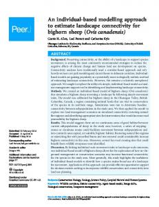
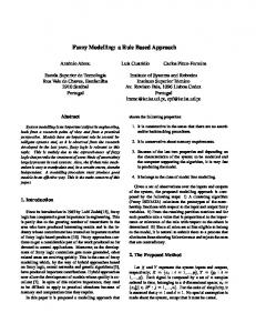
1.3 THESIS LAYOUT In order to meet the objectives of the study, a research framework was developed. The following paragraphs explain the research framework and the layout of the work presented in this thesis. A graphical representation of the structure of the thesis is given in Figure 1.1.
Chapter 2 provides the background to the issues in rural transportation planning in developing countries. It analyses the existing methodologies and draws conclusions regarding the gaps identified and the way forward to cover these gaps. It establishes the need to develop a rural travel demand model.
Chapter 3 reviews the basic concepts of accessibility of activities as the basis to represent individual travel behaviour in the context of participation in activities. The two broad modelling concepts reviewed are accessibility analysis and activity analysis. This forms the basis for development of a travel behaviour modelling framework by incorporating accessibility analysis in an activity-based framework.
Chapter 4 deals with the development of the rural travel demand modelling framework. It explains the basic concepts used and derives the mathematical forms for modelling various stages of the framework.
3
Chapter 1: Introduction
Chapter 1: Introduction BACKGROUND Chapter 2: Rural transportation planning in developing countries •Issues in RTP •Existing methodologies •Research needs
Chapter 3: Modelling individual activity-travel behaviour •Accessibility and activity approaches •Modelling systems •Rural accessibility planning models MODEL DEVELOPMENT Chapter 4: Rural travel demand modelling framework •Underlying concepts •Framework stages •Modelling system layout
Chapter 5: Experiment design •Data requirements •Survey design •Data collection
Chapter 6: Analysis of rural activity-travel behaviour •Description of study areas •Household travel decision economics •Individual activity choice analysis
Chapter 7: Development of a system for modelling rural travel demand •Mathematical development •Model calibration •Worked example
Chapter 8: Model application •Case studies •Model verification •Sensitivity analysis
Chapter 9: Conclusions and recommendations
Figure 1.1 Research framework and thesis layout
4
Chapter 1: Introduction
Chapter 5 describes the experimental design for the field data collection exercise carried out from representative rural locations in Pakistan. It includes the results of a pilot data collection from the same area, and develops a questionnaire for detailed data collection.
Chapter 6 studies the activity-travel behaviour of rural households by analysing the data collected from the rural locations of Hala and Khuzdar, Pakistan. The aim of this analysis was to validate the conceptual framework and to provide inputs for model development.
Chapter 7 presents the development of a travel demand modelling system. The mathematical development of discrete choice models is explained. Alternative logistic regression models were developed and calibrated using the database developed from the household survey. Aggregate demand prediction is carried out using the models developed, and statistical inference is used to discuss model prediction results. A worked example explains the model development procedures.
Chapter 8 describes the model application and sensitivity analysis. The models developed using the data from Hala are applied for the Khuzdar data. Important conclusions regarding model capabilities are drawn. This chapter includes sensitivity analysis of the key model parameters in order to validate their application in various scenarios.
Finally, Chapter 9 concludes the research and outlines the recommendation for enhancing model applications
5
An accessibility-activity based approach for modelling rural travel demand in developing countries
CHAPTER 2
RURAL TRANSPORTATION PLANNING IN DEVELOPING COUNTRIES 2.1 EVOLUTION OF RURAL TRANSPORT PLANNING PERSPECTIVE The perspective of rural transportation planning in developing countries has changed from a ‘road-and-car’ approach to a ‘needs-led’ approach (Howe 1996). The first approach, which continued till the 1980s, focused on the rural transport network and assumed that motorised transport is capable of handling all transport needs of rural households. In the second approach (since 1986), transport was seen as a component of an overall system serving the needs of the rural population (Dawson and Barwell 1993). This change of perspective occurred as a result of a series of concerns on the rural transport interventions in developing countries that failed to bring about the expected developmental benefits. It was realised that a major component of rural travel, namely the off-road network, cannot be addressed using the first approach (the road-and-car approach). The second approach (the needs-led approach) although still in its evolution stage, has been able to provide improved insight into the actual development needs and benefits from the data at the base level. The requirement remains to develop an analytical formulation and a comprehensive planning model.
2.2 RURAL ROADS AS FACILITATOR OF ACCESS There is a basic lack of understanding of defining the actual role of rural roads in the overall road network hierarchy in developing countries. Hine (1982) recognised the role of rural roads in providing basic accessibility, and found that personal travel constitutes the highest proportion of rural travel demand. As such, better access to rural roads can increase the demand for passenger movement. Considering the evaluation of benefits, 6
Chapter 2: Rural transport planning in developing countries
Hine (1982) stated that the current methodologies give high weighting to income, but ignore other dimensions, namely, social change (such as healthcare, education, and political development).
The migration of rural populations into areas of better road access reveals the inadequate access in the areas of their origin. The reason for very low travel on rural roads is incomplete access provision. For example, walking is preferred for the whole journey because an unconnected road results in an unjustifiable transport cost for the partial journey using other modes of transport. The role of rural roads in providing opportunities to the local population to obtain better output for agriculture, reducing the sense of isolation of the rural populace, and improving living conditions and services must be given due consideration in the overall planning of rural roads (Tingle 1977).
2.2.1
The users and non-users in rural transport
The first step towards identification of rural transportation system requirements is to establish an interaction between land-use and transport. In the absence of any suitable sampling frame for carrying out survey in rural areas of developing countries, roadside traffic counting and interviewing provides the starting point for rural transport demand estimation (Howe and Tenant 1977). Household surveys, on the other hand, could be non-representative because households lack cohesiveness and also because of the semipermanent migration of important household members. Howe and Tenant (1977) derived land-use-transportation interaction from roadside interviews on the basis of a predetermined land-use category system. They developed trip generation equations based on significant land-use factors. They found that vehicle ownership is the fundamental unit in trip making. Market trips by a large rural population are dependent on the provision of services by a few vehicle owners. This leads to the conclusion that rural individuals unable to meet the ‘demands’ of vehicle owners (travel fare or timings) are only left with the option of not making the trips. The study, being based on transport users, presumably did not take account of a large number of the non-users of the transport (Howe 1996).
7
Chapter 2: Rural transport planning in developing countries
A direct example of the neglect of real transport issues can be found from Bangladesh. Barwell et al (1985) reported that in Bangladesh, non-motorised transport (NMT) has a 94% share in the transport sector, while the policies recognising the role of NMT in transport only comprise about 0.004%.
Riverson and Carapetis (1991) identified serious gaps in the work on the subject, noting that most efforts for design and construction of secondary and tertiary roads, mainly for motorised traffic, meet merely about 5% of the requirements of rural travel. The current methodologies fail to address walking and other off-road activities related to travel and goods communication. They suggested the need to incorporate accessibility considerations and the quantification of road-off-road interaction.
Proper attention must be given while considering any change from non-motorised to motorised traffic (Hine 1982). For example, a good riding surface will improve efficiency and reduce operating cost of a cart, considering local norms, culture and journey distance.
2.2.2
Mobility as a determinant of accessibility
Ellis (1996) studied the mobility aspects of rural accessibility. He analysed the effects of the provision of transport services for a given infrastructure in reducing operating costs and enhancing mobility. His research integrated spatial planning and provision of transport services in order to enhance household mobility/accessibility. It was concluded that availability of a variety of transport modes from walking to trucks (present in the Asian countries studied) is responsible for an efficient transport charges infrastructure (Ellis and Hine 1995). Furthermore, this efficient transport charges environment has a very positive effect on household travel (and as a result improves their accessibility), in the sense that with a marginal increase in their income level they can take advantage of the higher technology stage (better transport mode) available in the area. Howe (1995), on the contrary, found that non-availability of low-cost transport modes was a major source of decreased mobility and increased poverty of rural population in Sub Saharan
8
Chapter 2: Rural transport planning in developing countries
Africa. Both these works addressed personal mobility as an important determinant of rural accessibility in least developed countries.
2.3 APPLICATION OF CONVENTIONAL TRANSPORTATION PLANNING METHODOLOGY A considerable research effort has been made in studying rural transport in developing countries in the framework of the conventional urban transport planning (UTP) process that primarily evolved in developed countries (Mekki 1981, Yanuguaya 1983, Banjo 1984, 1988). Mekky (1981) found serious errors in the direct application of conventional UTP approaches to developing countries and recommended seeking relationships between distribution of work places, residential places and accessibility. The major features to be incorporated in a developing country context are non-uniformity of landuse and the multipurpose nature of trips, high population growth, increased rural to urban migration and scarce resources. Models must be responsive to stringent cultural norms. For instance, kinship (family attachment) must be given high weighting for social trips. Although Mekky (1981) focussed on the UTP problems, his arguments are applicable for developing countries’ rural transport problems also. He recommended the use of simple or less complex models to cope with data scarcity. Due to fast changing land-use, incremental models are recommended, i.e. models incremental with respect to the near future.
Yanuguaya (1983) suggested that the modelling approach must be inductive (developed from data) instead of deductive (calibration of existing models). Banjo (1988, 1984), has given an outlook of tailoring the conventional UTP for application in developing countries. The mobility parameters to be added are the lack of access (absence of means to make a trip) and cost of access (affordability without sacrificing). Modal split must consist of a formal motorised component (e.g. cars), an informal motorised component (e.g. a large number of motorcycles) and non-motorised component (animal or human driven vehicle and on-foot travel).
9
Chapter 2: Rural transport planning in developing countries
Except for Mekky (1981), these studies did not perceive that the economics of the transportation system is not transferable to the highly constrained nature of the problems in developing countries.
2.3.1
Economics of rural travel
The current awareness in rural transportation planning for developing countries has given a modified view to the economics of rural transportation; a study of market forces as if people mattered. Howe (1996) developed a case in support of this concept that the conventional transport economics vision (the market place and price) is irrelevant in the context of high monetary and time constraints, prevalent in rural areas of developing countries.
The above argument means that the willingness to pay concept must be revised when dealing with rural transport problems in developing countries. In conventional transport economics arguments, the transport supply (roads, vehicles) is the product and is available to all users in the marketplace (the region). There is an affordable price attached to this product. In the case of rural individuals in developing countries, most people, being non-users, are out of the market place. The new rural transport vision in developing countries must attach a high price to the wastage of time, and develop methodologies based on this concept.
There is evidence in developed countries that need and deprivation provides justification for special transport provisions (Moseley 1979, Howe 1996). The provision of facilities for the disabled may be cited as an example. This argument is the basis of the recent developments in methodologies such as the Integrated Rural Accessibility Planning (IRAP) and Integrated Rural Transport Planning (IRTP), devised for developing countries (details of IRAP/IRTP are given in Chapter 3). These methodologies are people centred and provide a starting point for understanding the economics of rural travel in developing countries (Howe 1996, Edmonds 1998, Dixon-Fyle 1998).
10
Chapter 2: Rural transport planning in developing countries
2.4 CULTURAL AND GENDER ISSUES AFFECTING TRANSPORT LOGISTICS Two important dimensions of rural transportation planning in developing countries to be given due consideration are the issues of gender and cultural norms. Bryceson and Howe (1992) strongly suggested that there is a need to understand how women take part in sharing the transport burden relating agricultural needs, household essential services and childcare, in a multitasking (all in one trip) strategy. Through this, a complete household demand analysis (not only for transport), transformed into agricultural product maximisation could be carried out. Based on findings from Sub Saharan Africa, Bryceson and Howe (1992) identified an important decision chain, composed of three links; namely, cultural norms, land use, and transport. This is important while attempting to model the culturally closed system prevalent in rural areas of most developing countries. They have given examples showing that the transport interventions (in the form of providing cycles to the local people) failed to achieve complete utilisation. This calls for an in-depth understanding of the logistics of local level transportation and all its possible dimensions. The framework suggested could be extended to develop a hierarchy of the overall transportation decision chain.
In recent years concern has been expressed about the effectiveness of rural transport interventions in developing countries in achieving their development targets. This has resulted in a redefinition of the basic approach to the problem (Barwell et al 1985). This revised approach again calls for studying rural transport planning in the context of the needs of local populations.
2.5 RURAL ACCESSIBILITY ANALYSIS It is understood that the real source of deprivation of the rural population is their lack of accessibility to various activities (Barwell 1996). It is therefore necessary to explore this concept in order to have a better understanding of rural transport problems. Moseley
11
Chapter 2: Rural transport planning in developing countries
(1979) provided guidelines for quantifying accessibility and presented various alternative solutions to accessibility problems. He developed a hierarchical transport / land use plan defining area-wise accessibility ratings. Moseley showed that a population potential index could be found, based on the gravity model and the accessibility of a location, which can be quantified in terms of generalised transport cost. Through his work, Moseley (1979) defined two fundamental guidelines for studying rural accessibility: a) mobility: which deals with the transportation solutions to the accessibility problem b) siting of services: which deals with non-transport solutions for the accessibility problem These guidelines are the foundation of the recent work done in accessibility planning in rural areas of developing countries (Barwell 1996).
Among other land-use categories, Howe and Tenant (1977) did not find accessibility to be a significant factor in explaining on-road trips. This leads to a need to investigate the accessibility for the off-road travel. These were the trips that were 'unrealised' due to several reasons. A quantification of these unrealised trips, though, is required for proving this point. It is clear that only an accessibility-based methodology can address this issue. The conventional trip-based methodologies are unable to handle this issue.
Hine et al (1983, 1983a) argued that the provision of basic accessibility, for example replacing footpaths by vehicle tracks, has much higher impact (about one hundred times) than improving the existing accessibility condition (for example, by providing road resurfacing). They concluded that accessibility has a less direct effect on market agricultural production, however, it affects it indirectly through loan financing.
2.5.1
Individual-based approach in rural travel analysis
The common conclusion of a number of studies is that the wastage of time in acquiring access to basic needs and services is responsible for non-achievement of development objectives (Edmonds 1998, Bryceson and Howe 1992). These studies also emphasise that 12
Chapter 2: Rural transport planning in developing countries
transport should be considered in its facilitating role of providing access at a household level.
Recent studies directed specifically at understanding the factors defining transport planning in developing countries, have highlighted concern about the need to address the transportation needs of rural individuals (Barwell 1996, Howe 1996). It is now possible for these findings to be utilised in the methodological development of rural transport planning techniques (Sieber 1998, Odoki 1992).
Moseley (1979) provided an insight to the rural accessibility problem and developed a general framework for incorporating accessibility into rural transport demand generation. A measure of difficulty (or unpleasantness) of making a trip must be converted into a generalised cost function. The central focus, Moseley (1979) suggested, must be on ‘opportunities’ not behaviour.
The missing links in rural travel analysis are the individuals, both in the form of users and the non-users. The conventional methodologies tried to study the transportation system without due consideration of its users and especially its non-users.
Research by Odoki (1992) recognised these missing links and developed rural transport planning methodologies incorporating the individual level analysis. Odoki showed that the household-level needs-based accessibility analysis is able to address both users and the non-users through the same framework.
2.6 RESEARCH DIRECTION There is a need to form a link between classical accessibility research as proposed by Jones (1981) on the development of the accessibility framework, the complementary work by Hine et al in Ghana (1983, 1983a), and the more recent Integrated Rural Accessibility Planning (IRAP) study reported by Howe (1996). While Jones has put in
13
Chapter 2: Rural transport planning in developing countries
place a mathematical foundation for the accessibility approach, the other two works (Hine et al 1983, 1983a, Howe 1996) define practical implications of providing access by studying two aspects of rural access exclusively for developing countries, namely; agricultural production and personal travel. An important area that needs attention is the development of a travel demand methodology, being a key input to the whole transport planning system.
Transport should be considered in its facilitating role of providing access that must encompass all the basic needs and services. It is understood that the real source of deprivation of rural populations in developing countries is their lack of accessibility to various activities. It is therefore essential to explore this area to have a better understanding of rural transport problems.
2.7 SUMMARY The first step towards analysing the rural transportation planning problems is to develop a basic definition of rural transport problems in developing countries (Hine 1982). Other important steps include an understanding of the primary issues (Howe and Tenant 1977), in the light of the real transport logistics of the rural population of developing countries (Bryceson and Howe 1992). There have been concerns regarding the application of conventional urban transport planning models for the scenarios in developing countries (Mekky 1981, Yananguaya 1983, Banjo 1988,1984). This reveals that the basic issues in rural development planning are unresolved, as the problem resides not with the provision of the transport system (Hine 1982), but with the accessibility of activities (Moseley 1979, Odoki 1992). The off-road travel patterns using more logical modes must be incorporated in rural travel analysis. Identification of all forms of non-motorised transport (NMT) and intermediate modes of transport (IMT), and their incorporation into models, is needed, along with the motorised component (MT). Models must be responsive to changes from one transport form to others (between NMT, IMT and MT), due to changes in accessibility levels (Riverson and Carapetis 1991).
14
Chapter 2: Rural transport planning in developing countries
The way ahead is to conceptualise the accessibility of activities to the rural population and to utilise it in a rural transport demand-modelling framework. The model must be sensitive to local service infrastructure, cultural norms, monopolistic economy, and gender issues. Lessons must be derived from the failure of high technology interventions in fully transferring anticipated benefits. The contribution of the concepts developed will be an appreciation of the overall rural transport planning for developing countries.
15
An accessibility-activity based approach for modelling rural travel demand in developing countries
CHAPTER 3
MODELLING TRAVEL BEHAVIOUR 3.1 BACKGROUND This chapter first reviews the concepts of accessibility as applied in the analysis of travel demand forecasting. The mathematical forms of accessibility measures incorporating various constraints faced by individuals are discussed. The main objective is to develop a measure of accessibility that is appropriate for application to rural areas of developing countries.
The next stage in development of a behavioural travel demand modelling system is the identification of the activity-travel patterns of individuals. The concepts of activity-based travel analysis are reviewed and their mathematical forms are described. A brief statistical analysis of trip-based data is presented as a case study to justify the direction taken for this research.
The outcome of the chapter is the formulation of an accessibility-activity approach that is suitable for incorporating the constraints faced by individuals when analysing rural travel demand for developing countries. This approach incorporates the accessibility of an activity and participation in the activity within the same framework.
3.2 THE ACCESSIBILITY APPROACH The main focus of this research was to incorporate all factors affecting individual accessibility in a travel demand modelling process. It therefore seemed appropriate to first investigate the concepts relating to individual accessibility and then to establish their relevance for the rural travel demand modelling process envisaged in this research.
16
Chapter 3: Modelling travel behaviour
3.2.1
Basic Concepts
Accessibility is a measure of the potential of an individual (or type of person) at a given location, to take part in a particular activity or set of activities (Odoki 1992). It has three components (Hägerstrand 1970, Burns 1979): (i)
the Transportation component - which deals with mobility
(ii)
the Spatial component - which deals with activity location, and
(iii)
the Temporal component - which deals with the timing of activities.
An Activity is a task requiring travel and time to participate in (for example work). An Opportunity is an activity fulfilling all three components of accessibility.
3.2.2
Accessibility Measures
The measures of accessibility seek to give an operational form to the concept of ease or difficulty of reaching activities. Jones (1981) reviewed various definitions and measures of accessibility. Most definitions of accessibility address some or all of the three components of accessibility with the help of functions incorporating one or more of the following four factors: a) spatial separation of locations b) travel cost c) individual weighted or population weighted opportunity, and d) consumer surplus.
Measures of accessibility use different functions to represent their intended definition and use. These functions are; actual cost or time of travel, generalised cost, individual’s utility and the normalised or population weighted characteristics of opportunity.
Jones (1981) defined six criteria to test the viability of any accessibility measure in the general sense. However, Jones left the final interpretation and use of a measure to be case dependent. There are various factors used in development of accessibility measures, as given by Jones. These factors and their resulting accessibility measures are reviewed here
17
Chapter 3: Modelling travel behaviour
with the intention of testing their relevance to this research. As part of a screening process, Table 3.1 presents these factors in the form of six criteria to be fulfilled:
1. Ability to account for location and characteristics of individuals. 2. Ability to account for location and characteristics of opportunities. 3. Ability to account for connecting transport system. 4. Ability to demonstrate constant accessibility with increased opportunities. 5. Ability to account for changes in accessibility with improved transportation. 6. Ability to demonstrate improved mobility from improved transport for non-users.
Table 3.1 Explanatory power of Accessibility Measures DEFINITION GROUPS
MEASURE TYPE
Network measures Spatial Separation of locations Travel Measures Travel cost of obser-ved or expected trips Combined Spatial Opportunity the individual and Travel possesses Measures Opportunity weighted by average population
Consumer surplus
MATHEMATICAL FORMa
CRITERIA COUNTS FOR MEASURE TYPESb 1 2 3 4 5 6
Aij = f (cij) Ii = ∑j cij Tij ∑j Tij BM=q(x).ak.u(Tk) Hansen:(population weighted) Ai= Pi ∑ j Bj f(cij) Contour Measures: Total Opprotunities =∑ j Bj h(cij) Consumer Surplus: S ij =
cij( 2 )
∫
cij( 2 )
Tij (c)dc
a
General description of Variables: Shaded area denotes criteria fulfilled
b
Abbreviations and Terms used: f (cij) = generalised cost function; Tij= interzonal trips; Aij=accessibility of zone j from zone i Pi = population of zone (from); Bj = opportunities in zone (to) Ii= inaccessibility of zone i H(cij) = 1 if cij ≤ C, and 0 otherwise; where C= the contour value Sij=Consumer's surplus BM = accessibility benefit of an individual for participation in an activity-location k q(x) = transportation component of accessibility ak = spatial component of accessibility u(Tk)= temporal component of accessibility Ai = accessibility index of zone i
The shaded blocks in Table 3.1 denote that the measure is able to fulfil the relevant criteria. The higher the number of shaded blocks the greater the ability of the measure to define the accessibility of activities available to an individual from the point of view of 18
Chapter 3: Modelling travel behaviour
application to rural accessibility analysis for developing countries. A brief description of the measures within each category and reasons for failing to meet some of the criteria are given below.
a) Network measures provide information about the transport network but fail to relate transport to the location of opportunities or the individual. They fulfil only criterion 3. b) Travel measures provide information about observed or future travel but are unable to take into account the resulting travel pattern due to changes in travel cost or the accessibility of the activities as perceived by the individual. They fulfil criteria 1 and 2. c) Combined (network and travel) measures in general satisfy most of the six criteria as they tend to include three prerequisites, i.e. travel, location and the individual’s perception towards an opportunity.
The combined measures include four types; Time-space geography measures, Hansen measures, Consumer surplus measures, and Contour measures (Jones, 1981). These measures are reviewed in more detail in the following paragraphs. i)
Time-space geography measures are able to relate the individual with the
opportunities as well as the connecting transport system. In general they fulfil all the six criteria. ii)
Hansen measures are of two types; one which provides a mapping of all
opportunities available in a zone weighted on the basis of a deterrence function; and the second which weights opportunities on the basis of deterrence function as well as the zonal population. The accessibility index is obtained by summation of all these opportunities. They also fulfil all the six criteria. iii)
Consumer surplus, when used in an accessibility measure, can conceive the
benefits of change in accessibility to the individual and are, therefore, able to reflect the demand for travel (taken as goods in the economic sense). The predicted number of trips Tij are obtained in terms of the trips at origin and the attractiveness of the destination, as a measure of the opportunities. But due to its nature of development, the consumer surplus can only take into account the change in travel pattern, i.e. it is unable to find the
19
Chapter 3: Modelling travel behaviour
proportion of the population not using the system neither before nor after the changes. They clearly violate criterion 6. iv)
Contour measures provide a mapping of opportunities on the basis of criteria
functions (for example, travel cost to the nearest facility). They relate land-use and transportation elements of the opportunity by means of deterrence to travel. However, they do not provide information about how the individuals are affected by this interaction. They are relatively undemanding of data.
From the above discussion it seems that both Hansen measures and the Time-space geography measures are able to meet the six criteria set out in order to test the viability of any measure to completely address the full definition and use of an accessibility measure. The following points cover a more detailed comparison of these two measures in order to assess their performance in addressing rural accessibility problems.
a) Hansen measures provide an aggregate measure of accessibility of the activity (as applicable to the overall population), while the Time-space geography measures are able to address individual accessibility problems. b) In the Hansen measures, time is considered in the form of generalised cost, while Time-space geography measures address time in real terms. It may therefore be argued that Hansen measures are incapable of addressing time constraints binding upon individuals, one of the most important issues to be incorporated in rural accessibility analysis for developing countries. c) The Hansen measures are able to cover few activity types, while Time-space geography measures have the flexibility to address all activity types.
The above analysis leads to the conclusion that Time-space geography measures are more suitable for rural accessibility analysis for developing countries.
20
Chapter 3: Modelling travel behaviour
3.3 TIME-SPACE GEOGRAPHY APPROACH The time-space geography approach is primarily based on the space-time autonomy of an individual as conceptualised by Hägerstrand (1970). Time and space dimensions are integrated to study individual behaviour under constraints.
Time-space geography measures conceive the activity programme of an individual in terms of possibilities to perform activities. Time is viewed both to overcome the spatial separation of activities as well as the constraint on the individual. This is closer to the definition of accessibility that concerns with the opportunity an individual (or type of person) at a given location possesses in order to take part in activities. The ‘time-space prism’ (TSP) of an individual considers time as a fixed constraint on the individual and ‘delineates’ the sequence of activities ‘possible’ during a time period (say a day). Two important elements of time used are the minimum time required by the activity and the maximum time to be spent travelling.
The TSP of a hypothetical rural individual is illustrated in Figure 3.1. The individual is free to move in all directions at a uniform speed v1. The horizontal axis represents space in linear dimensions (for example projected distances) and the vertical axis represents time. This simplified prism gives the total time budget available to the individual (e.g., between 8 a.m. and 1 p.m.). This general prism is then constrained on the basis of some further coupling constraints on the individual (i.e. to be present at certain places at certain times). An example is given to define the basic concepts and terminology used.
Consider a school-going child selected from a hypothetical rural household. In Figure 3.1, a ‘2-D map’ is superimposed on the time-space diagram of this individual. A primary school at location A, having less facilities, is reachable in one hour. Another primary school, having a higher quality of education, at location B, is at a further hour’s journey from location A. Both schools have the same ‘opening hours’ (9AM-4PM). The timespace prism of the child ends in the horizontal direction if he opts to go to any of the schools (shown by lines 'ef' or 'gh' in Figure 3.1). His transport, temporal and spatial
21
Chapter 3: Modelling travel behaviour
constraints, however, will define his ability to reach any of these activities. In other words, his TSP is able to define the accessibility of the activity, namely attending school.
Description of salient points in TSP: ac=Total time budget ef, gh, ij = activity duration at locations A, B and Q, respectively ae, ag, ai = travel from home to activity locations A, B and Q, respectively fc, hc, jc = travel to home from activity locations A, B and Q, respectively
Time 1400 c 1300
f
j
h
1200 1100
d
b
1000 g 0900
i
v1
e
0800 a
Projected Distance
A Primary School (poor quality)
Q
B Primary School (good quality)
Home
Plan
Figure 3.1 Time-Space Autonomy of individuals
3.4 ACCESSIBILITY MEASURES BASED ON TIME-SPACE GEOGRAPHY Time-space geography measures view the activity programme of an individual in terms of taking part in activities. Burns (1979) developed an analytical formulation to incorporate all the components of accessibility, i.e. transportation, temporal, and spatial components, in a single framework. He added temporal dimensions to the conventional ‘spatial-accessibility’ approach, which treated the ability of an individual to reach the
22
Chapter 3: Modelling travel behaviour
activities independent of time constraints (both on the activity and the individual). The underlying assumption is that individuals value opportunities available to them in relation to the time budget at their disposal. Burns (1979) defined an opportunity in terms of three non-negative numbers; the travel distance (x), the attributes of the opportunity (a) and the duration of time (T). He represented an opportunity by means of an ordered triad (x, a, T). Collection of such points creates a three-dimensional space that determines an individual's accessibility space.
3.4.1
Accessibility Benefits model
The accessibility benefit measure proposed by Burns (1979) was improved and adapted for application to rural accessibility planning in developing countries by Odoki (1992, 1998, 1998a). The Accessibility Benefits Model (BM), developed by Odoki (1992), integrates various components of accessibility and defines an accessibility measure for application to rural areas of developing countries. The following paragraphs discuss the salient features of the BM model, its mathematical formulation, and explain its relevance for analysing rural travel demand.
The BM model contains four salient factors:
Distance of activities from the location of individuals: The spatial separation of location of activities and individuals is an important determinant of accessibility of activities to individuals. Transportation is needed to cover the distance. This means that transportation infrastructure is an important determinant in defining accessibility of activities. The transportation component of BM incorporates a generalised cost function that describes the deterrent effect of travel on the individual’s perception of the utility of opportunity on the basis of their income level.
Time for activity participation: In a society with limited time at their disposal, the amount of time available for activity participation needs to be properly addressed. Considering the minimum time required for certain activities (for example work) and the opening 23
Chapter 3: Modelling travel behaviour
hours of certain activities (for example shopping), this is an important factor in defining opportunities to the individuals.
Attributes of a single location-activity: The household assigns weightings to the attributes of spatially separated activities. For example, a household without children would not assign any weight to a primary school. In rural accessibility planning it is important to recognise the attributes of an activity as being a determinant of accessibility. For example, the quality of schools within reach of a local population will determine their accessibility to good education. This is also the basis of the Integrated Rural Accessibility Planning (IRAP) concept, described later, whereby the accessibility of an activity to the local population is the basis of defining development targets.
Relative importance of activity to the individual and the household: Contrary to Hansen’s population weighted opportunities, this approach caters for value weighted opportunities conforming to the individual’s time-space autonomy. An activity fulfilling the physical constraints of transportation and its temporal nature, cannot improve accessibility if it is irrelevant to the individual (for example, Work for a school child). It is important, therefore, to recognise the relevance of activities to the individual within the context of the household in order to develop mathematical forms for the accessibility measures.
BM Components Odoki (1998) integrated the three components of accessibility into a single framework by defining BM as: BM = q( x ) ⋅ a k ⋅ u (Tk )
(3.1)
where q(x)
= transportation component of accessibility
ak
= spatial component of accessibility
u(Tk) = temporal component of accessibility
24
Chapter 3: Modelling travel behaviour
The accessibility benefits measure BM in the above form represents the value weighted mapping of opportunities. These opportunities are activities which individuals desire to perform in order to derive benefit from the activity participation. They have to travel to the spatially distributed activity locations and therefore spend time in two ways, i.e. time for travelling, and time for activity participation. The mathematical form of BM considers the perceived value of time in the following ways: a) generalised travel time b) perceived value of time for activity participation (less travel time)
Generalised travel time a) The generalised travel time is addressed through the function q(x) which has the form: ⎡ ⎛ m 1⎞ ⎤ q ( x) = exp ⎢− ⎜ + ⎟2 x ⎥ ⎣ ⎝ αI v ⎠ ⎦
(3.2)
where m
= the monetary travel cost per km
αI
= the value of travel time per hour assigned by the individual having income I
v
= the speed of travel in km/hr
x
= distance to the location in km
Important points to be noted here are: i)
The value of function decreases with increase in monetary travel cost: this represents the fact that travel costs are considered as deterrence towards travel.
ii)
Higher income would yield higher values of q(x): this is based on the assumption that people with income I will value their time at αI per hour. This results in higher travel benefit for higher income individuals.
iii)
The function decreases as the distance to the activity increases.
Time for activity participation The perceived value of time for activity participation is considered in the form:
25
Chapter 3: Modelling travel behaviour
u (Tk ) = h γ (Tk )
γ
(3.3)
and Tk = τ −
2xk v
(3.4)
where h
= measure of utility per unit time, based on the primary activity
γ
= marginal utility of time available to the individual for the activity participation
τ
= total time budget
The function u(Tk) is the value of the real time available for activity participation, valueweighted by the function γ.
The marginal value of u(Tk) is analysed using the operation: du (Tk ) = γ ⋅ h γ ⋅ Tkγ −1 dTk
(3.5)
The function γ, which defines the marginal utility of time Tk (Odoki 1998), can be analysed by the help of four extreme cases (Burns 1979): a) if γ1 the marginal value of time Tk increases as Tk increases, rendering increased utility of the time of activity participation for the individual. c) if γ=1 the marginal value of time Tk is constant for all values of Tk, rendering a constant utility of the time of activity participation for the individual. d) if γ=0 the marginal value of time Tk is zero for all values of Tk, rendering no utility of the time of activity participation for the individual.
The utility of time for activity participation is therefore a non-decreasing function which means that participation in the activity will render a non-negative utility whenever the
26
Chapter 3: Modelling travel behaviour
time of participation is available, i.e. a zero value of utility if no time is available. The function γ keeps this utility within limits by providing an upper bound to its value.
Activity attributes In addition to the utility of time, the BM model incorporates the attributes of the utility for the individual by the composite function ak, which is defined as: ak = ρ ⋅ ω ⋅ c
(3.6)
where
ρ
= level of activity (for example number of jobs)
ω
= attraction characteristics of the activity in the form of weight attached to the activity (for example primary school has higher weight for child under 15 years than any other individual type)
c
= model calibration parameter (c>0)
In behavioural analysis, the activity attributes have an important role to perform in defining the activity space of the individual in order to access spatially separated activities. That is: a) the level of activity offered by the location, addressed by parameter ρ: this term incorporates the conventional activity attraction measure as a determinant of accessibility b) the weighting attached to the activity, addressed by parameter ω: this incorporates the relevance of the activity within the context of the household role the individual has to perform c) the model calibration parameter c: this incorporates the current level of activities for the whole population or area as compared to the minimum acceptable levels planned
Extension for studying travel behaviour Odoki (1992) demonstrated the application of the BM model for investment appraisal purposes. In an activity-based approach the need to participate in an activity location is the basis of determining travel behaviour. Recognising the ability of the BM model to 27
Chapter 3: Modelling travel behaviour
address individual accessibility constraints within a utility framework, this research extended the application of this model within a travel demand framework. The BM model described above can serve as a proxy to the utility function incorporating all the three components of accessibility, as access is considered the determinant of travel in this research.
3.4.2
Modelling travel using the time-space geography approach
The concept of ‘accessibility of activities’ is the main factor that can assist an analyst to understand rural travel patterns. This means that if the opportunities become accessible, they are able to generate more travel. A measure of accessibility with its transport, spatial and temporal components can therefore be used to quantify travel demand. For example, if a bus service from a village to a town is rescheduled (policy intervention) to suit dwellers at reduced cost (relieving transport constraint), to take them and bring them back at a required time (relieving temporal constraint), the need at the town could be met (relieving spatial constraint). In the real world problem, the provision of a better transport link (an improved track, or a new link) will encourage bus operators to focus their attention to this village (increased service, reduced fares, or both) thus making opportunities accessible to the rural dwellers.
3.5 ACTIVITY-BASED APPROACH The history of person movement research dates back to the 1970s. Hagerstrand’s (1970) time-space prism concept acted as a catalyst, and Kofoed (1970) defined a three stage process to form a conceptual framework for analysing personal travel. In this framework, the first stage is the definition of an individual’s time-space prism (which Kofoed (1970) defined as contact field) represented by a fixed boundary in space and time. This defines the activities available to the individual. In doing so he defined activities as threedimension entities. These three dimensions are: purpose (i.e. type of activity), temporal (i.e. timing duration and frequency of activity) and spatial (i.e. location of the activity).
28
Chapter 3: Modelling travel behaviour
The second stage is the selection of activities based upon the individual’s obligatory and discretionary decisions. The third and final stage is the resulting travel.
Representing the trip-based thinking of the era, Kofoed (1970) proposed the need to understand the activity choice and consequently the time-space prism of the individual through his travel patterns. In his framework, Kofoed (1970) emphasised that the travel pattern of an individual is governed by his mobility status. The concepts of internal and external mobility (developed by Kofoed 1970) are worth mentioning here. The former is defined on the basis of an individual’s household obligations and the latter is defined through his socio-economic status and the availability of the activities.
3.5.1
A Behavioural Framework
Subsequent research by the Transport Study Unit (TSU) team (Jones et al 1983) enhanced the activity analysis concepts and a considerable amount of work has been done on travel demand analysis using the activity-based approach. The concepts were made operational and underwent similar development elsewhere (Kitamura 1988). The activitybased approach developed from this point onwards views travel demand within a behavioural framework and suggests answers to the following questions (Jones et al 1983, Kitamura 1988): •
what are the needs of an individual?
•
what are the opportunities available to him?
•
what are the parameters of the utility on which he desires to involve in an activity?
Jones et al (1983) have provided a framework whereby travel is traced in two dimensions, i.e. space and time; as a result sequencing becomes the key element of activities, hence trips.
A study by Ben-Akiva (1996) on the status of travel demand concepts indicated a change in perspective on the modelling approach, from purely a transportation system oriented approach to the activity-behaviour approach. The basic theme is that the demand for 29
Chapter 3: Modelling travel behaviour
travel is derived from a demand for activities. Ben-Akiva’s framework was based on three points: •
conceptual development must be based on demand for travel explicitly for activities
•
the modelling unit must be an individual considering his household involvement and other constraints, and
•
an activity-based modelling system must be used to integrate the daily activity and travel choice in a single framework.
The above references point out a direction for travel demand modelling where involvement in activities is the prime concern. Considering accessibility as the proximity of activities via the transportation network, a concept could be developed in which accessibility of activities essentially leads to the involvement in activities.
3.5.2
Modelling travel demand within the activity-based approach
The main thrust of the activity-based approach is to analyse and predict how individuals respond to changes in their travel environment, and how these responses are temporally correlated (Jones 1990, Kitamura 1988, Ben-Akiva 1996). The decision making takes its roots from the following processes: •
household needs and role allocation to perform activities
•
scheduling constraints
•
spatial and temporal distribution of activities
The household type dictates the formulation of household needs. The household role allocation is necessary in the transformation of these needs to individual activities. The scheduling constraints refer to the activity participation in a multitasking situation. These constraints are imposed from the spatial and temporal distribution of activities, as well as the inter-personal linkages to perform certain activities. These concepts are applicable to the rural transportation scenario in the following ways: •
Firstly, these concepts recognise the importance of household decision making and the role allocation of household members. For example, not just considering the 30
Chapter 3: Modelling travel behaviour
presence of children in defining household structure, but explicitly appreciating their needs and the resulting activity planning (Kitamura 1988). In this way, the concepts are adaptable to an important requirement as repeatedly highlighted in rural transport planning literature (Bryceson and Howe 1992), namely; the cultural and gender effects in activity planning. •
Secondly, the basis of conceptual development is that the travel is a derived demand, i.e. the demand to participate in activities, while the activities are the result of needs. This way they address not the travel but the needs, while incorporating travel as part of a total daily schedule.
With this premise, the conceptual grounds of the activity-based approach are applicable to the need-based thinking required of rural transportation planning.
3.6 EXISTING ACTIVITY-BASED MODELS
3.6.1
An IT-based model
Ben-Akiva et al (1996) reported the conceptual development of an activity-based modelling system in the light of considering information technology (IT) as an option at mode choice stage. People may consider IT as an option while planning their activity programme. In doing so they proposed the following activity oriented considerations: a)
dis-utility of travel: individuals travel only when the net utility of the activity plus travel exceeds the activities involving no travel
b)
time-space constraint upon individuals: for example returning home or the activity-time budget concept
c)
household context: individual decision as influenced by other members
d)
day to day dynamics of decision making: addressing the variable nature of traveltime and activity duration for activity work
31
Chapter 3: Modelling travel behaviour
They defined a modelling framework hierarchy as follows: Level-1:
Lifestyle decisions (for example participation in the workforce)
Level-2:
Mobility decisions (for example work, school locations)
Level-3:
Daily activity decisions (for example work, school type)
This concept is the basis of the activity-based approach, which is useful for modelling rural travel behaviour in developing countries. The daily activity behaviour is constrained by access needs (time spent in acquiring basic needs) and forces individuals to adjust their mobility decisions (where to work), and ultimately results in migration to less isolated areas (Level-1 decisions).
3.6.2
The HATS study
The Household Activity Travel Simulator (HATS) was originally developed by the Transport Studies Unit (TSU) in the 1980s by Jones et al (1983). It studied travel in the context of household activity pattern, considering travel as a subset of the whole activity schedule. HATS was amongst the first models which provided insight into the activitybased approach. The main procedure is a three-stage process, Motivation-ActivityTravel: a way to understand the motivation of any activity undertaken, in order to model the travel for the activities.
The HATS is a social survey technique, based on exploratory design, which involves three survey instruments (Jones 1980): •
an activity-travel diary; to be filled by the respondents prior to the interview
•
a gaming board (called the HATS board); to physically represent the time-space linkage of activities and travel, and to interactively demonstrate the effects of any changes of individual or activity attributes on the activity-travel patterns
•
an interview / discussion on various options inducing changes in the activity-travel arrangements.
32
Chapter 3: Modelling travel behaviour
By conducting the survey at the household level (with all the family members present), the HATS technique also records the inter-personal linkages between household members and their constraints on travel. Implicitly, it is able to incorporate the socio-economic constraints acting upon individuals, for example, income, car availability, etc. HATS is useful in obtaining a quick response with a higher efficiency than a longer interview if an equal amount of information is needed (Jones 1978). As a simulation exercise, HATS is able to provide insights for development of analytical models of complex household-level behaviour.
The findings of the HATS survey (Jones 1978) are in line with Ben-Akiva’s (1996) threelevel decision hierarchy concept (see section 3.6.1 above). This means that people adapt to changes at higher levels after they fail to adapt any further changes in the lower levels, i.e. long term decisions would be the last to be altered. This leads to the definition of a threshold for change, i.e. what is the perceived level of benefit which will cause changes to any level of decisions. One of the salient features of the HATS technique is the ability to identify the flexibility of adjustment in the household activity-travel pattern. This is the gap to be addressed by the policy options.
The model combines the Spatio-temporal distribution of activities (including travel) with an interview process in order to seek the motivation behind various decisions. This provides inputs to an optimisation model which incorporates the following: •
Maximisation of utility for activity participation
•
Trade-off between household members (household role allocation)
•
Dynamics of adaptation
•
Threshold effects (defined in terms of spatio-temporal constraints, which is the same concept as coupling constraints by Burns (1979))
In the context of this research the HATS model provided an insight in designing the social survey carried out from rural areas of Pakistan. Its direct applicability is questionable to the extent that the illiteracy of the respondents would not necessarily yield the desired results. 33
Chapter 3: Modelling travel behaviour
3.6.3
HATS Application
The Technique The HATS interview is composed of two parts. In the first part, the individual represents his/her existing travel pattern on the HATS board. For a working individual, a simple HATS board for a typical working day might look like Figure 3.2.
Time
Hours
8
8
8
8
9
9
9
9
17
17
17
17
18
18
18
18
Minutes
00
15
30
45
00
15
30
45
00
15
30
45
00
15
30
45
W
Out of Home Activities
W
W
W
W
Sh
Travel Home Activities
S
E
E
E
S
S
S=Sleep E=Eat W=Work Sh=Shop
Figure 3.2 HATS Board for the hypothetical example
In this way the HATS board is able to identify: a) types of activities in which the individual is involved in b) activity and travel patterns in time-space co-ordinates
Ability to predict behaviour The HATS technique is developed to be used in the form of a time series information collection instrument. It is done by inducing the intended policy in the individual’s activity-travel pattern. The individual is required to adjust his/her activities/travel and reach a point of equilibrium where no more adjustment is possible. This will provide the following information about the individual’s activities: a) fixed activities (activities which can not be adjusted, for example work) b) flexible activities (activities which have some margin of adjustment, for example sleep, eat, playing etc.) This information is used to predict travel behaviour under similar policy interventions.
34
Chapter 3: Modelling travel behaviour
Extension to Rural Transportation Planning in developing countries Addressing the time-space constraints upon individuals is the basis of the HATS technique. This provides a suitable starting point for studying rural accessibility problems in developing countries. Furthermore, HATS can also address household level analysis to be carried out to study activity behaviour. It therefore becomes an appropriate tool for studying rural travel demand. A research effort is needed in order to develop a simple household level travel analysis incorporating the following more explicitly: •
travel as a source of high burden on time
•
the cultural and gender issues
3.6.4
The CARLA Model
Developed by the same team as HATS, the CARLA model is considered to be more comprehensive than HATS (Garling et al 1994). Its main advantage is its ability to simulate a large number of alternative schedules so as to deduce more definite results about actual behaviour.
CARLA includes a computerised algorithm (Knippenberg 1984), the input of which is the processed information from activity-based diaries. The algorithm performs two tasks: a) calculates earliest start time (EST) and latest finish times (LFT) for each activity, and b) provides possible rescheduling combinations using EST and LFT.
3.6.5
An activity-based choice model
Kitamura (1984) developed an activity-based choice model, in the context of discretionary activities. It closely follows the utilitarian approach to time allocation. The main theme was that a discretionary activity will be chosen only if it improves the total utility for the individual, and time allocation for the activity participation was done accordingly. The activity choice and time allocation were, therefore, considered in the same framework. The utility function was non-zero only for those activities to which the individual has allocated any time. Considering the discretionary activities, Kitamura 35
Chapter 3: Modelling travel behaviour
argues that their marginal utility diminishes as the amount of time allocated increases. In this way there is an optimal time for each activity, as illustrated in Figure 3.3.
Utility
Time
Figure 3.3 Activity duration and utility
The conceptual basis of this viewpoint was as follows: a) although the activity duration is considered continuous on the time scale (Jones, et al 1983), the discretionary activities must be treated as discrete entities b) this affects the perceived importance of time allocation and the calculation of utility of the activity.
3.6.6
Application of activity-based approach to rural travel studies
It may be concluded that the existing activity-based models consider time as a prime factor in developing the utility of activity schedules for individuals. They are suitable for policy studies aimed at relaxing time constraints for the individuals.
In view of the application to the RTP, it may be argued that the modelling approach must also consider the availability of the activities to the individuals. This is only possible through the concept of accessibility.
The mathematical form for the accessibility measure relevant to this situation must be able to: 36
Chapter 3: Modelling travel behaviour
a) define availability of activities to the individual by recognising both the spatial and temporal dimensions of the activities as well as the household level weighting; b) incorporate time in two forms, as dis-utility of travel as well as the time for activity participation.
3.7 THE ACCESSIBILITY-ACTIVITY APPROACH The opportunities, which require participation in the spatially distributed activities, define the travel pattern of an individual in a given period of time. The time-space prism, Figure 3.4, shows the activity-travel sequence of an individual starting and ending at times A & B, respectively. It can be seen that the activity-space is rearranged after the individual participates in an activity. Three ‘successive’ positions of the activity space, as a result of four activities, are generated in the figure. The travel between activities defines trips. Their sum defines the travel pattern of the individual in one day. In Figure 3.4, the inclined lines show the instantaneous positions of the space-time prism available to the individual after he decides to participate in any activity (the vertical lines). The arrows show trips at the maximum uniform velocity.
Time
B
q
p
o
n
m A
Space
Figure 3.4 Time-Space Distribution of Activities and Travel 37
Chapter 3: Modelling travel behaviour
Integration of the two concepts, the accessibility of activities and the activity-behaviour, provides a better understanding of person movements for application in rural travel demand modelling in developing countries. This is referred to as the accessibility-activity approach and is developed further in the present research to model the rural travel demand.
3.7.1
Integrated Rural Accessibility Planning
The Integrated Rural Accessibility Planning (IRAP) methodology was initially developed for Tanzania and Malawi (initially called Integrated Rural Transport Planning, IRTP). The IRAP is a local-level planning tool aimed to optimise the infrastructure investment on the basis of the most urgent needs of the local community (Howe 1996). This way IRAP is based on the accessibility-activity approach as described earlier, i.e. it takes into account the access needs of households and the activities fulfilling these needs.
In its basic sense IRAP is able to address household accessibility problems. It provides input to the rural accessibility planning process in the form of rating of needs on the basis of household requirements for access as well as the rating of infrastructure on the basis of its ability to provide access. These inputs are used to formulate strategies to reduce access problems in the most optimum budget requirements.
The main feature that IRAP possesses is its flexibility to solve traditionally considered transport-sector problems by either transport or non-transport means. For example, if water collection is a severe access need, the problem can be solved either by provision of better footpaths or roads leading to the facility, or by bringing the water collection points closer to the users. In this way, the IRAP is able to incorporate the mobility and siting of service into the same framework.
The salient features of IRAP framework are (Howe 1996): -
it is needs-based in the sense that it covers all aspects of household needs
38
Chapter 3: Modelling travel behaviour
-
it is comprehensive in the sense of its ability to suggest solutions to the access problems, not just transport problems
-
3.7.2
it is sustainable because it is intended to be managed by local-level participation.
The IRAP methodology
The IRAP methodology is based on household needs for access (Edmonds 1998, DixonFyle 1998). The methodology starts from household data collection. The main aim of the first stage of IRAP (the data collection) is to identify household needs for access to services like water and firewood collection, healthcare, education, etc. Various indicators are used to define the access needs for these services. The time or distance to the facilities offering these services is the main item in the data collection. The IRAP methodology provides two main outputs, the accessibility indicators and the accessibility profile, as explained below.
Accessibility Indicators The first output of the household data collection exercise within the IRAP framework is the development of Accessibility Indicators (AI) for each of the access needs. In mathematical terms, AI is given as: AI = number of households × time (or distance) to the facility
(3.7)
In the above equation the number of households is representative of the population affected. The time (or distance) to the facility is representative of the burden to be borne by the population. The higher the value of AI the least will be the accessibility of a particular facility to a given population. In this way the AI defines, in empirical terms, the inaccessibility of the activities. Parameters other than number of households can also be used in the AI. Table 3.2 explains the range and importance of the parameters defining AI. It contains the definition of AI at various levels of rural accessibility planning.
39
Chapter 3: Modelling travel behaviour
Table 3.2 Examples of Accessibility Indicators VILLAGE Number of households × Water
Ave. collection time in the dry season
Number of households × Health
time to a health centre or clinic
Number of primary school Education
age children × time taken to get to the school
DISTRICT
NATIONAL
%age of households with no %age of households with no direct direct1 access to a water access to a water supply × supply × Average collection Average collection time in the dry time in dry season %age villages
of
season
households with
no
in
health
centre × Average time to a health centre2
%age of households living in villages with no health centre × Average time to a health centre2
%age of households with no %age of households with no primary
school
in
their primary school in their village ×
village × Pupil/classroom Pupil/classroom ratio (or Pupil/teacher ratio)
ratio
(or
Pupil/teacher ratio)
1
Direct access means that water is available in the immediate vicinity of the household
2
Other health indicators would be: regular visits by a Midwife and Physician
Source: Edmonds 1998
From Table 3.2 it is clear that the definition of AI is based on two factors: a) the effected population; for example households or number of school age children b) the burden; for example time taken to the facility or the distance to be covered
In this way the AI defines two possible ways of the solution to the access problem: i. by reducing the size of the effected population; this can be done by improving the capacity of the facilities (increasing number of classes, etc.) ii. by reducing the distance or time for access; this can be done by improving the infrastructure (provision of roads) or enhancing supply of transport vehicles (IMT, NMT, etc.)
Accessibility Profiles The accessibility indicators AI are used to develop accessibility profiles of the areas covered in the IRAP study. These are the maps of the whole area under study redrawn to highlight the access problem of locations (for example villages) with reference to the
40
Chapter 3: Modelling travel behaviour
burden they face. The accessibility profiles act as the planning tool in guiding the decision-makers regarding the most optimum use of the resources.
3.7.3
Utilisation of IRAP concepts
The IRAP model as described above is a local level-planning tool. It’s capability to provide data on household needs and subsequent strategy development can be enhanced by linking it to the travel demand modelling framework developed in the present study. A brief structure of this procedure is explored in Figure 3.5. This would result in better and up-to-date analysis of accessibility situations.
IRAP is a planning tool but can be enhanced and utilised in the development of an analytical travel demand framework in the following ways: 1. The household need identification concept recognises the derived nature of travel. This can be further improved to model household travel behaviour using access needs of households, an essential data input from the IRAP procedure. 2. The IRAP provides the definition of accessibility on the basis of household and activity attributes. This concept misses out the actual decision-maker, i.e. the individual. There is a need to add the individual in the formulation of accessibility problems. This will enhance the behavioural basis of the IRAP framework.
The research reported in this thesis is aimed in this direction. It brings household needs, their travel decisions and the activity attributes within the same framework, based on the accessibility-activity approach.
The framework proposed in Figure 3.5 shows that the accessibility database can provide inputs to the travel demand model. The travel demand model predicts activity choice and the resulting travel demand, which may be used as inputs at the IRAP stage concerned with strategies to address access problems.
41
Chapter 3: Modelling travel behaviour
IRAP Steps1
Travel Demand Model Stages
•DATABASE •NEEDS ALLOCATION
1. Planning Objectives 2. Planning procedures and targets 3. Define access needs 4. Data Collection
•ACTIVITY CHOICE
5. Produce Accessibility Database
•TRAVEL DEMAND
6. Define Access Problems
7. Strategies to address access problems
8. Prioritise 9. Consolidate 10. Monitoring and evaluation
1.
Source: Howe (1996)
Figure 3.5 Integration of IRAP within a travel demand modelling system
3.8 CASE STUDY: ANALYSIS OF TRIP-BASED DATA This section deals with the analysis of household data collected from a selected rural location in Pakistan during the course of this research. The case study was designed to assess the ability of the trip-based approach to address the household decision-making process. The main objective was to be able to use the outcome of the analysis to guide the direction of travel demand analysis for this research, and to use the resulting data in the development of rural travel demand models. 42
Chapter 3: Modelling travel behaviour
Specific objectives of the case study included assessing the ability of the trip-based approach: a) to identify factors governing household travel demand, with reference to accessibility of activities b) to address household needs formation and the resulting travel to fulfil these needs c) to incorporate constraints on individual time budget d) to develop travel demand models incorporating various factors affecting household travel for access
3.8.1
Study area
The study area was situated in Balochistan, the south-western province of Pakistan (see map of Pakistan; Figure A-1, Appendix A). The area selected was Khuzdar, located in the central part of the province (see location maps of Khuzdar, in Figures A-4, and A-5 of Appendix A). The basis of the selection of Khuzdar was that it represents an area where the overall road access is poor due to dispersed population patterns (a feature of the province of Balochistan).
3.8.2
Survey design
The experiment was designed to collect household level data on the following parameters: •
Household parameters:
income, size (number of persons), vehicle ownership
•
Trip parameters:
number, duration, length (distance), purpose, mode
3.8.3
Data analysis
Data was collected at five locations within the area. These locations were selected as they exhibit variation in population settlements. The data for all these locations combined together gave a sample size of 139 households. Table B-1 of Appendix B contains these
43
Chapter 3: Modelling travel behaviour
data. The data were analysed in order to identify the factors affecting household travel demand, and their implications on the overall activity participation of the household. Consolidated data used in the analysis are presented in Appendix-B.
The variables investigated from the household data were: i)
Income: household income (in Pakistan Rupees denoted as Rs.)
ii)
Household size: HH Size
iii)
Purpose: trip purpose The trip purpose was grouped into five categories as:
iv)
Purpose code: 1
Work, Office
Purpose code: 2
Shop, Farm
Purpose code: 3
Taking
Purpose code: 4
Market
Purpose code: 5
Driving
children
to
and
from
school
Mode: mode used for the trip The travel mode was grouped into three categories as: Mode code: 1
Car, Pickup, Jeep, Van
Mode code: 2
Motorcycle
Mode code: 3
Truck/Taxi
In the listing given above, the trip purposes Work and Office have a fixed duration involvement. Work includes indoor or outdoor working as labour, while Office includes working as an office worker. The trip purpose Shop defines trips to a shop used as the business for the shopkeeper. This trip purpose is therefore the travel to work in the shop either as an employee or as the owner. The trip purpose Farm depicts a trip to attend the farm as a worker or the owner. These two trip purposes represent similar kinds of activities and were therefore combined together into a single category, and assigned Purpose code-2. The trip purpose Driving considered driving as the main source of income.
44
Chapter 3: Modelling travel behaviour
In the travel mode listing, Car, Pickup, Jeep and Van were grouped together as they represented formal motorised modes. These modes were used for a range of distances (see data in Appendix-B). Motorcycle, on the other hand not only represents a highly common motorised mode of transport in Pakistan (not so common in developed countries), but also it is different from mode code-1 due to its inability to be used beyond certain distances. Motorcycle is used for low to moderate distances (see also section 3.8.4). Travel mode Truck/Taxi represents the vehicles used as travel mode by the owners, presumably driving their own vehicles for earning purposes. It must be noted that the travel mode for passengers using a Taxi would be recorded as Car.
Descriptive statistics Table 3.3 summarises the statistical parameters for household data. Figure 3.6 and Figure 3.7 show the frequency distribution of these household variables compared with a normal curve. Discussion of the characteristics follows. Table 3.3 Summary statistics of household data STATISTICS
HOUSEHOLD CHARACTERISTICS Income (Rs.)
Household Size
Mean
8080
11
Std. Deviation
6300
6
Minimum
2500
3
Maximum
40000
30
25
4000
7
50
6500
10
75
10000
14
Percentiles
Income The household income showed a skewed normal distribution (Figure 3.6). The range is between Rs. 2,500 to Rs. 40,000, with a mean of about Rs. 8,000. The skew towards lower values of income can be considered as a logical trend in the income distribution
45
Chapter 3: Modelling travel behaviour
over the population (being a rural area of Pakistan, where the majority of the population lives below the poverty line). The 50th percentile of Rs. 6500 implies that the population has average living conditions. 80
Frequency
60
40
20 Std. Dev = 6300.39 Mean = 8081 N = 139.00
0 5,000
25,000 15,000
35,000
INCOME (Rs.)
Figure 3.6 Frequency distribution of income Household size The household size also showed a skewed normal distribution with a mean of 11 (Figure 3.7). The household size ranges from 3 to 30 persons. 40
Frequency
30
20
10 Std. Dev = 5.68 Mean = 12 N = 137.00
0 3
8
13
18
23
28
HHSIZE
Figure 3.7 Frequency distribution of household size
46
Chapter 3: Modelling travel behaviour
The reason for the high mean in the household size is the extended family system prevalent in these parts of Pakistan. This point was also apparent in the activity-based household survey carried out later from the same area (details presented in Chapter 6).
3.8.4
Travel demand analysis
Using the data on daily trip making, it was possible to analyse the factors affecting household travel demand. Table 3.4 presents the distribution of household trips by purpose. Work/Office was found to be dominant in the trip purposes, with Market the second most important category. Each of the remaining three purposes covered around 5% of the total trips reported. The average overall trip distance was found to be 10 km. The trip purpose ‘Driving’ dominated all trip purposes for the obvious reason that the sole trip purpose of the individuals was driving, or work as a driver. The average distance to Work/Office was around the average distance for all trip purposes. The distance for the trip purpose-3 (Taking children to and from school) was the least with the least average time reported. It means that the schools are available in the close vicinity of the population. Table 3.4 Distribution of household trips by purpose PURPOSE CODE DESCRIPTION 1 2 3 4 5
%COUNT
WORK/OFFICE SHOP/FARM TAKING CHILDREN TO AND FROM SCHOOL MARKET DRIVING ALL PURPOSES
57% 6% 4% 28% 5% 100%
AVERAGE DISTANCE (km) 8.8 13.3 5.0 6.1 45.0 10.0
AVERAGE TRAVEL TIME (hrs) 1.9 2.7 1.6 2.5 12.0 2.6
The above analysis revealed that only the trips outside the area were reported. Work being the most important reason for a person to go outside the village, therefore dominated the trip purpose category. This analysis therefore shows a basic characteristic of the trip-based approach: that the individuals consider the most important task/activity carried out during the trip, and report it as the trip purpose. In this way, the trip purpose
47
Chapter 3: Modelling travel behaviour
like visiting health services is not accounted for, as it does not enter the daily travel behaviour of the households.
The distribution of population by travel mode is summarised in Table 3.5. The Motorcycle was the dominant travel mode. This indicates that the majority of the population has moderate or low income levels because Motorcycles are commonly used in these income classes. Motorcycles are used for trips with distances and travel time below average. Table 3.5 Distribution of household trips by mode TRAVEL MODE CODE DESCRIPTION 1 1 2 3
%COUNT
CAR / JEEP PICKUP / VAN MOTOR CYCLE TRUCK / TRACTOR ALL MODES
20% 16% 59% 5% 100%
AVERAGE DISTANCE (km) 7.1 16.2 6.7 26.9 10.0
AVERAGE TRAVEL TIME (hrs) 1.7 3.1 2.2 10.9 2.6
By dividing the mode Code-1 into two parts (i.e. Car/Jeep and Pickup/Van), it was possible to study the proportion of the population using a pickup/van. These vehicles act as low capacity buses and are commonly used on a commercial basis. Households that do not own a vehicle mostly use the pickup/van. Considering the average distance as well as the average duration of trips by pickup/van, it is clear that people used this mode when travelling long distances, and for longer than the average travel times. This means that households not owning transport vehicles either walked shorter distances or their needs are suppressed. This issue cannot be addressed by a trip-based approach.
3.8.5
Modelling travel demand
Household trips models Linear regression models were developed to predict number of household trips. For this purpose, the trips reported in the data were assumed to be journeys. Therefore, for single journey the number of trips was taken as 2. All trips were assumed to be home-based. 48
Chapter 3: Modelling travel behaviour
In order to analyse the contribution of the trip purpose and the mode of travel in travel predictions, multiple regression models were developed on the basis of individual classes of the two variables. In the household trips models, household income, household size, travel distance and trip duration were taken as the explanatory variables. Total household trips were used as the dependent variable.
The model form used for number of trips classified on the basis of trip purpose was:
T p = β o + β1 I + β 2 H + β 3 x + β 4 t
(3.8)
where:
Tp
= number of household trips per day by trip purpose p
I
= household income (Rs.)
H
= household size
x
= travel distance (km)
t
= travel time (hours)
β0 to β4 are regression constants The model form used for number of trips classified on the basis of travel mode was:
Tm = β o + β 1 I + β 2 H + β 3 x + β 4 t
(3.9)
where:
Tm
= number of household trips per day by travel mode m
other variables are as in equation (3.8).
Model parameters were estimated for equation (3.8) and equation (3.9). Table 3.6 summarises the models selected on the basis of statistical parameters R2, F and t. The coefficient of determination (R2) gives the proportion of the total variation explained jointly by all the variables included in the model (Gujarati 1995). The F-statistic provides the significance level for the model as a whole. The t-statistic indicates the statistical significance of each coefficient in the linear regression model. Table 3.6 reports the Fstatistic for each model along with its significance level in terms of p-value, which is 49
Chapter 3: Modelling travel behaviour
known as exact level of significance of the F-statistic, given as a probability value (Gujarati 1995). For all the models reported in Table 3.6 the significance levels of the tstatistic, of all the coefficients reported, have been above 90% (p≤0.100). This was possible using the backward elimination procedure for estimation of linear regression models in statistical analysis software SPSS. This procedure eliminates all nonsignificant coefficients such that the final model contains statistically significant coefficients only.
Table 3.6 Models to predict number of household trips MODEL FORMS
PARAMETER ESTIMATES2 PURPOSE/MODE 1 CODES Constant Income HHSize Distance
MODEL STATISTICS Time
R2
F
Sig.Level 3
Purpose Code:1
-
5.35x10⁻⁵
0.155
0.019
-
0.806 102.287
0.000
MODELS Purpose Code:2 BASED ON Purpose Code:3 TRIP PURPOSE Purpose Code:4
-
-
0.165
-
-
0.840
36.864
0.001
-
-
Purpose Code:5 MODELS Mode Code: 1 BASED ON Mode Code: 2 TRAVEL Mode Code: 3 MODE
-
-
0.535
-
0.803
16.258
0.016
-5
0.138
-
-
0.738
56.197
0.000
-4
7.11x10
-
2.62x10
-
-
-
0.909
19.993
0.047
-
-
-
0.166
-
0.215
0.793
89.975
0.000
-4
0.106
-
-0.026
0.818 115.452
0.000
-4
-
0.021
-
0.951
0.011
1.96x10 1.44x10
29.283
Notes: 1
Purpose Codes: 1=Work/Office; 2=Shop/Farm; 3=Takingchildren to and from school; 4=Market; 5=Driving. Mode Codes: 1=Car/Pickup/Jeep/Van; 2=Motorcycle; 3=Truck/Taxi.
2
Parameter estimates are reported for the parameter coefficients found to be at or above 90% significance level.
3
p-value for F-statistic; a zero denotes very small value.
On the overall basis, Income and Household size were found to be important variables explaining the trip making at the household level. Travel time was not found significant in any of the models based on trip purpose. This suggests that travel duration does not effect trips for any of the trip purposes considered. Models for the travel modes (mode codes 1 and 2), on the other hand, include travel time as a significant variable. This indicates that the use of a transport mode would be dependent on travel time and in turn affects the trips made by the household.
50
Chapter 3: Modelling travel behaviour
All the eight models for household trips (five purpose codes and three mode codes) have zero intercept value. This indicates that in each of these models certain combination of values may result in no trips made by the household. A simple case to understand is Purpose code: 3 (Taking children to and from school). The distance was the only explanatory variable in household trips by this purpose code. For distances approaching zero, therefore, the number of trips would approach to zero. This may be considered logical in trip-based approach as only trips outside the area get reported. This is an important limitation of trip based approach, that it does not account for the time spend in out-of-home activities.
Trip duration models The mathematical form used for the linear regression model for predicting trip duration on the basis of trip purpose was:
t p = β o + β1 I + β 2 H + β 3 x
(3.10)
where
tp
= trip duration for trip purpose p
other variables are as defined in equation (3.8).
The model form used for predicting trip duration on the basis of travel mode was:
t m = β o + β1 I + β 2 H + β 3 x
(3.11)
where
tm
= trip duration by travel mode m
other variables are as defined in equation (3.8).
Table 3.7 summarises the trip duration models which were found to be statistically significant on the basis of the F and t statistics (explained earlier).
51
Chapter 3: Modelling travel behaviour
Table 3.7 Models to predict trip duration MODEL FORMS
PARAMETER ESTIMATES2 PURPOSE/MODE CODES1 Constant Income HHSize Distance Purpose Code:1
MODELS Purpose Code:2 BASED ON Purpose Code:3 TRIP PURPOSE Purpose Code:4 Purpose Code:5 MODELS Mode Code: 1 BASED ON Mode Code: 2 TRAVEL Mode Code: 3 MODE
-
-
MODEL STATISTICS R
2
F
Sig.Level 3
0.077
0.113
0.476
34.024
0.000
-4
-
-
0.683
15.070
0.006
-4
-
-
0.667
6.000
0.092
2.34x10
2.735
-1.75x10
1.308
-
-
0.176
0.749
119.523
0.000
-
-
-
0.345
0.955
41.993
0.023
-
-
-
0.165
0.723
127.487
0.000
-
-
0.087
0.173
0.595
57.305
0.000
-
-
-
0.344
0.943
66.696
0.001
Notes: 1
Purpose Codes: 1=Work/Office; 2=Shop/Farm; 3=Takingchildren to and from school; 4=Market; 5=Driving. Mode Codes: 1=Car/Pickup/Jeep/Van; 2=Motorcycle; 3=Truck/Taxi.
2
Parameter estimates are reported for the parameter coefficients found to be at or above 90% significance level.
3
p-value for F-statistic; a zero denotes very small value.
On the overall basis, travel distance was found to be a significant factor affecting trip duration. Considering trip purposes, except trip purpose codes 2 and 3, the trip duration was proportional to the travel distance. The distance therefore profoundly affected the trip duration. The factor affecting trip duration by purpose codes 2 (Shop/Farm) was household income. This suggests that higher income households would spend more time in travel to their shops/farms. Income was also the factor affecting trip duration for trip purpose 3 (Taking children to and from school). The negative sign for this coefficient suggests that higher income households would spend lesser time in travel for this purpose. This means that higher income households have access to better transport modes (for example Cars) and therefore spend lesser time in taking children to and from school.
The model for trip duration by purpose code-1 (Work/Office) explained less than 50% of the variation in the data. This indicates that trip duration for Work/Office did not follow a linear trend and the linear regression model of equation (3.10) was unable to address all the variation in the data. Similar argument may be extended to trip duration model for model code 2 (Motorcycle) which explained less than 60% of the variation in the data.
52
Chapter 3: Modelling travel behaviour
Trip duration for either of the three mode classes is proportional to the distance of travel. In the case of mode code 2 (Motorcycle) a joint dependency on household size suggests that larger household size increases the travel duration for these households. This indicates that as the household size increases, there is increased demand on the time budget of the individual (due to increased travel duration). This point, however, was unable to be addressed without a detailed analysis of activity duration as well as daily time utilisation.
3.8.6
Conclusions of the case study
The above analysis of the trip-based data highlighted the following points related to the trip-based approach:
•
Only trips outside the area are reported
•
Trips to reach non-frequent activities like visiting health centres may not get proper reporting as they do not constitute daily trips
•
The analysis of other factors like household interaction is not possible
In the light of the objectives set out for the case study it is concluded that: a) the trip-based approach identified factors related to household travel for activities (for example, household income, household size, etc.); this approach does not address factors related to activities (for example alternative locations of activities, etc.) b) the trip-based approach identified factors affecting travel demand to fulfil household needs (for example Work, Market, etc.); this approach does not incorporate travel to fulfil the household needs which follow a non-daily pattern (for example travel to activities like healthcare) c) the trip-based approach identified the time constraints on individuals with reference to travel to the activities; this approach does not incorporate individual's daily time budget constraints as it does not include activity duration, etc. d) the linear regression models based on trip-based data included explanatory variables at the household level (for example household size, vehicle ownership, etc.); the tripbased approach does not incorporate individual level constraints affecting travel 53
Chapter 3: Modelling travel behaviour
demand (for example role allocation, etc.), required to completely explain household travel for access.
For further analysis, an activity-based approach must be adopted which should study both activity participation and travel within the same framework.
3.9 SUMMARY The conceptual development of a rural travel demand model in developing countries must seek to integrate mobility and accessibility in the same framework. In the accessibility based approach, transport is considered as a component of accessibility of activities. The activities can be mapped in time and space and the opportunities available to the individual can be deduced. This approach lacks the behavioural sense in the way that the participation in an activity cannot be completely determined solely on the basis of the activity being accessible. The activity based approach is able to deduce an individual's participation in activities. This defines the activity pattern of the individual. The travel pattern of an individual is considered as the subset of his overall activity pattern. This approach, however, in its basic sense, does not realise any space-time constraints upon individuals, i.e. the availability of these activities to the individual.
The accessibility-activity based approach is able to integrate the concepts of the above two approaches whereby the activity participation of an individual is a function of mapping the activities in time and space. The accessibility-activity approach recognises travel as a derived demand, a demand to access spatially distributed activities, within the time-space constraints of the individual. The rural travel demand model developed in the present research is based on this approach.
Analysis of trip-based data from a selected rural location in Pakistan was presented as a case study. It was concluded that while the trip-based approach identified various factors related to household travel to access activities fulfilling household needs (for example
54
Chapter 3: Modelling travel behaviour
Work, Market, etc.), it was unable to provide a complete insight into the factors affecting household travel in rural areas of developing countries. This argument calls for development of a framework that integrates travel analysis within activity analysis.
55
An accessibility-activity based approach for modelling rural travel demand in developing countries
CHAPTER 4
TRAVEL DEMAND MODELLING FRAMEWORK 4.1 INTRODUCTION Previous chapters reviewed research on rural transportation planning in developing countries. The literature in general stressed that rural transportation planning concepts must be formulated on the basis of household needs and targeted towards providing the means for fulfilling these needs. Rural travel, therefore, must be understood as the means to access the activities required to fulfil household needs.
This research recognises that household needs are the determinant of rural travel demand, and the subsequent travel to participate in activities is primarily to fulfil these needs. The research attempts to model rural travel demand within a conceptual framework, which integrates the accessibility of activities and the participation in the activities by individuals in order to derive the demand for travel.
This chapter describes the rural travel demand-modelling framework. It explains the underlying concepts forming the basis of the accessibility-activity approach taken in this research to model rural travel behaviour. Various stages of the modelling framework are described together with their operational development.
This chapter further describes the procedures required to carry out each stage of the framework and explains the parameters needed at each of the stages. An empirical analysis of the model parameters is also included to test the behavioural extent of the framework.
The conceptual framework forms the basis for the development of the travel demand modelling system. The outlook of the whole system is presented with the primary tasks
56
Chapter 4: Travel demand modelling framework
and the input-process-output of each component. This is followed by a description of detailed processes and algorithms used in various components of the system.
Figure 4.1 explains the flow of the tasks carried out in the development of travel demand model as explained in this chapter.
Conceptual framework
Mathematical development Accessibility of activities
Threshold limit
Modelling activity choice Explanation of parameters
Mathematical form
Modelling system System modules
Procedures
Figure 4.1 Model development stages
4.2 UNDERLYING CONCEPT People interact in time and space through the activities they perform. Travel is needed to reach a spatially separated activity. The overall activity participation behaviour of individuals during a given time period is indicative of their travel patterns. This concept is used in this research to develop a travel demand modelling system, by answering the following questions that are the basis of the sequential transport planning methodology: 57
Chapter 4: Travel demand modelling framework
• What is the purpose and frequency of trips; i.e. trip end estimation • What are the origin and destination of trips (in time and space); i.e. trip distribution • What is the mode of travel; i.e. modal split.
4.2.1
Household travel for Access
The main focus of this research is the identification of rural travel in the context of household access needs. This is achieved in the following way:
a) Considering the household as the unit of analysis In the current research, travel demand analysis starts at household level. This defines household level needs and the interaction between individuals as household members. It results in identifying the responsibilities of, and subsequent activities to be performed by, each member of the household. In this way, the modelling framework is able to address cultural effects and the gender distribution of activities; two significant issues in rural activity / travel demand analysis.
b) Considering the individual as the decision maker The activities fulfilling household needs have to be ultimately carried out by the individuals, collectively representing the household. The individual is, therefore, the decision-maker in the process of activity choice and participation. The demand for travel is therefore derived from the individual decisions for activity participation.
c) Types of access needs and activities Household needs, and the subsequent activities required to meet these needs, are divided into three types, namely; Primary, Secondary and Tertiary. Table 4.1 defines the activity types on the basis of the household needs they fulfil.
58
Chapter 4: Travel demand modelling framework
Table 4.1 Definition of activity types ACTIVITY TYPES
NEEDS FULFILLED
ACTIVITIES
Primary
subsistence needs
Water / Firewood collection, Healthcare
Secondary
economic needs
Work, Market, Education
Tertiary
Rest and recreation
Family/kinship, Leisure
In a given accessibility situation each type of need imposes a particular set of constraints upon individuals and the activities fulfilling the needs. For instance, the pattern of participation in activity work would be found different from that of going to market for shopping.
4.2.2
The decision process
4.2.2.1 Basic assumptions In order to formulate the rural travel demand-modelling framework, the following assumptions are made: 1. Individuals are members of a household. 2. Individuals being household members are responsible for performing activities fulfilling household-level needs 3. There is a bound on the maximum speed an individual can travel 4. All travel and activity participation are sequential on a time scale; this means that the individual cannot be engaged in two activity-locations at one point in time, (please refer to Figure 3.4, chapter 3 for details). An activity-location is a location offering an activity. 5. The home is always the absolute origin and the final destination.
59
Chapter 4: Travel demand modelling framework
4.2.2.2 Decision Hierarchy The activity participation decision is considered in this research to be composed of a twolevel decision hierarchy, as illustrated in Figure 4.2. It is stressed here that, as shown in the figure, the individual is the decision-maker, and reference is made to a particular type of activity.
Accessibility of the Activity The first level of the individual decision hierarchy is the accessibility of the activity. This is composed of the description of time-space constraints acting upon the individual in relation to the activity under consideration. The result is the set of all the activities within the time-space prism (TSP) of the individual. This set of activities becomes the choice set for the next stage, i.e. activity participation.
Household
Individual-1
...
Activity Required
Activity Accessible
Trip Threshold Reached
...
Individual-i
Individual-I
Activity not Required
Activity Inaccessible
Trip Threshold Not reached
…..Level 1
…..Level 2
Individual Travel Demand
Figure 4.2 Individual level decision hierarchy used for modelling travel demand
Activity Participation The second level of the decision hierarchy is the decision whether or not to participate in the activity. This decision is determined in this research by the threshold level for the 60
Chapter 4: Travel demand modelling framework
activity. According to this concept, the household would accumulate needs over time and would travel for the activity fulfilling the need only when the time threshold for the activity would be reached. This threshold level (TL) is attached to the generalised cost the household perceives for the activity. The concepts and mathematical development of TL is described later in this chapter. In the context of daily activities, the threshold level has been implicitly considered in the probabilistic choice process.
4.3 CONCEPTUAL FRAMEWORK The conceptual framework for modelling rural travel demand tends to integrate household needs and individual activity decision-making. It has three stages: 1. Needs allocation 2. Accessibility criteria 3. Activity participation Figure 4.3 illustrates the relationship between these stages. A description of these stages is given in the proceeding paragraphs.
4.3.1
Needs allocation
The village and household type formulate household level needs. For example, a village with no direct gas supply might have firewood collection as a household need for most households in the area. These needs are fulfilled by activities that have to be performed by household individuals. Household roles play the main part in allocation of these needs to the individuals. The needs allocation stage recognises the importance of household access needs. It considers the activities required to fulfil these needs which are then allocated to each individual of the household according to their role within the household. Cultural and gender considerations are addressed at this stage.
61
Chapter 4: Travel demand modelling framework
Population level Database
Household level NEEDS ALLOCATION
Household role allocation
Household needs
Individual level Individual activity agenda Activity attributes
ACCESSIBILITY CRITERIA
Location attributes Activity choice set
Activity threshold reached?
No
Yes Activity location choice
More Activities?
Yes
No
ACTIVITY PARTICIPATION
More Individuals?
Yes
No More Households?
Yes
No Population travel demand
Figure 4.3 Rural travel demand modelling framework 62
Chapter 4: Travel demand modelling framework
4.3.2
Accessibility criteria
As a result of need allocation, each member of the household possesses an activity agenda. Each activity has an accessibility benefit depending upon the attributes of the individual and the activity. Whether or not an activity is an opportunity for an individual is decided on the basis of various constraints acting upon the individual and the activity. As previously defined, an opportunity is an activity that falls within the bounds of the constraints imposed by the three components of accessibility, i.e. the transportation, temporal, and spatial components.
This second stage of the framework determines the availability of activities to each individual, based on the accessibility criteria. This means that each activity, along with the locations providing the activity, is tested on the basis of accessibility criteria to determine whether or not it lies within the time-space prism of the individual and whether or not it requires travel. The outcome of this stage is a set of activities available to the individual, i.e. his set of ‘opportunities’. This set is termed the 'activity choice set' as it contains all the activities the individual desires to participate.
4.3.3
Activity participation
An individual on a daily basis weights all opportunities. The opportunities obtained in the previous stage fulfil two conditions: a)
they are within the time-space constraints of the individual
b)
they require travel
Each activity in which the individual decides to participate determines the individual travel demand. Each activity in the choice set is tested against its threshold level. This was illustrated in Figure 4.2. If the threshold were reached, the individual would participate in the activity, giving rise to their travel demand. The outcome of this stage is the individual travel demand for different types of activities (trip ends), at different locations (trip distribution), and using different modes (modal split).
63
Chapter 4: Travel demand modelling framework
4.3.4
Feed-Back
As illustrated in Figure 4.3, stages 2 and 3 are repeated for all the individuals of the household and then for all sampled households. After completion of all households within the area, the total travel demand for the population sample is estimated by the aggregation of the individual travel demand.
4.4 MODELLING APPROACH The parameters involved at each stage of the travel demand-modelling framework are defined in Table 4.2. The table explains the relationship between stages in the modelling framework and the mathematical modelling process.
The mathematical modelling process first recognises the household access needs through the household type (H) using their Life Cycle Stage (LCS). The household interaction transforms these needs into the activities performed by each individual type (I) in the household. Each of the individual types, therefore, requires a set of activities to be performed, denoted by ( j n ) HI ; n=1,2,3 (types of activities). The activities requiring travel
are assessed on the basis of the attributes of the activity as well as of the locations. This is done through the accessibility criteria. The accessibility benefits model ( BM i ) kj assesses all the activities j at location k, relevant to the individual i. The result of accessibility criteria is the formulation of the choice set of the individual denoted as Ci. From this choice set, the individual will choose an activity-location if the time threshold for the activity is reached. This process is modelled as a discrete choice process with the help of logistic regression models. These models predict the probability of selection of an activity-location in the form of (Pri ) kj , defined as "the probability that individual i will select activity j at location k". This probability density function is used to determine individual travel demand (Ti ) kj , defined as "the choice of individual i towards selection of
64
Chapter 4: Travel demand modelling framework
activity j at location k". The value of (Ti ) kj will always be 1 or 0, defining whether or not, respectively, the choice has been made. The third and final step in the activity participation stage is the aggregation of all individual travel demand to formulate the population travel demand (T ) kj ; defined as "the aggregate demand for activity j at location k". Table 4.2 Parameters of the travel demand modelling framework STAGE
FRAMEWORK COMPONENTS Household needs
NEEDS ALLOCATION
ACCESSIBILITY CRITERIA
Responsibilities upon each individual Activities required to be scheduled by each household individual
DEFINING PARAMETERS Household type (household structure/LCS) Person type (Head, wife, Child) Activity type - Primary - Secondary - Tertiary Individual Activity agenda
MODELLING STEPS
H = Household type I = person type n = types of activities = 1,2,3
( j n ) HI j = one activity of type n
Activity attributes Location attributes
Opportunity -Transportation component - Spatial component - Temporal component
Activity choice set
All activities: - within TSP - requiring travel
Individual travel demand
Activity-location choice
ACTIVITY PARTICIPATION
( BM i ) kj Accessibility benefit: - for individual i, - in participation of activity j - at an activity-location k Ci
Logistic regression models:
(Pri ) kj = probability of selection of a jk-pair Travel demand: For the chosen activity Aggregate travel demand
- All individual types - All activity types - trip purpose - trip frequency - trip timings
65
(Ti ) kj =probability of making trip to an activitylocation (jk)
(T ) kj =
∑ ∑ (T )
k i j
j =1,TJ i =1,TI
TI=all individuals TJ=all activities
Chapter 4: Travel demand modelling framework
4.4.1
Probabilistic choice process
Hensher (1976) proposed the concept of activity node, whereby each activity has three co-ordinates; the time and space co-ordinates and the probability of locating oneself as the third co-ordinate. This three dimensional co-ordinate system completely represents the activity-space of an individual.
Time Time-Space Prism
Distance (a) Unweighted Choice Probability
f(Time, Distance)
Projected Time-space coordinates
(b)
Accessibility-weighted Choice Probability
f(Time, Distance, Activity Attributes)
(c)
Threshold-weighted Choice Probability
Projected Time-space coordinates
f(Time, Distance, Activity Attributes, Activity Threshold)
(d)
Figure 4.4 Probabilistic choice process
66
Projected Time-space coordinates
Chapter 4: Travel demand modelling framework
If the choice probability is represented on the basis of time-space co-ordinates only, then all the activities nearest to the time axis will have the highest probability of selection. The probability distribution in Figure 4.4 (b) should be a normal distribution curve. Since this probability does not give any consideration to the activity attributes, it is referred to here as the 'unweighted choice probability', as illustrated in Figure 4.4 (b). The term unweighted emphasises that no consideration is given to the individual in question or the activity he desires to participate.
A concept of weighted probability is introduced here. This means that if the unweighted choice probability is weighed on the basis of individual and activity attributes, then it will result in accessibility-weighted choice probability, Figure 4.4 (c). Furthermore, introducing the trip threshold and conditioning the accessibility-weighted probability on the basis of the threshold level, then it will result in a threshold-weighted probability, Figure 4.4 (d).
The above concept defines that the choice probability can be modelled as a nested choice where the accessibility of the activity is at the higher level and the trip for the activity is at the lower level.
This research defines the activity-space of an individual comprising of all the activities within the time-space prism of the individual, which have a certain probability of selection. This suggests that each activity within the time-space prism of an individual have some probability of selection, based on the attributes of the activity and the individual. The probability of individuals locating themselves at the activity-location can be analysed as a two-stage process, as explained in Figure 4.2.
4.4.2
Modelling the Accessibility Criteria
The utility of an opportunity is defined on the basis of accessibility benefit of an activity. The accessibility benefit model (BM) developed by Odoki (1992, 1998, 1998a) is used to define the utility function as follows: 67
Chapter 4: Travel demand modelling framework
2x ⎡ ⎛ m 1⎞ ⎤ BM kj = exp⎢− ⎜ + ⎟2 x k ⎥ ⋅ [cρω ] ⋅ h γ [τ − k ]γ v ⎣ ⎝ αI v ⎠ ⎦
(4.1)
where: BM kj = index measure of accessibility benefit.
j
= activity type
k
= activity location
m
= monetary travel cost per km
αI
= value of travel time per hour assigned by the individual having income I
v
= speed of travel in km/hr
x
= distance to the location in km
ρ
= level of activity (for example number of jobs)
ω
= attraction characteristics of the activity in the form of weight attached to the activity (for example primary school has higher weight for child under 15 years than any other)
c
= the model calibration parameter (c>0)
h
= measure of utility per unit time, based on the primary activity
γ
= marginal utility of time available to the individual for the activity participation
τ
= total time budget
This utility function combines the three components of accessibility, namely: •
the (dis)utility of travel, i.e. the transportation component
•
the utility of location-activity, i.e. the spatial component
•
the utility of time, i.e. the temporal component
A discussion on the utility function is given in chapter 3 (section 3.4.1) of this thesis. The following issues are highlighted regarding the application of this function in the travel demand-modelling framework proposed in this research.
68
Chapter 4: Travel demand modelling framework
•
Considering travel as derived demand, the utility function takes into account the travel-related parameters in a negative exponential function. In this way, the BM kj function considers the deterrent nature of travel, which has an exponential effect.
•
A location-activity is characterised by its attributes. This is the attractiveness of a location offering a particular activity.
•
The temporal component in the utility function accounts for the time available for participation in activity after taking away the time for travel.
4.4.2.1 Probability of selection of an activity
The probability (Pr) of an individual selecting an activity j at a location k is given in the form of multinomial logit model as:
Pr( BM ) = k j
exp( BM kj ) ∑ exp( BM jk
k j
( 4.2)
)
where: Pr( BM kj ) = the probability that activity-location ‘jk’ will be selected.
In equation 4.1, the variable BM kj therefore represents the utility of the jk-pair for the individual. Pr( BM kj ) is therefore a relative utility for a given jk-pair over the entire jk-set available.
4.5 CONCEPT OF THRESHOLD LEVEL In a behavioural theory called the Threshold Level Concept, Westelius (1972) found that household needs are accumulated at some rate over time. For each type of need there is a threshold level (TL). When this level is reached, a journey to accomplish that need is 69
Chapter 4: Travel demand modelling framework
triggered (Adler and Ben-Akiva 1979). In this research the threshold level is re-defined to represent the affordability of trip to an activity by a given household type. The TL therefore represents the affordability index for the given household type.
For a household type h and an activity type j, TLhj is therefore defined as a function of generalised time of travel. This generalised time considers both the income and time constraints upon individuals. This concept is applied to model travel demand in rural areas of developing countries.
4.5.1
Generalised time of travel
The household would place a cost of travel on the required activity. This perceived cost can either be given in time units or in money units (Ortuzar 1994). The perceived cost given in terms of time units is called generalised time, i.e. the value of time people place on a given journey. Odoki et al (2000) argued that the generalised travel time, incorporating money and time variables, is able to address monetary and temporal constraints on activity participation, faced by individuals in rural areas of developing countries. They developed a mathematical form for generalised time to be utilised for travel analysis in developing countries, i.e. gt =
m +t αI
(4.3)
where gt
= generalised travel time per kilometre (hrs/km)
m
= monetary cost of travel per kilometre (£/km or Rs./km)
αI
= the value of travel time per hour assigned by the individual having income I (£/hr or Rs./hr)
t
= actual time of travel per kilometre (hrs/km)
70
Chapter 4: Travel demand modelling framework
Two points are worth noting here (Odoki 1992) in the expression of gt in equation (4.3): •
with the income as one of its parameters, the function represents generalised time of travel for a given household type (with a given income level)
•
containing the monetary cost of travel, the travel mode is implicitly selected in the function
One of the assumptions taken into account by Odoki (1992) in development of the function gt was that: "People respond to travel times and costs per unit distance only through the generalised time per unit distance".
This leads to the conclusion that generalised time can be attached to the importance of travel for the individual. In other words, there will be a given gt for each type of activity. Furthermore, Southworth (1981) reported from empirical studies, that the value of time for various activities (including work, shopping and recreation) show a consistent trend. Southworth (1981) found the value of excess waiting time (expressed as a percentage of income) to be 51%, 15.2% and 11.3% for work, shopping and recreation, respectively.
Consequently the following may be deduced: a) gt can be formulated for various income levels and activity types b) as gt has a time component, it can also be related to the TL.
4.5.2
Accumulation of needs over time
Assuming that the needs are measurable in the form of a stock with a given rate of stock consumption, it is possible to represent the level of this stock as a function of time, as illustrated in Figure 4.5.
Mathematically, the consumption stock function Z’ can be represented as a function of time, i.e, (4.4)
Z' = f '(time)
71
Chapter 4: Travel demand modelling framework
Needs Accumulation
Consumption Stock Q
R
Z’
Qmin
Z
TL
Time (a)
Time (b)
Figure 4.5 Need accumulation
If need accumulation can be defined as the reduction of consumption stock over time, then the need accumulation function, Z, is therefore the inverse of the function Z', i.e.:
(4.5)
Z=1/Z'
or (4.6)
Z=f (time)
4.5.3
Needs disbursement
The needs are accumulated until the time when the household participates in some activity in order to disburse them (assumption 2, in 4.2.2.1). The extent to which the needs are allowed to accumulate, is defined as the Threshold Level (TL). Conversely, the TL depends on the time the household can afford to delay carrying out the activity. A third interpretation of TL would be the ability of a household to keep the consumption stock at a given level, Qmin, in Figure 4.5. The concept of TL can be explained with an example. Considering water consumption as a household need, the household requires a given consumption stock at all times. Also, considering that travelling for water collection is the only way to obtain water, the household can delay this travel until the consumption stock reaches a certain minimum level, say Qmin. This Qmin when transformed to the needs accumulation scale is the TL, i.e. the stock level at which the household will make a trip (Figure 4.5).
72
Chapter 4: Travel demand modelling framework
In this way, TL is a function of time and the cost of travel. As it is logical to assume that each need will have a different TL therefore TL must be formulated for each activity type j. Furthermore, the need is a function of the life cycle stage of the household, the LCS
should also enter into the function defining TL. These parameters are therefore incorporated in the function for TL, i.e.:
TLhj = f(generalised time of travel, rate of consumption, storage capacity, LCS)
(4.7)
where j
= 1,2,3
4.5.4
Needs disbursement and threshold frequency
When TL is reached and the trip for the activity (fulfilling the need) is made, the need accumulation is set to zero. The TLs for various activity types intersect the need accumulation function to define the time at which a trip is triggered. The difference can be easily understood by considering a longer time horizon (about one year). Figure 4.6 illustrates this concept. The term Xj defines the number of times the TL is reached and, consequently, a trip is triggered for the activity type j. This is termed as threshold frequency (TF).
According to Figure 4.6 the threshold frequency can be defined as the number of times the threshold has been reached. This whole process is viewed on a one year as the time horizon such that all the types can be accounted for and compared. Three activities are selected to illustrate the concept of TF. The TF defined from Figure 4.6 would then be: (4.8)
TFj= Xj
where TFj
= threshold frequency for the need type j
Xj
= the number of times the needs curve is set to zero by the household.
73
Chapter 4: Travel demand modelling framework
From Figure 4.6, it can be seen that Xj is dependent on the level of the need accumulation when TL was reached. In this way different TLs can be defined for different activities. Thus at a given time horizon 't', X1=4, X2=3, X3=2, giving a total trip frequency of (4+3+2) × 2 trips (per year). Therefore, TF1=4; TF2=3;TF3=2.
Needs Accumulation
TL1 Time X1=4
t
(a) Activity-1 Needs Accumulation
TL2 Time X2=3 (b) Activity-2
t
Needs Accumulation TL3 Time X3=2 (c) Activity-3
t
Figure 4.6 Threshold level and trip frequency
4.5.5
Mathematical form of TL
This section develops the mathematical form of the TL function, in the light of the concepts developed earlier in the chapter. This mathematical development is based on
74
Chapter 4: Travel demand modelling framework
studying how trips for certain activities are carried out. It would then be possible to generalise the concepts for a wide range of activities.
In rural travel pattern analysis for Tanzania, Howe (1996) found that there were only about seven activities that formed a large proportion of rural travel. These activities are given in Table 4.3. Some of these activities and their nature of travel are studied for the development of the mathematical form for TL. Table 4.3 Average annual travel time on some household activities TIME (hrs/year) ACTIVITIES 1 2 3 4 5 6 7
Water collection Firewood collection Crop establishment Grinding Market Weeding Harvesting Reported Total Total of 1-7 as % of reported total Source: Howe (1996)
Female 520 250 200 150 200
1500 88%
Male
200 30 70 50 500 70%
Although the activities presented in Table 4.3 only cover subsistence economic activities, they do however represent 70-88 percent of the overall activity participation. Any models developed on this basis would, therefore, be able to address a large proportion of the rural travel demand.
4.5.5.1 Water and Firewood Collection
More than half of the annual travel by rural women in Tanzania was for water collection and firewood collection (Table 4.3). The following assumptions hold good for both of these activities: a) the activities are part of daily household consumption b) there is a measurable storage capacity for each c) there is a measurable rate of stock consumption
75
Chapter 4: Travel demand modelling framework
The above assumptions are applied to develop the mathematical form of TL in a conceptual model as given in Figure 4.7. It is assumed in Figure 4.7 that the rate of stock consumption has a linear trend. The vertical axis gives the stock level at a given time ‘t’.
Q Qo
TL 0
t (days)
a
Figure 4.7 Parameters defining TL
For a given household the maximum stored stock will be given as: Qo = q o ⋅ H ⋅ a
(4.9)
where Qo
= maximum stored stock available for the household
qo
= average daily rate of consumption per person of the household
H
= size of the household
a
= time (in days) at which stock will fall below TL if consumed by the household at the given rate.
Considering that the availability of the stock is a household necessity, the trip for the activity will be triggered at some minimum level of the stock. This is defined here as the threshold level for the activity. Mathematically: (4.10)
TL = Qmin
and (4.11)
tTL = a
76
Chapter 4: Travel demand modelling framework
where: Qmin
= minimum acceptable stock level
TL
= stock level at the threshold
tTL
= time at the threshold
For simplicity, it is considered that TL represents the zero stock level, i.e.
(4.12)
Qmin = 0
4.5.5.2 Relationship between Threshold Level and need accumulation limit
Based on the above conditions (equations 4.11 and 4.12) the factor 'a' will represent the time taken to reach Threshold Level (TL), where TL is the minimum acceptable stock level (Figure 4.7). Starting from the instance at which the stock was last replenished, the household will allow certain time lapse so that the stock level reaches the TL. In this way, 'a' can be defined as need accumulation limit.
Mathematically the two parameters, TL and a, are related through equation (4.11), i.e. the time at which the stock level reaches a value equal to TL, measured from the maximum stock level Qo.
4.5.5.3 Mathematical form of need accumulation limit
Analysis of equation (4.9) reveals that while qo and H are the physical entities, the term a represents a perceived entity, i.e. the perceived delay for travel to the activity. In this way a accounts for the behavioural component of households travel.
Defined formally, a is “the time which the individual would wait before the next trip to participate in an activity fulfilling a need”. In this way, 'a' represents the perceived value of time the individual would place on the activity in his longer horizon trip scheduling. It is important to recognise that the individuals would perceive the cost of making the trip and would convert this cost into the number of days they would like to wait for the next 77
Chapter 4: Travel demand modelling framework
trip for the activity. Comparing equations (4.7) and (4.9) it is deduced that a is a function of generalised time of travel and life cycle stage of the household, i.e. a = f (generalised time of travel, LCS)
(4.13)
or
a = β (φ g ⋅ x ⋅ g t )LCS
(4.14)
where: a
= need accumulation limit in terms of time to reach threshold, measured from the previous maximum stock level (days)
x
= distance for the activity (km)
gt
= generalised time of travel to the activity (in hr/km)
φg
= factor accounting for the generalised time of travel, representing the number of days of delay in TL per hour of generalised time (days/hr)
β
= calibration factor
The use of equation 4.14 fulfils the following conditions: a) farther activities render higher 'a' values. b) higher gt increases the value of a.
4.5.5.4 Effect of distance and generalised time on need accumulation limit
Figure 4.8 shows how the variation of x, gt and φg affects the trip-making for the activity. It may be demonstrated through Figure 4.8 that higher values of x would tend to sharply decrease the frequency of making trips. This is due to increased gradient of a for higher values of x. Furthermore, in the conceptual model of Figure 4.8 it was assumed that φg is a function of household's life cycle stage. For a given distance the value of a would, therefore, depend on the LCS of the household. For example, for a given distance x, for LCS4 the value of φg would be the least (rendering more frequent trips) and for LCS1 the value of φg would be the highest (rendering less frequent trips) to the activity-location.
78
Chapter 4: Travel demand modelling framework
(φ )
(φ )
g LCS 2
(φ )
g LCS 3
(φ )
g LCS 4
a (days)
g LCS 1
x.gt(hours)
Figure 4.8 Effect of distance on need accumulation limit 4.5.5.5 Boundary conditions for parameters defining TL
The mathematical form of the TL was analysed using some variation on the boundary conditions for the parameters defining TL. These concepts are illustrated in Figure 4.9 (a to d). Figure 4.9 contains four scenarios, i.e.:
a) Households with equal a and variable H (or qo): Equal income households are an example of equal ‘a’. The two households will have the same frequency of trips but will differ in their Qo, i.e. the storage will be different. (Q1>Q2), see Figure 4.9 (a). b) Variable a: The variation in time or distance for travel would result in the variation in a across the population. Households with lower values of a will end up having higher
trip frequencies. Households would also differ in their Qo, i.e. Q1>Q2. This situation is more evident in the case of difference in income level (variable generalised cost) between households. The low income household would have a lower value of a, and higher threshold frequency.
c) Constrained storage capacity: As a special case of (a) and (b) above, consider that the household requiring Q1 is forced to keep it to a lower value, say the storage capacity C, i.e.
79
Chapter 4: Travel demand modelling framework
Qo=C; such that C H2
(Qo)2
a1> a 2
(Qo)2
a2 a
t
a1
(a)
t (b)
Q
Q Qo →∞ C15, Child15 years to be involved in water/firewood collection alongside the housewives.
4.6.3
Accessibility of activities for the individuals
This step involves identification of all the activities that lie within the time-space prism (TSP) of the individual. The activity location and the time required for participation in the activity are needed for this stage of the analysis. It uses two vectors for representing an activity, i.e. {dist}j and {time}j. These are required to completely define each activity j in space and time.
The Activity Schedule
The distance and time vectors are sufficient conditions in the case of discrete activities. However, it is clear that all the activities within the TSP would not be available to the individual if an activity schedule is considered. This means that activities to be performed by the individual must be considered continuous on the time scale, i.e. an interdependency of activities in time and space. The activity schedule can be formed by arranging all possible combinations of activities fulfilling two conditions: activity duration and travel time. This process can be described as: J
τ = ∑t j
(4.15)
j =1
where
τ
= total time budget
tj
= time required for activity j (activity participation plus travel)
J
= total number of activities, comprising the schedule, available to the individual
88
Chapter 4: Travel demand modelling framework
4.6.4
Activity choice
This step estimates the probability of choice of one activity (or schedule) from those activities relevant to the individual type. There are four ways of dealing with this problem.
Firstly, with an empirical approach, the observed choices would be written as a function of certain attributes of the choice. For example, an observed activity can be a function of the characteristics of the individual (income etc.). Field data is used to model the choice process. This approach requires a large number of attributes of the individual in order to replicate true behaviour.
The second approach is to use simulation. The simulation process generates choices on the basis of certain rules. In order to reduce the amount of data to be used in this analysis, it will be necessary to make certain assumptions about the basis of selection/choice. The choice is performed as an optimisation problem using constraints such as time, cost, etc. The objective function will then be the choice of the activity.
The third approach to the problem is the analytical approach, whereby an analogy to certain fundamental principles is developed. A form of this is the econometric or utilitarian approach. The utility function of each feasible activity (schedule) is formed for the individual. The individual is assumed to select the activity/schedule that yields the maximum utility. The economics of decision making is the basis of this approach.
The fourth approach could be considered as a hybrid approach by combining the simulation and the analytical approach. The feasible set of activities or schedules would be obtained from the simulation approach. These are then used as inputs to some utility maximisation process by considering the utility of each feasible activity or schedule.
The proposed demand modelling framework has adopted the following:
89
Chapter 4: Travel demand modelling framework
The accessibility of an activity is considered as the factor defining the feasibility of an activity. Referring to the definition of BM (equation 4.1) given earlier, it is clear that the accessibility of an activity to an individual is defined on the basis of not only fulfilling the time-space parameters but also in terms of the activity attraction parameters. This implies that any activity having a BM less that or equal to zero, would not be considered as an opportunity for the individual. The activity choice is therefore composed of two stages: a) accessibility of activity (or activity schedule) b) probability of selection
These two stages of a choice process can be mathematically given as: ( BM kj )
= f(generalised cost of travel, attraction of activity, time available)
Pr(T jk )
= f ( ( BM kj ) , need threshold)
Explanation of the Activity Choice problem
Consider, for example, a simple case of a housewife from a rural area, whose basic needs comprise three activities, namely; water collection, firewood collection and cooking. This situation is illustrated in Figure 4.12. The figure shows the activity arrangements in time and space. The two prisms a and b are the TSPs for the morning (0800-1200) and evening (1400-1800), respectively.
It is assumed that cooking or preparing a meal from 1200-1400 is a required activity. It can also be assumed that the two activities, although primary activities, can be performed either in the morning 0800-1200 or in the evening between 1400-1800. Due to constrained physical strength, however, the two activities cannot be combined into a single trip.
90
Chapter 4: Travel demand modelling framework
Prism ‘b’
1800
hf
hw 1400
1200
t1
Prism ‘a’
hw
hf
0800
xf
Time
t0
xw
Distance
Figure 4.12 Daily activity pattern of a housewife
The parameters of the activities represented in the figure are: xw
= distance of water collection activity from home
xf
= distance of firewood collection activity from home
sw
= minimum time required for water collection
sf
= minimum time required for firewood collection
hw
= available time for water collection
hf
= available time for firewood collection
sw
(Pr)firewood collection
The above choice process can also be formulated in terms of time available for the activities, according to the time-space geometry as follows: TAM=t1-t0
(4.18)
2xw.(1/v)+hw =TAM
(4.19)
or (4.20)
2xf.(1/v)+hf =TAM
where TAM
= time budget available in the morning hours (0800-1200)
Using this information the time threshold can be incorporated in the utility function (BM) for the activities as:
(BMjk)AM= f[(x,h,T,C)jk ]AM
(4.21)
where (BMjk)AM= accessibility benefit for activity j at location k for the morning hours x
=distance for the activity
h
=time available for the activity
T
=morning time budget for the individual 92
Chapter 4: Travel demand modelling framework
=represents the cost component in the BM function.
C
As C represents the generalised cost function, the timing utility for the activity will be higher in the morning hours. This expression means that the individual would perceive a utility for the activity according to its timing of the participation. On the basis of arguments mentioned earlier, the BM for water collection would be higher in the morning hours than that for firewood collection. The probability of selection of water collection activity will, therefore, be higher than the probability of selection of the firewood activity, i.e. (4.22)
(Pr)w > (Pr)f
4.6.5
Trip frequency
According to the threshold level (TL) concept developed in this research (section 4.5) each activity type will have its TL which will govern the trip for the activity. The function for threshold frequency (TF) will decide the number of trips per year for the activity. When multiplied by the probability of selection of these activities, the trip frequency per year can be found.
Time Horizon
As the mathematical form of TL was developed on the basis of long term needs allocation for the households, the time horizon was considered a year. On the other hand, in order to incorporate coupling constraints, the accessibility criterion uses a daily time budget. It is therefore important to identify the difference of time horizons for the two operations.
This essentially means that two mathematical operations interact at this level: a) probability of selection of an activity (or activity schedule) on the basis of a daily time budget
93
Chapter 4: Travel demand modelling framework
b) frequency of making a trip for the activity (or activity schedule) on the basis of a yearly time horizon
It can be argued that as the probability of an event can be transformed to any scale (time horizon in the present case), it is a valid mathematical operation to find the expected frequency of trip on the basis of a year as the time horizon.
Activity Choice summary
It can be summarised that activity choice is performed as a three stage process: 1. estimating the accessibility benefit of the activity or schedule 2. determining the probability of selection of the activity or schedule 3. determining the frequency of trips for the activity
For an activity schedule, the utility of the most important activity in the schedule would govern. Alternatively weighting of all activities in the schedule can also be considered. The choice in this case would be defined as the choice of an activity schedule out of alternative schedules.
This completes the travel demand analysis for the individual. The aggregate travel demand for the household can be estimated by aggregating individual travel demand to the household and then to the population.
4.7 DESCRIPTION OF MODEL PARAMETERS The parameters governing the accessibility-activity-based modelling framework can be divided into two parts: a)
household and personal characteristics
b)
activity and land-use characteristics
94
Chapter 4: Travel demand modelling framework
The household characteristics are used in the description of household types and the listing of household level needs. The parameters include: -
household income
-
number of children
-
ownership/availability of transportation vehicle
The activity and land-use characteristics used in the estimation of the utility function, and consequently in the activity choice, include: -
location of activities
-
distance of activities
-
connecting transportation system
4.7.1
The activity-related parameters
Three activity-related parameters, are required as follows: a) level of activity parameter: ρ b) a parameter accounting for activity attraction for individual: ω c) a policy parameter: c
4.7.2
The level of activities-ρ
As ρ represents the level or intensity of an activity at a location, it can be expressed in the form of an array of attributes of each location separately as follows:
ρ kj = f {(X kj )l }
(4.23)
where
ρ kj
= level of activity j at location k
(X )
= vector containing attributes of activity j at location k
l
= 1,2,…..L, number of attributes used for activity j
k j l
95
Chapter 4: Travel demand modelling framework
For example, if there are two locations for the primary school with different quality of education, then (X kj )l will represent the quality of education at each location k (here l=1). The mathematical form for ρ is based on the fact that in rural areas of developing countries a large number of households are served by a limited number of activity locations. This fact is addressed by two parameters; namely, the problem index of the activity, and the number of households. Equation 4.24 defines this relationship: PI −1 No. of Households
ψ kj =
(4.24)
where
ψ kj
= attributes of a single activity location
PI
= problem index
The problem index represents the difficulty of reaching the activity in the form of some deterrence function (for example terrain). The parameter ρ can then be found as:
ρ kj = ∑ψ kj
(4.25)
k
From the above two equations, the parameter ρ should be in the form of an array of quality attributes for each activity type with a combined effect of all locations.
4.7.3
Activity attraction parameter ω
In order that ω should define the attraction characteristics of the activity, the following values are taken in the form of weights attached to the activity types: for example, primary=1.0; secondary=0.5; tertiary=0.1; irrelevant=0.001. These weights were assumed for demonstration purpose. Actual values have been derived from field data (as presented in chapters 7 and 8 during model development and application stages). 96
Chapter 4: Travel demand modelling framework
Table 4.7 Activity relevance and weighting for person types Activities
Head
Other
Ch15
Head (Single Parent)
1. Water Collection
0.001
1.000
0.001
0.500
0.500
2. Firewood Collection
0.001
1.000
0.001
0.500
0.500
3. Marketing
1.000
0.001
0.001
0.001
0.001
4. Elementary School
0.001
0.001
1.000
0.001
0.001
5. Secondary School
0.500
0.001
0.001
1.000
0.001
6. Health
0.500
0.500
0.500
0.500
0.001
Legend: primary=1.0;secondary=0.5;tertiary=0.1;irrelevant=0.001
4.7.4
The policy parameter-c
The model calibration parameter c (c>0) represents the development targets to be achieved in the activity levels available to the local population. Possible type of activity listing may be given as in Table 4.8 below (Odoki 1998, Edmonds, 1998). It may be noted in the table that c is actually related to the parameter ρ.
Table 4.8 Example values for policy parameter c Activity
Activities
Type
Activity Level
Existing
Measure
Situation
Target
Value of 'c'
Primary
Employment
Number of jobs
1 per 500
1per 100
100/500
Secondary
Education
Students per school
1 per 250
1 per 150
150/250
Tertiary
Recreational
Number of facilities
1 per 1000
1 per 500
500/1000
4.8 TRIP FREQUENCY The probability of selection of an activity by an individual is based on the accessibility criterion, established prior to this stage. This formulates the probability density function of the activities, which is composed of only those activities: 97
Chapter 4: Travel demand modelling framework
a) that are within the TSP of the individual, and b) that require travel.
TLj, defined for each activity type j, was used for estimating trip frequencies for the given
activity types. The frequency of travel can be found using the threshold frequencies as defined earlier (section 4.5.4). As stated, if this is done on a time horizon of one year, it will give the trip frequency density for one year. According to the basic rules of probability, the expected frequency of the trips made by the individual can be found as follows: (Ti ) kj = TF j ⋅ Pr( BM i ) kj
(4.26)
K
(Ti ) j = TF j ⋅ ∑ Pr( BM i ) kj
(4.27)
k =1
J
{
K
Ti = ∑ TF j ⋅ ∑ Pr( BM i ) kj j =1
k =1
}
(4.28)
where TFj
= threshold frequency for the activity j
J
= total number of activities available to the individual i
K
= total number of locations available to the individual i
(Ti ) kj
= total trips by the individual i for activity j at location k
(Ti ) j = total trips by the individual i for activity j at all locations k offering the activity (Ti )
= total trips by the individual i for all activities j at all corresponding locations k
Equation (4.26) defines the activity-location choice expressed as the probability that an individual would select the activity on the basis of the components of accessibility for the activity at a given location. Equation (4.27) defines the aggregate choice for a given activity over all the locations k. Equation (4.28) defines aggregate travel demand for the individual i.
98
Chapter 4: Travel demand modelling framework
Relating the mathematical development to the four-stage process used in urban transportation planning, it can be showed that: a)
equation 4.26 gives trip distribution, as it preserves trip purpose and trip locations
b)
equation 4.27 gives trip ends by purpose, as it aggregates all locations for a given activity j
c)
equation 4.28 gives trip ends for the selected individual i, all trip purposes and all locations.
4.8.1
Aggregate travel demand
The individual travel demand can be extended to estimate the population aggregate such that: TI
Th = ∑ Ti
(4.29)
i =1
TH
T = ∑ Th
(4.30)
h =1
where Ti
= total trips by the individual i for all activities j at all corresponding locations k
Th
= household travel demand
T
= population travel demand
TI
= total number of persons in a given household
TH
= total number of households in the given population
Considering individual type and household type, the above equations (4.29 and 4.30) would be rewritten as: TI TI = ⎛⎜ ∑ Ti ⎞⎟ ⎝ i =1 ⎠ I
(4.31)
TH TI TH = ⎡⎢ ∑ ⎛⎜ ∑ Ti ⎞⎟ ⎤⎥ ⎣ h =1⎝ i =1 ⎠ I ⎦ H
(4.32)
where 99
Chapter 4: Travel demand modelling framework
TI
= population aggregate travel demand by individual type
i
= one individual of type I
I
= individual type
TI
= total number of individuals of a given type
TH
= population aggregate travel demand by household type
h
= one household of type H
H
= household type
TH
= total number of households of a given household type
4.9 THE MODELLING SYSTEM The individual travel demand modelling stages discussed earlier constitute the rural travel demand modelling system. The modelling system is composed of four modules. Each of these modules consists of processes and algorithms to complete the desired tasks for the module and collectively predict travel demand. Each module is a complete set of inputprocess-output operations designed to perform the tasks required by the module.
The four system modules are:
1. Database module 2. Input vectors module 3. Parameter estimation module 4. Results and aggregation module
The system modules and their tasks are overviewed in this section, and explained in detail in the following sections. Figure 4.13 gives the overall working of the modelling system as well as the details of input, processing and outputs carried out at each modular level.
100
Chapter 4: Travel demand modelling framework
DATA-BASE Village level data
MODEL INPUTS
MODEL ESTIMATION
BM vector for each individual
Multinomial Logit Model
Household level data
MODEL RESULTS Aggregate activity choice
Binary Logit Model
Individual level data Individual activity choice
Observed choice vector
Grouped Regression Model
Figure 4.13 The modelling system
101
Aggregate trips
Chapter 4: Travel demand modelling framework
Database module
This module consists of a number of processes and algorithms developed to process the data obtained from the household survey. The data required may be obtained from various sources such as a purpose-designed survey or published data. The household level data collected from Pakistan, based on the experiment designed to study the rural activity-travel pattern, was the main source data. In addition, use was also made of the aggregate level published information, wherever needed.
The database module integrates the village-level, household-level, and individual-level information to provide the disaggregate data needed for modelling individual travel demand. The output is in the form of a database containing inputs for the various stages of the modelling system.
Input vectors module
The disaggregate data developed at the database stage is used to obtain vectors containing the explanatory variable as well as the dependant variable for each individual. The output from this module is a uniform input for the use by all alternative modelling forms.
Parameter estimation module
The inputs for this stage, the individual vectors, are used in specifying various model forms. The estimation of unknown model parameters is carried out for each model form. The output is the set of model parameters needed to estimate the individual probability of selection of various activities.
Results and aggregation module
Using the set of model parameters obtained from the parameter estimation module, this module first estimates the individual probabilities on the basis of the specifications of the three modelling forms. These individual probabilities are then aggregated, according to the concepts of the relevant model specifications, to obtain the aggregate choice for each activity considered. This aggregate activity choice is utilised to obtain the aggregate travel demand, as proposed in this research.
102
Chapter 4: Travel demand modelling framework
4.9.1
Database module
The database module prepares the source information needed by further stages of the modelling system. It takes the data collected at the household level survey and processes it in order to provide inputs for various stages of the modelling system. The levels of database development and the data processed at each level are: Household level
Household type (LCS) Household activity data (Market, Health, Leisure) Individual level
Individual type (IDs) Individual activity data (Work, School) Village level
Access information for various activities (number of jobs, shops, etc.)
The algorithm for obtaining household type uses the household structure information as its input. It processes the data according to the definition of LCS using Figure 4.14. The output is household type in terms of household life cycle stage (LCS).
Preschool Children NO
YES
School
NO
1
2
Children
YES
3
4
Figure 4.14 Criteria for determination of Life Cycle Stage
103
Chapter 4: Travel demand modelling framework
YES
Is individual the household head?
ID1
NO YES
Is individual the Partner/wife?
ID2
NO Is individual the child over 15 years?
YES ID3
NO YES Is individual the child under 15 years?
ID4
NO Extended Family
ID5
Figure 4.15 Algorithm used to obtain individual type
The algorithm for individual type uses the household structure and the individual identification data. This is applied to each individual of the household. The procedure uses the definition of the individual type, given earlier in this thesis. The output is the placement of the individual into one of the individual types, as illustrated in Figure 4.15.
4.9.2
Input vectors module
Two types of inputs are required for modelling the individual activity-travel behaviour. The input vectors module uses the database as input and processes it to provide the following outputs: BM vector for each individual Observed choice vector for each individual
104
Chapter 4: Travel demand modelling framework
In development of the two types of vectors the following activities are considered: a) Work b) School c) Market d) Health e) Leisure
The BM vector and the Observed vector for each individual contains values for each of the activities considered.
4.9.2.1 BM values for each activity type
The accessibility benefits model BM is defined as the index measure of accessibility of the activity for the individual, as explained earlier. In this way, the BM acts as the explanatory variable for modelling individual travel behaviour. Therefore, the BM must contain all the factors influencing the accessibility of the activity for the individual. This section explains the development of the BM value for each activity type and uses them to explain the procedure to obtain a BM vector for each individual type.
There are three components of the BM model. These are the transportation, spatial, and temporal components. The variables in each of these components are provided with the data from various levels.
A discrete value of BM ij is computed for each individual i and each activity j. The village data provides the input for activity attraction parameters, c and ρ. The household data is used for the parameters important from the point of view of decisions taken at the household level. These parameters are I, ω , h, τ, and γ . The activity dependent parameters are α, m, v and x. Chapter7 and 8 provide the details of how these parameters are estimated using the field data collected.
105
Chapter 4: Travel demand modelling framework
4.9.2.2 BM vector for each individual
On the basis of the methodology for obtaining variables for the BM model, the complete individual level BM vector is formulated using the procedure as explained in Figure 4.16. The procedure takes the data from various levels and uses it in the BM ALGORITHM.
Village level access information
Household Level Data
BM ALGORITHM
INDIVIDUAL BM VECTOR
Individual Level Data
Figure 4.16 General procedure for BM estimation
The BM ALGORITHM is designed to consider the household-level role allocation for each individual type and uses that to formulate an individual BM vector. It is clear that the activities Market, Health and Leisure are regarded as household level activities. Therefore their information is collected at the household level. The activities Work and School are regarded as individual level activities, inferring their information from the
activity data of the relevant individuals. The BM ALGORITHM, explained in Figure 4.17, incorporates the above theme, such that:
a) for the activities Market, Work and School, it takes into consideration whether or not the individual has performed the activity b) for the activities, Health and Leisure, the algorithm considers all household individuals equally in terms of the activity participation.
The output of this process is a BM vector for each individual of the household.
106
Chapter 4: Travel demand modelling framework
BM VECTOR
HOUSEHOLD LEVEL DATA
BM MARKET
YES
Spatial component
Activity attributes
Temporal component
VOT
Transportation component
NO
BM HEALTH
BM LEISURE
INDIVIDUAL DATA
Does Individual perform activity?
Household LCS
BM WORK/ SCHOOL
BM Market=0
All individuals of household
All individuals of household
Does Individual perform activity?
BM Market
YES
Household LCS
Spatial component
Activity attributes
Temporal component
VOT
Transportation component
Household LCS
Spatial component
Activity attributes
Temporal component
VOT
Transportation component
Household LCS
Spatial component
Activity attributes
Temporal component
VOT
Transportation component
NO BM Work/School=0
Figure 4.17 BM ALGORITHM 107
BM Health
BM Leisure
BM Work/School
Chapter 4: Travel demand modelling framework
OBSERVED CHOICE VECTOR MARKET
Does Individual perform activity?
YES
Observed choice in daily activities?
HOUSEHOLD LEVEL DATA
YES NO
Observed choice=1
NO Observed choice=0
HEALTH
Observed choice in daily activities?
All individuals of household
YES
Observed choice=1
NO Observed choice=0
LEISURE
Observed choice in daily activities?
All individuals of household
YES
Observed choice=1
NO
INDIVIDUAL DATA
Observed choice=0
WORK/ SCHOOL
Does Individual perform activity?
YES
Observed choice in daily activities? YES
NO
Observed choice=1
NO Observed choice=0
Figure 4.18 Development of Observed choice vector
108
Chapter 4: Travel demand modelling framework
4.9.2.3 Observed choice vector for each individual type
From the household and individual activity participation information it is possible to derive the individual's observed binary choice for any given activity. The development of an observed choice vector takes data from these two sources and uses the algorithm of Figure 4.18. The output is the binary choice vector for each individual in terms of 0 and 1 (1 for the activity being selected, 0 otherwise).
There are two stages to obtain the observed choice vector. Different sets of steps are carried out for the household activities (i.e. Market, Health and Leisure), and the individual activities (i.e. Work and School). This is achieved in two stages, as described in Figure 4.18:
a) the household activity data provides information as to whether the activity is carried out by the individual on the basis of his/her role allocation. This helps in narrowing down the choice of activities. b) the individual daily activity diary provides the actual observed behaviour of the individual during a typical day.
4.9.3
Parameter estimation module
The choice of an activity by an individual is modelled as a discrete choice process. Three types of specifications have been developed for modelling individual decision-making within the discrete choice approach. Each of the modelling approaches require a set of tasks in order to estimate unknown model parameters based on an observed choice.
4.9.3.1 Multinomial logit model
The multinomial logit model considers all activities and is able to estimate the probability of selection of each activity by the individual. The inputs are the two vectors for each individual; the explanatory variable (BM i ) j and the observed choice vector (Yi ) j . (Detailed explanation of k
(Yi )kj
k
is given in chapter 7). The module uses an iterative procedure as explained in Figure 4.19 109
Chapter 4: Travel demand modelling framework
to estimate the model parameter β used in equation (7.8) in chapter 7. The output is the estimated probabilities of the selection of activities for each individual.
4.9.3.2 Binary logit model
The concept (and therefore the procedure) for binary logit model parameter estimation is similar to the multinomial logit model. The main difference is that the binary choice approach only allows one activity to be considered at a time. The choice is whether or not to select the activity. The algorithm estimates the model parameter β which maximises the likelihood function L(β). The output is the probability of selection of the activity j by each individual i.
4.9.3.3 Grouped regression model
The grouped regression model considers one type of activity at a time. The BM vector for the activity considered is first grouped into N classes. Using the grouped BM vector, and the correspondingly grouped observed choice vector Y jq , the algorithm forms the linear regression model function L*q . The linear regression procedure is then applied to estimate model parameters
β1 and β2.. Figure 4.21 explains this algorithm. Detailed development of the grouped regression models is presented in chapter 7.
4.9.4
Results and aggregation module
The individual probabilities of activity selection are estimated using model parameters obtained as input to this module. The model aggregation relates the travel frequency for a group of individuals using their probability to choose the activity. The aggregation procedure is based on the model definition and specification in each model form. The MNL model, therefore, provides aggregate demand for all activities. The other two model forms provide aggregate demand for the activity for which they are estimated.
110
Chapter 4: Travel demand modelling framework
BM
P = i j
i j
FOR ALL ACTIVITIES: j=1,J
exp( β ⋅ BM ij )
∑ exp( β ⋅ BM mi )
First run?
YES
β = β + inc (Small Increment)
m
Assume β
Y
i j
Report β
NO N
L(β ) = ∏ ∏ (P ) i j
Is y ij
L( β ) < L( β − inc)?
NO
i =1 j ∈ C i
YES
Figure 4.19 Estimation of model parameters -Multinomial logit model
BM FOR ACTIVITY: j
i j
i
P = j
i exp( β ⋅ BM ) j
First run?
Y
β = β + inc (Small Increment)
i
1 + exp( β ⋅ BM ) j
Assume β i j
YES
Report β
NO N
L(β ) = ∏ ∏ (P ) i j
Is y ij
L( β ) < L( β − inc)?
NO
i =1 j ∈ C i
YES
Figure 4.20 Estimation of model parameters -Binary logit model
111
Chapter 4: Travel demand modelling framework
BM qj
Group BM j
BM qj
(Q classes)
FOR ACTIVITY j
Y jq Y
q j
Linear regression
Report
L*q = β1 ⋅ wq + β 2 ⋅ X q*
β1 , β 2
q=1,Q
Figure 4.21 Estimation of model parameters-Grouped regression model
112
Chapter 4: Travel demand modelling framework
4.10 SUMMARY This chapter defined the conceptual framework for modelling rural travel demand in developing countries. The underlying theme was to consider travel to activities fulfilling household needs.
The framework considered the household as the unit of analysis and the individual as the decision-maker. In doing so, it recognised household needs, but the demand for travel was a decision to be made by the individual. The framework combines the concepts of accessibility and activity-based methodologies in order to view rural travel as a result of participation in activities, where the activities available to the individual are based on his accessibility to these activities. The parameters defining each stage of the framework were explained to form the conceptual basis of the framework. Mathematical forms for the framework parameters were developed using behavioural assumptions applicable to rural travel analysis in developing countries.
An important consideration given in this research was the recognition of different time horizons for various decisions. This was defined using the concept of threshold level (TL). The conceptual formulation of functions representing TL was explained. The threshold frequency, defined on the basis of the number of times a household needs to travel for an activity fulfilling a household need, was able to incorporate longer term decisions in the daily travel demand modelling process.
A modelling system capable of carrying out all the tasks at various levels of the conceptual framework was developed. The modelling system is composed of four modules linked together to complete the entire process of modelling aggregate travel demand. The field survey provides the basic data. The database module processed the collected information. This provides information for the input vectors module, which forms the basis of the estimation of model parameters. Finally, the results and
113
Chapter 4: Travel demand modelling framework
aggregation module predicts the aggregate travel demand according to the various discrete choice modelling approaches adopted.
114
An accessibility-activity based approach for modelling rural travel demand in developing countries
CHAPTER 5
EXPERIMENT DESIGN AND DATA COLLECTION 5.1 INTRODUCTION Chapter 4 described the framework for modelling rural travel demand and the variables used in the mathematical development. The next stage is to validate the modelling framework through field data from some selected rural locations. This chapter describes the design of experiments for field data collection.
Basic concepts of conducting social experiments are used to design the rural household survey. The characteristics of rural areas of Pakistan are described to form the basis of selection of locations for field data collection. The sampling parameters are estimated and methodology of their application is described. On the basis of this experiment design, a pilot survey was carried out from Hala, a rural location in Pakistan. The results of this pilot survey provided insight for the detailed field survey. This chapter further discusses the data collection methodology, along with the details of selected locations in Pakistan from where detailed data collection have been carried out.
5.2 DATA REQUIREMENTS The rural travel demand-modelling framework developed in this study was based on a choice process. The choice of participation in an activity is defined as a function of the attributes of the individual and the household. The data collection process must therefore provide the following outputs: a) household attributes b) individual attributes c) activity attributes d) transportation system attributes 115
Chapter 5: Experiment design and data collection
The data items collected were divided into two groups: A. Socio-economic data a. Household level data i.
Household size (number of persons)
ii.
Number of persons employed
iii.
Household vehicle ownership (any transportation vehicle)
b. Individual level data i.
Position (Head, partner, first child, second child, etc.)
ii.
Age
iii.
Occupation and Income
B. Activity participation data a. Activity types b. Locations c. Timings d. Duration e. Frequency of travel
5.3 SURVEY DESIGN The design of a social experiment is parallel to a laboratory experiment with the fundamental difference that the social experiment attempts to represent the design in a natural setting (Moser and Kalton 1971). This means that the basic concepts of treatment and subjects can be extended to the study of human behaviour.
5.3.1
Type of designs
Social experiments are broadly classified as either Descriptive or Explanatory. The descriptive experiments measure the population attributes without consideration of any causal relation between them. The correlation between various attributes may still be found. The explanatory experiments identify possible causal connection between
116
Chapter 5: Experiment design and data collection
variables. The data collection for the validation of the rural travel demand modelling framework requires consideration of both types of experiments. The descriptive experiments would be able to provide the population attributes for various variables and would identify possible correlation among them. The explanatory experiments will be able to identify causal links between various variables involved in the model development. The explanatory type would therefore serve most part of the data collection, which requires inference and validation of the choice process assumed in this research.
The objective of an explanatory type experiment design is to ensure study of all possible causal links between various variables and to minimise the amount and sources of error. Two types of designs of explanatory experiments are relevant in the context of this research; namely: Factorial design and Regression and multivariate design. The factorial design allows for dividing the population on the basis of various factors and studying the effects of each factor on the allocated group. This type of design, although comprehensive, requires a large data collection effort that was not feasible for the scope of the research. The concept of regression and multivariate type of design is that the effect of all possible variables is studied and statistical procedures are used to identify significant variables. This design was appropriate for the current research and was pursued further.
5.3.2
Variables and sources of information
The sources of information were identified for each item of data to be collected. Table 5.1 lists the sources providing data for various parameters of the demand model. For the household variables the source of information was the household head, while data on individual level variables were collected from each individual of the household. Some of the information was obtained from the village/community-headquarter to be used for statistical verification and testing.
117
Chapter 5: Experiment design and data collection
5.3.3
Questionnaire design
On the basis of Table 5.1 the survey questionnaire consisted of three parts; namely, Household information, Individual information and Village information. The questionnaire is given in Appendix C to this thesis. Table 5.1 Data items and sources of information Model Parameters
Data Required
Data Source Household
Individual
Village/ Community
Household Structure and
Size
a
Life Cycle
Income
a
Vehicle Ownership
a
Household Activity,
Activity Types
a
Choice Probabilities
Activity Locations
a
Activity Timings
a
Threshold levels Household Linkage and
Individual Types
a
Roles
Age, Sex, Occupation
a
5.4 SELECTION OF SURVEY AREAS It is important to understand the overall geographical and demographic set-up of the target population in order to plan an adequate data collection exercise. The proposed modelling framework needs to be verified using field data from selected locations of Pakistan. In this context the following points were considered important in order to design a data collection exercise (Hershfield et al 1983, Czaja 1996), applicable for rural areas of Pakistan: a) the administrative spatial set up of the target population: in order to construct sampling frames b) the cultural norms of the population: in order to construct data questionnaires and estimate response rates (and specially the non-response rates).
118
Chapter 5: Experiment design and data collection
The main aim of this research was to study travel behaviour of rural populations. For this purpose the selected location must be classified as representative of rural areas in Pakistan. Pakistan is a federation of four provinces, namely; Punjab, Sindh, Balochistan and the North West Frontier Province (NWFP). In addition there are certain tribal areas directly under the administrative control of the federal government (see Figure A-1 in Appendix A). The Table 5.2 shows that overall, 72% of the population lived in rural areas. Table 5.2 Population and densities of provinces of Pakistan POPULATION (millions)
AREA
DENSITY
(sq.km)
(pop/sq.km)
Total
Urban
Rural
RURAL AREAS
Punjab
47.2
13
34.2
72%
205
230
Sindh
19
8.2
10.7
56%
140
136
NWFP
11.1
1.7
9.4
85%
74
150
Balochistan
4.3
0.7
3.6
84%
347
12
Total (Including tribal areas) 84.2 23.8 Source: Federal Bureau of Statistics,Pakistan (1995)
60.4
72%
796
106
PROVINCES
For the individual provinces, the percentage rural population ranged from the highest in NWFP (85%) and the lowest in Sindh (56%). The province of Balochistan (84%) is close to the NWFP. Comparing the densities of the two high rural concentration provinces (NWFP and Balochistan) the province of Balochistan was selected for the study because it possesses disperse rural settlements (lowest density). Another province selected for study was Sindh having lowest percentage of rural population.
Regarding the population settlements in rural areas of Pakistan, generally a large number of villages are formed around, or served by, a single administrative unit. This is usually the district headquarter or the market centre. This central place generally contains the market, major hospitals, high schools and other major government services which serve the component/surrounding villages, (see also Howe and Tennant 1977 in the case of Kenya). The distance of these villages from the market centre may vary between a couple of kilometres to 10-15 km. This issue was incorporated in the design of the experiment by considering 'cluster sampling' as described later in the chapter. 119
Chapter 5: Experiment design and data collection
5.5 SAMPLE DESIGN Within the framework of a given survey design, the sample design is carried out to ensure the selection of appropriate subjects for study. An ideal sample could be defined as one having the same distribution of attributes as the population from which it is drawn (Fink 1995). This can be achieved, to a great extent, by randomisation.
Three types of sample designs are applicable to random sample surveys: a) completely random design b) stratified design c) cluster design
It is generally understood that the three types vary in their cost effectiveness as well as the accuracy of estimates. The random design is the most straightforward and the cluster design is the most complex of the three. The cluster design is believed to be the most efficient design (Ben-Akiva and Lerman 1985, Stopher and Meyburg 1979). The cost effectiveness of any design should be weighed against the availability of resources for data collection and analysis.
5.5.1
Stratified and cluster designs
Both the stratified and cluster design methods require dividing the overall population into subgroups. In the case of simple stratified sampling, the stratification of the population is done prior to the sampling stage. These strata represent homogeneous units of population (for example men and women). The random samples are drawn from each stratum. Random sampling is therefore performed from a subset of the population.
The cluster method, on the other hand, requires grouping of sampling units on some spatial or geographical basis (for example housing blocks). Random sampling of these clusters is performed at the first stage of sampling (for example choosing number of
120
Chapter 5: Experiment design and data collection
blocks). The sampling units are drawn (at random) from these chosen clusters (Stopher and Meyburg 1979).
The cluster method of design was adopted in this research as it identified the spatial dispersion of population more effectively. As described earlier, a district level administration is usually the centre of all major activities (for example market, high schools, etc) and fulfils the requirements of several villages in the adjoining areas, the areas under its administrative control. Moreover, these villages being culturally and geographically homogeneous units, serve an adequate setting to be considered as clusters. In the demand model framework, for which the data were required, the village-based clustering helped in deducing village level problems and thus testing policies and model behaviour accordingly.
C-3
C-2 C-1
Legend: C-1,3: Contours Sampled Villages
Figure 5.1 Cluster Sampling
In survey design for the present research the clusters were formed on the basis of ‘distance (or time) contours’, where the distance (or time) is measured from the village to the market centre (the district headquarter). These contours were of the form: 8km from the market centre. From each contour interval villages were sampled at random to constitute the first level stratum. The sampling of households within the selected villages was done on a random selection basis. The hierarchy of the clustering concept is shown in Figure 5.1.
121
Chapter 5: Experiment design and data collection
5.5.2
Sample size
5.5.2.1 Efficiency Criteria
The classical efficiency criterion is defined as minimising variance subject to cost constraints (Ben-Akiva and Lerman 1985). It is important here to have a knowledge of the weighting to be assigned to each stratum in order to maintain the requirement of the data being unbiased (Deaton 1997).
5.5.2.2 Optimum Sample Size
The sample size estimation for a social research problem was found using a method proposed by Moser and Kalton (1971):
s.e.( p srs ) =
p(1 − p ) n
(5.1)
where s.e.(psrs)= standard error of a proportion p based on simple random sampling (srs) p
= proportion of population having attributes (for example membership of low income group)
n
= sample size
The relationship can be extended for stratified sample:
s.e.( p prop ) =
∑ n p (1 − p ) i
i
n
i
(5.2)
2
where s.e.(pprop)
= standard error of a proportion p in a proportionate stratified sample
ni
= sample size in ith stratum
pi
= proportion of the sample in the ith stratum possessing the attribute
n
= total sample size
122
Chapter 5: Experiment design and data collection
The above formula for the stratified sampling was extended for the clustered sampling by considering that the summation of samples over all clusters formed the total population, i.e.: N
n = ∑ ni
(5.3)
i =1
where N
= total number of clusters Table 5.3 Sample size calculation SAMPLING PARAMETERS
PARAMETER ESTIMATES
Number of clusters
N=
5
Number of households per cluster
ni=
n/5
Proportion of sample in cluster-1
p1=
10
%
Proportion of sample in cluster-2
p2=
20
%
Proportion of sample in cluster-3
p3=
30
%
Proportion of sample in cluster-4
p4=
40
%
Proportion of sample in cluster-5
p5=
50
%
Standard error
s.e=
5
Total numberof households
n=
76
Households per cluster
ni=
15
Non-response error=
10
Households per cluster=
17
clusters
%
Table 5.3 shows the sample size calculation based on the following assumptions: a) equal number of households to be selected from each cluster b) the geographic set-up of the clusters is accounted for by taking varying values for pi
5.5.2.3 Application of sample size
The cluster sampling approach described earlier required a three-stage procedure. At the first stage all the villages in the given location were divided into the time or distance contours based on the average travel time or average distance from the market centre,
123
Chapter 5: Experiment design and data collection
respectively. In the second stage one village was selected at random from each contour interval. The third and final stage was selection of sampled households from each village. Each cluster/village provided 20 households giving 100 households in total.
5.5.3
Sampling frame
All villages in a given contour interval constituted the sampling frame for selection of villages from the contour interval. This forms a cluster. For the second stage, the sampling of households from the villages, a list of all households was used as the sampling frame. At each village headquarter there is usually available a register containing information about all the households in the village. All households were listed in recently compiled electoral listings. Every home has been allotted census numbering according to 1997 census. This formed the sampling frame for the village and 20 households were selected at random from this list.
The following concept of random systematic sampling has been used for the selection of households: ⎛T ⎞ HH i = X + ⎜ ⎟ ⋅ (i − 1) ; i=1,20 ⎝ 20 ⎠
(5.4)
where: HH i
= identification of the household sampled
X
= random number chosen for the first household (X15 CH U mi ) ; for all m≠j
(7.1)
where Pji
= probability of selection of alternative j by the individual i
U ij
= utility of alternative j for individual i
~ U mi
= all combinations of U where m≠j
177
Chapter 7: Development of a system for modelling rural travel demand
In the utility maximisation framework, equation (7.1) would give the probability of individual i choosing alternative j, expressed as the probability that the utility of the alternative j is higher than the utility of any other activity in his choice set.
In the light of the above statement, therefore:
Pji = Pr ⎡U ij ≥ max U mi ⎤ ⎥⎦ ⎢⎣ m∈Ci
(7.2)
where m = 1, 2,…M represents the different alternatives available in the individual’s choice set Ci.
Random utility
While modelling the individual behaviour, it is appropriate to consider the utility of an alternative as a random entity. In the random utility approach, the utility of an alternative
j to an individual i is represented by: U ij = V ji + ε
(7.3)
where: U ij
= utility of alternative j for the individual i.
V ji
= the deterministic component of the utility
ε
= the random (or error) component of the utility
Using equation (7.2), therefore:
Pji = Pr ⎡V ji + ε ij ≥ max(Vmi + ε mi )⎤ ⎥⎦ ⎢⎣ m∈Ci
(7.4)
178
Chapter 7: Development of a system for modelling rural travel demand
The expression in equation (7.4) must fulfil two requirements: a) it must render values between 0 and 1, and b) it must have marginal values near both its ends approaching zero (an s-shaped curve).
Condition (a) is required due to the notion of a probability density function, whilst condition (b) fulfils an important economic behavioural requirement, as explained with the help of the following example.
It is generally accepted in microeconomics that the utility of time obtained by an individual for activity participation will be significantly less pertinent when the time for participation is extremely low (t → 0). Similarly the person will not get any additional benefit after a certain time limit (t → ∞). In other words, the marginal utility of time is zero at both ends of the time availability line (0 ≤ t ≤ ∞ ).
The above requirements are dealt with while developing the specifications of the function U ij . Three model specifications are developed in order to estimate the probability density
function (7.4). They are: 1) Multinomial logit model 2) Binary logit model 3) Grouped regression model
7.2.3
Multinomial logit model
The logistic function, called the multinomial logit (MNL) model, fulfils the requirements in conditions (a) and (b) set out above. The MNL is able to express the discrete choice within the utility maximisation framework as: P = i j
exp(V ji )
∑ exp(V
i m
(7.5)
)
m
where all the variables are as described earlier, i.e.:
179
Chapter 7: Development of a system for modelling rural travel demand
Pji
=
probability of selection of activity j by the individual i
i j
=
the deterministic component of the utility
=
1,2,…..M represents the different alternatives available in the individual’s
V
m
choice set Ci. It is important to note the absence of the random (error) terms ε in equation (7.5). This was possible under the assumption that the error terms have an independent and identical distribution with zero mean and variance equal to 1.
Model specification
The next step is the specification of the function V ji in equation (7.5). This function can be represented as linear-in-parameters (Ortuzar 1994), and is described as:
V ji = ∑ θ l ( X li ) j
(7.6)
l
where:
θl
(X ) i l
j
=
estimable parameters of the model, relevant to each explanatory variable (l) of the function X li j
=
explanatory variables for alternative j, containing attributes of the
( )
individual i and the system
l
=
1, 2, …L represents the parameters comprising function V ji (for example cost, time, etc.)
It must be noted that in equation (7.6) the model parameters θl (when estimated) represent the effect of each explanatory variable X, collectively for the whole population/sample.
Theoretically, ( X li ) j can be composed of independent parameters (for example cost, time, etc.) or may be expressed in a functional form (for example square root of time,
180
Chapter 7: Development of a system for modelling rural travel demand
etc.), (Ortuzar 1994). In this research, the function BM ij fulfils this requirement, such that: V ji = BM ij
(7.7)
The choice probability is then given as: P = i j
exp( β j ⋅ BM ij )
(7.8)
∑ exp( β m ⋅ BM m ) i
m
where
βj
= estimable model parameter
It may be recalled that BM ij represents the index measure of accessibility benefit of activity j for the individual i. The explanatory variables of this function comprise three types of attributes, i.e. for: a) the individual (for example income, individual type, etc.) b) the transport system (for example travel mode, cost of travel, etc.) c) the activity (for example number of shops, number of jobs, etc.)
With the properties of BM ij described above, it may further be stressed that BM ij can be utilised as a proxy for the individual utility U ij .
The system of simultaneous equations (7.8) for all activities j is to be solved for the parameter β. The estimation procedure must be designed to give an unbiased estimate of
β. The maximum likelihood procedure, as explained later, is used to estimate the parameter β using the individual BM's as well as observed choices for various activities. Therefore, in the model estimation stage, only the parameters β are estimated. When
181
Chapter 7: Development of a system for modelling rural travel demand
estimated from the individual observations, they provide the effect of the relevant BM in explaining the choice of the activity.
Data
In the travel demand modelling framework developed in this research, the probability of an individual i selecting an activity j gives an estimate of the individual travel demand, thus: T ji = Pji
(7.9)
where: T ji
= travel for activity j by the individual i
From the activity diary of each individual, a vector Y ji could be formed which represents the travel for all activities (j = 1, 2, …J) for each individual i. This vector would be composed of 0's and 1's, such that:
{ }
Y ji = y ij ; j = 1, 2, …J
(7.10)
where
⎧1 if individual i travels for the activity j y ij = ⎨ ⎩0 otherwise
J
= total number of activities
As an example, the vector Y ji for the five activities; work, school, market, health, and social interaction, may look like:
182
Chapter 7: Development of a system for modelling rural travel demand
T
Y i =< 1 0 0 1 1 >
(7.11)
where
T
= transpose
This means that for each individual a binary observation (choice) is available in the form of 0 or 1; 0 if travel for the activity does not materialise and 1 if it does.
Estimation of model parameters - Maximum Likelihood procedure
Model parameters are estimated by relating modelled values to the observed data. Considering that the multinomial logit model in equation (7.8) describes the behaviour of individuals, Pji gives the probability density function for each individual. One of the ways to relate these probabilities to the observed choices y ij is to form a likelihood function. The likelihood function L(β) can be given as:
N
L( β ) = ∏∏ ( Pji )
y ij
(7.12)
i =1 j∈C i
where
L( β ) = the likelihood function for the parameter β Pji
= the probability that individual i chooses activity j
Ci
= the choice set for the individual i, such that j is the element of Ci.
N
= total number of individuals in the sample
y ij
= the observation of the choice of alternative j by the individual i;
It can be seen in equation (7.12) that the term
∏ (P ) i j
y ij
represents the joint probability
j∈Ci
density function for one individual, comprising all the alternatives in the individual's choice set. Looking at the formulation of this expression it is clear that in the joint density, the actual choice (yij) plays an important role. This means that in the instances of
183
Chapter 7: Development of a system for modelling rural travel demand
no choice (yij =0), it causes a null operation in the multiplication process, and in the case of a choice (yij =1), it preserves the modelled probability value Pij. Maximisation of the function L(β) in equation (7.12) will give the value of the model parameters β which, theoretically, maximise the likelihood of generating the observed sample most often (Ortuzar 1994). The first step in maximising L(β) is to take logs of both sides of equation (7.12), which gives:
N
L* ( β ) = ∑ ∑ y ij ( β ⋅ BM ij − ln i =1 j∈C j
∑ eβ
⋅ BM mi
)
(7.13)
m∈C i
where L* ( β ) = log L( β )
(7.14)
is called the log-likelihood function. In order to find the value of the model parameters β, the maximum of the log-likelihood function L*(β) needs to be determined. This is done by setting the partial derivative of equation (7.13) with respect to β equal to zero. This operation is given as:
N
∑ ∑[ y i =1 j∈C j
i j
− Pji ] ⋅ BM ij = 0
(7.15)
where the left hand side of equation (7.15) is the partial first derivative of the loglikelihood function L*(β), with respect to β. The solution of the simultaneous equations (7.13) for all activities j will give the estimate of the model parameter β.
Aggregate demand
If the explanatory variable in equation (7.13), BM ij in this case, includes an alternative specific constant, then it can be shown that the summation of the estimated probabilities
184
Chapter 7: Development of a system for modelling rural travel demand
over the entire sample is equal to the aggregate observed choice for the sample (BenAkiva and Lerman 1985, Ortuzar 1994), i.e.:
∑y
i j
i
= ∑ Pji
(7.16)
i
where the summation is carried out over the entire sample, for whom the choice is relevant.
This means that the summation of individual probabilities gives the number of persons in the sample that chose alternative j. In the conceptual formulation for this research, this is actually the total number of trips for the activity j, i.e.: NI
T j = ∑ Pr(T ji )
(7.17)
i =1
where Tj
= aggregate travel demand for the activity j
(NI∈N) represents total number of individuals of type I in the sample
It is important to note that equations (7.16) and (7.17) are only applicable if the individual probabilities Pji are computed from the model parameters β obtained from Maximum Likelihood (ML) estimation (or any compatible procedure). Furthermore, they are to be specified for a given choice j, and a given individual type I.
7.2.4
Binary logit model
Model specification
The Binary logit (BNL) model is a special case of the multinomial logit model, where only one variable (activity) is considered at a time. This is a binary choice of the activity
185
Chapter 7: Development of a system for modelling rural travel demand
being selected or otherwise. The model specification of the binary logit model (Cramer 1991) is given as: P = i j
exp( β ⋅ BM ij )
(7.18)
1 + exp( β ⋅ BM ij )
where all the variables are as defined in equation (7.8) above. The model parameter β may be estimated using the maximum likelihood procedure, on the same lines as in the case of MNL model, explained earlier.
7.2.5
Grouped regression model
In this procedure, the data is grouped on the basis of the explanatory variable (Gujarati 1995). The probability of choosing an alternative can be given as the relative frequency for each group, such that: Pq =
nq
(7.19)
Nq
where: Pq
= relative frequency for the group q
nq
= number of individuals in group q choosing the activity (for which the model is being estimated)
Nq
= total number of members belonging to the group q
This method consists of formulating a logistic regression function, which, when transformed on a suitable scale, is converted into a simple linear regression model. The concepts of linear regression are then applied to estimate the model parameters. These model parameters serve to estimate the modelled relative frequencies Pq for each group q.
Model specification
Using the explanatory variable as well as the observed frequency for each class, a linear regression function is formulated which is of the form:
186
Chapter 7: Development of a system for modelling rural travel demand
L*q = β1 ⋅ wq + β 2 ⋅ X q*
(7.20)
where L*q
= transformed logistic regression function Lq
Lq
Pq = ln( ) 1 − Pq
wq
= N q ⋅ Pq ⋅ (1 − Pq )
β1 , β2 = estimable model parameters xq
= BM qj ; the explanatory variable for regression model
BM qj = average value of the variable BM for group q for the activity j X q*
= xq ⋅ wq ; the transformed explanatory variable
Estimation of model parameters
The data on explanatory variables is used to form groups which are used, along with the corresponding observed choice, in equation (7.20). The model in equation (7.20) is a linear regression model. The parameters β1 and β2 are estimated using standard linear regression methodologies. The estimated model parameters provide estimates of the probability Pq for each group q.
Aggregate demand
The equation (7.19) estimates probability as a relative frequency, which can be connected to the class frequency, the ultimate objective of the exercise. In this method, the model accuracy is highly dependent on the grouping of the explanatory variable (BM) such that the total number of members in each group must be at least 5 (Gujarati 1995).
7.2.6
Summary of model development approaches
Table 7.1 presents an overview of the three methods (model forms) used. According to the table, BM is the explanatory variable for MNL and BNL model forms. The grouped
187
Chapter 7: Development of a system for modelling rural travel demand
regression model form uses classified BM's. The dependent variable is the observed binary choice for the activity for which the model is being developed. It is clear from Table 7.1 that the development of each of these models requires formulation of individual accessibility indices BM ij and the individual choice vectors Y ji . The empirical development of the parameters of the BM model is explained in the proceeding paragraphs. These parameters will be used in the development of the BM ij vector for each individual. The formulation of observed choice vectors is carried out next. The development of choice models is carried out on the basis of explanatory and observed choice variables. Table 7.1 Overview of the estimation methods Method
1. Multinomial logit model
Model form
Pji =
Data
Estimated parameter(s)
Explanatory
Dependant
Variable
Variable
)
BM ij *
Y ji
β
1 + exp( β ⋅ BM ij )
BM ij *
Y ji
β
BM qj **
n qj
β1 , β 2
exp( β ⋅ BM ij )
∑ exp( β ⋅ BM
i m
m
exp( β ⋅ BM ij )
2. Binary logit model
Pji =
3. Grouped regression model
L*q = β1 ⋅ wq + β 2 ⋅ X q*
*
i=1,2,…,I (total number of individuals)
**
q=1,2,…,Q , (total number of BM groups)
7.3 INDIVIDUAL ACCESSIBILITY BENEFIT INDICES The accessibility benefits model BM, described earlier, serves as the proxy of individual utility in modelling individual travel behaviour within the accessibility-activity framework. The BM integrates a number of factors at various levels. These factors were given empirical values on the basis of data collected as well as the knowledge obtained after the activity-travel behavioural analysis was carried out on the data. The functional form of the BM model was given earlier (equation 4.1), and repeated here:
188
Chapter 7: Development of a system for modelling rural travel demand
2x ⎤ ⎡ ⎛ m 1⎞ BM ij = exp ⎢− ⎜ + ⎟2 x k ⎥ ⋅ [cρω ] ⋅ h γ [τ − k ]γ v ⎦ ⎣ ⎝ αI v ⎠
(7.21)
The basic description of these parameters is given in Table 7.2. The table identifies data sources for each parameter in order to estimate their empirical values. Some of the parameters of the BM model are obtained directly from the database, while the others need to be derived from basic definitions of the parameters. Detailed development of such parameters is given in the succeeding paragraphs (cross-referenced in Table 7.2).
Table 7.2 BM model estimation procedure Model
Description
Data source
Parameters
7.3.1
Further Details
m
Monetary travel cost per km
Activity data
N.A
α
Value of travel time coefficient
Published data
7.3.1
I
Household income
Household data
N.A
v
Speed of travel in km/hr
Activity data
N.A
x
Distance to the location in km
Activity data
N.A
ρ
Level of activity parameter
Village data
7.3.2
ω
Attraction characteristics of the activity
Activity data
7.3.3
c
Model calibration parameter
Village data
7.3.4
h
Measure of utility per unit time
Activity data
7.3.5
γ
Marginal utility of time
Activity data
7.3.6
τ
Total time budget
Activity data
N.A
Value of travel time coefficient
A detailed study must be carried out to obtain a true estimate of the value of travel time coefficient α . Considering the scope of this research, use was made of published research to determine the value of α to be used in BM. Whittington et al (1990) estimated the value of time for water collection to be 25% of household income. Hine, et al (1998) recommended that the value of time must be different for work and non-work activities.
189
Chapter 7: Development of a system for modelling rural travel demand
On the basis of the above consideration, it may be argued that the value of travel time must be a factor of household income, and that it must be different for work (earning) and non-work (non-earning) activities. The following values are, therefore, assumed for the value of time parameter α (Gwilliam 1997):
α
= 1.33;
for compulsory activities, i.e. Work and Health
α
= 0.33;
for non-compulsory activities, i.e. School, Market, and Leisure
7.3.2
Level of activity
The level of activity parameter ρ considers the effect of availability of an activity. Odoki (1998) defined a number of measures to be used in the functional form for ρ. The relevant measures are used for each activity as defined in village level data and summarised in Table 7.3. These measures are defined by means of variable 's' for the relevant activity. Table 7.3 Derivation of level of activity parameter ρ ACTIVITY Work Market School Health Social
MEASURE s No. of jobs No. of shops No. of places Distance-nearest No. of households
Work Market School Health Social
EXPRESSION 1-1/exp(s)^0.01 1-1/exp(s)^0.1 1-1/exp(s)^0.1 1-1/exp(s)^0.1 1-exp(s)^-0.02
C1 388 36 73 2 231
CLUSTERS C2 C3 C4 100 216 500 30 9 10 350 243 136 10 10 15 400 291 155
C5 250 10 200 20 300
C1 0.979 0.973 0.999 0.819 0.990
C2 0.632 0.950 1.000 0.368 1.000
C5 0.918 0.632 1.000 0.135 0.998
C3 0.885 0.593 1.000 0.368 0.997
C4 0.993 0.632 1.000 0.223 0.955
The mathematical form for each activity utilises the relevant measure. Each of the expressions yields the maximum value as unity. The unit value is considered as a reference datum. The rationale of development of the expression for each activity was to bring them to a common datum. The coefficients are adjusted to take account of the actual range in the data. 190
Chapter 7: Development of a system for modelling rural travel demand
7.3.3
Attraction characteristics of the activity
The parameter ω represents the relevance of an activity to an individual type and considers how the individual would perceive the activity within the household context. The households were asked to rate the importance of each activity for their household. This variable was called 'scale' in the household questionnaire. In addition to this, each household was also asked to identify the individual responsible for carrying out the activity. These two measures provided the basis for the development of empirical values of the parameter ω, to define attraction of an activity for each individual. The expression used was:
ω ij =
D ij
(7.22)
scale j
where
ω ij
= attraction parameter for activity j for the individual i
D ij
= a dummy variable which is equal to 1 if activity j is relevant to individual i; zero otherwise
scale j = the scale (a number between 1 and 5), for the activity j reported by the household for non-work activities; equal to 1 for work/school
The values of D ij are obtained from the individual-activity relevance matrix as given in Table 7.4. Table 7.4 Individual activity-relevance matrix IDTYPE
WORK
SCHOOL
MARKET
HEALTH
LEISURE
LCS1 LCS2 LCS3 LCS4 LCS1 LCS2 LCS3 LCS4 LCS1 LCS2 LCS3 LCS4 LCS1 LCS2 LCS3 LCS4 LCS1 LCS2 LCS3 LCS4
HEAD PARTNER CHILD>15 CHILD15
CHILD15. It may be argued that the exclusion of these points would not make a serious impact on the overall analysis for the following reasons:
195
Chapter 7: Development of a system for modelling rural travel demand
a) Generally in Pakistan Work trips by housewives constitutes a very low proportion in rural areas due to cultural reasons, as evident in the data from Hala and Khuzdar. b) The Leisure trips, by Child>15 is the result of the disproportionately low number of data points for this individual type. The household data for Hala (from which Table 7.6 was formed) contains 22 individuals of type Child>15; as compared to 100 Household Heads, 100 Housewives and 151 Child15 would, therefore, not undermine the overall travel demand estimation process conceptualised in this research.
Excluding the two points (Work trips by Partner and trips for Leisure by Child>15years) gave the set of values plotted in Figure 7.2.
% Choosing activity
100% 80% 60% y = 0.3767Ln(x) - 0.2961 2 R = 0.7186
40% 20%
Series1 Log. (Series1)
0% 0
5
10
15
20
BM (all activities)
Figure 7.2 Effect of excluding Work trips by Partner and Leisure trips by Child>15
The analysis of the regression model in Figure 7.2 leads to the following conclusions:
a) The overall trend is exponential with regression explaining about 70% of the variation in the data, which means that the conceptual basis of application of logistic regression models can be considered valid for the data in consideration
196
Chapter 7: Development of a system for modelling rural travel demand
b) The work trips by Partners and Leisure trips by Child>15, have a different trend compared to the overall population, and the resulting regression model is improved by excluding the direct effect of this variation.
A further analysis was carried out by excluding the two individual types, i.e. Partner and Child >15. In Figure 7.3 the regression explains more than 80% of the variation in data. It may be noted, however, that these individual types are included in the 'all individuals' category.
% Choosing activity
100% 80% 60%
Series1 Log. (Series1)
40% y = 0.3279Ln(x) - 0.2699 2 R = 0.8203
20% 0% 0
5
10
15
BM (all activities)
Figure 7.3 Behavioural analysis of BM values (excluding Partner and Child>15)
The above analysis leads to the following conclusions: 1. The accessibility benefits model BM is justified for its use as a utility index to model individual behaviour. This is based on the premise that the choice of an activity increases as the accessibility benefit of the activity increases. The increase, however, tends to reach a maximum value beyond which further increase in the utility of the activity would not result in an increase in the aggregate choice. Therefore, this supports the concept of reduced incremental benefits of any increase in the available time for activity participation (as discussed in the development of the discrete choice approach).
197
Chapter 7: Development of a system for modelling rural travel demand
2. The concepts of logistic regression may be applied to the data as the proportion of a population choosing an activity vary exponentially with the increase in the explanatory variable BM. This generalisation was, however, obtained by recognising the difference in travel pattern by housewives and Child>15. This point can be addressed by development of travel demand models for each individual type and for each activity type.
On the basis of this analysis, it seems appropriate to use BM as a proxy to the utility function in the specification of discrete choice models. Further, the probability density function used in equation (7.8) ranges between 0 and 1, while BM may range between 0 and ∞, (although usually it is some finite number). The models were developed for each activity type and each individual type, as explained in section 7.5.
7.4 OBSERVED VECTOR The development of discrete choice models requires identification of the observed choice made by the sample studied. Interpretation of the outcome is based on the definition of the dependent variable for which actual observations are carried out. This research defined the observed choice as participation in non-home activities. The one-way nonhome-based travel for an activity was defined as the travel demand in the concepts developed in this research. The choice of an out-of-home activity, therefore, becomes the observed choice for the model estimation and predictions. Data was collected at an individual level about their daily involvement in the activities Work and School. Data was also collected at household level about the frequency type for activities Market, Health and Leisure. The two sources were used in the development of an observed choice vector for each individual. 7.4.1
Methodology of obtaining observed choice vectors
The activity diaries of individuals provided information about their daily involvement in non-home activities. As explained earlier, during the data processing stage, the activity
198
Chapter 7: Development of a system for modelling rural travel demand
diary was coded in order to place an individual in one of the three states, i.e. travel, nonhome activity participation and home activity participation. This code numbering further enabled analysis of the salient change points from one stream (for example travel, 0-8) to another (for example non-home activities, 9-15). Figure 7.4 illustrates the daily activitytravel patterns of two individuals, both Household Heads.
Activity involvement by time of the day
5
:0 0
:0 0 22
:0 0
:0 0
:0 0
20
18
16
:0 0
14
06
Time of the day
:0 0
0 :0 0
:0 0
:0 0
:0 0
22
20
:0 0
:0 0
18
16
:0 0
14
:0 0
:0 0
12
10
06
:0 0
0
10
12
5
15
:0 0
10
20
10
15
08
Activity codes
20
08
Activity codes
Activity involvement by time of the day
Time of the day
(a)
(b)
Figure 7.4 One-day activity-travel pattern of representative individuals
Both individuals chose non-home activities. For this purpose they needed to travel. The first individual (a) had a single non-home journey, while the second individual (b) made more than one non-home journey. For the purpose of travel demand modelling, the two patterns may be conceptually represented by Figure 7.5.
Home
Home Non-Work
Work Time
Work
Distance
Home
Home
Figure 7.5 TSP Models of observed behaviour
199
Chapter 7: Development of a system for modelling rural travel demand
On the basis of Figure 7.5, the travel for each non-home activity is modelled as a single non-home trip. This means that the first individual would take up a single non-home journey and the second individual would be required to take two non-home journeys. One journey constitutes two trips.
The observed vector for each individual contains four slots, represented by 0 or 1. Each of these four slots represents one activity, Work/School, Market, Health and Leisure, respectively. The slot contains 1 if the individual travelled for the activity and 0 otherwise. The observed vector for each individual contains 0 or 1 at the place of all the activities, representing non-participation and participation, respectively.
This results in a matrix for the whole sample considered. This matrix contains the observed vectors for all the sample individuals considered. Each individual vector consists of 4 slots to indicate whether or not the choice of the activity has been taken.
7.4.2
Multinomial choice and the time segments
From the analysis of the activity-travel patterns of the rural individuals it became clear that there exists a distinct behaviour within various times of the day. This means that the whole day (15 hour time duration) can be divided into time segments, the boundaries of which may be defined as the change points for a new pattern of behaviour. On the basis of the available data, five three-hour time segments may be defined as:
1. 0600-0900 2. 0900-1200 3. 1200-1500 4. 1500-1800 5. 1800-2100
Figure 7.6 presents the aggregate number of individuals (in cluster-1) involved in any activity during each of the five time segments. Clearly, the number of individuals at any
200
Chapter 7: Development of a system for modelling rural travel demand
‘non-home activity’ was at a maximum during the second time-segment, i.e. 0900-1200. Similarly, the number of people travelling was at a maximum during the first timesegment, i.e. from 0600 to 0900.
% TOTAL POPULATION
INVOLVEMENT WITHIN TIME SEGMENTS 100 80 60 0600-0900
40
0900-1200
20
1200-1500 1500-1800
0 HOME
ACTIVITY
TRAVEL
1800-2100
Figure 7.6 Placement of individuals at various times of the day
The above definition of time segments was used to define the multinomial choice of an activity. It considered the choice of an activity from several alternatives. As the choice in this research was defined as activity participation, the observed choice would therefore be defined as the participation of an individual in one of the four activities, i.e. Work / School, Market, Health and Leisure. For each of the five time segments, an individual will have one (and only one) choice. This conforms to an important requirement of the multinomial choice vector formulation (Ben Akiva and Lerman 1985), which is defined mathematically as:
J
i ∑ y j =1
(7.26)
j =1
where all terms are as defined earlier (equation 7.10).
201
Chapter 7: Development of a system for modelling rural travel demand
7.5 ESTIMATION OF MODEL PARAMETERS This second stage of model verification comprises prediction of aggregate frequencies for various activities. This was carried out using alternative model forms. The conceptual and mathematical development of these model forms was presented earlier in this chapter. Data collected for this research formed the database for development of discrete choice models. The database was used for empirical estimation of the model parameters, which became the basis for the prediction of aggregate travel demand for various activities.
The individual BM vectors developed were used as explanatory variables, and individual travel for an activity was used as the observed choice for the estimation of probabilistic choice models. The models developed were used to predict individual activity choice. The aggregate travel frequencies were compared against the observed behaviour, in order to assess the performance of these models. The individual BM vectors and observed choice vectors, described earlier, comprise the input for the model estimation stage. The full database was composed of 373 individuals (combining all clusters). For the purpose of statistical estimation of model parameters, this data set was divided into two data sets. One of the data sets, called the estimation data set was used for estimation of model parameters. The second data set, called the application data set was used for application of model parameters and prediction of aggregate responses.
7.5.1
Model parameter estimation methodology
7.5.1.1 Data sets
One of the aspects of the experimental design used was to divide the study area into clusters. Clustering was made around the main market centre serving as the centre of major activities for the adjoining villages. The market centre of district Hala acted as the centre of activities and five clusters were defined on the basis of distance from Hala. One village from each cluster was selected. A summary of the distances of these clusters is given in Table 7.7.
202
Chapter 7: Development of a system for modelling rural travel demand
Table 7.7 Cluster set up for Hala CLUSTER
VILLAGE NAME
1 2 3 4 5
DISTANCE FROM MARKET CENTRE
Hala Old Khandu Saeed Khan Leghari Mansoora Wangheri
15
1
1.468
-0.070
CHILD15
1
1.431
-0.071
CHILD15
1
1.450
-0.066
CHILD15
1
-0.815
CHILD15
1
-1.248
CHILD15 and Child15
CHILD15
CHILD15 and Child15
0%
131%
CHILD15
CHILD15
exp(1.285)
LEISURE
(W=BM-Work, S=BM-School, M=Bm-Market, H=BM-Health, L=BM-Leisure)
exp( 0 .225 ∗ W + 0 .135 ∗ M ) 1 + exp( 0 .225 ∗ W + 0 .135 ∗ M )
PARTNER
HEALTH
exp(0.178 ∗ H + 0.088 ∗ L) 1 + exp(0.178 ∗ H + 0.088 ∗ L)
exp(0.178 ∗ H + 0.088 ∗ L) 1 + exp(0.178 ∗ H + 0.088 ∗ L )
exp(0.150 ∗ M + 0.091 ∗ H ) 1 + exp(0.150 ∗ M + 0.091 ∗ H )
exp(−9.189)
exp(1.435)
exp(3.486)
exp(−0.069 ∗ W − 0.198 ∗ H − 0.164 ∗ L) 1 + exp(−0.069 ∗ W − 0.198 ∗ H − 0.164 ∗ L)
exp(−0.069 ∗ S − 0.198 ∗ H − 0.164 ∗ L) 1 + exp(−0.069 ∗ S − 0.198 ∗ H − 0.164 ∗ L)
exp(−3.341 − 1.388 ∗ M ) 1 + exp(−3.341 − 1.388 ∗ M )
exp(0.513)
exp(−1.878 − 0.180 ∗ W ) 1 + exp(−1.878 − 0.180 ∗ W )
exp(−1.878 − 0.180 ∗ W ) 1 + exp(−1.878 − 0.180 ∗ W )
exp(0.875)
exp(−3.341 − 1.388 ∗ M ) 1 + exp(−3.341 − 1.388 ∗ M )
exp(−0.327)
exp(1.674)
exp(−3.341 − 1.388 ∗ M ) 1 + exp(−3.341 − 1.388 ∗ M )
exp(0.921)
exp(−1.878 − 0.180 ∗ S ) 1 + exp(−1.878 − 0.180 ∗ S )
CHILD 0.5 =⎢ ⎢⎣0 otherwise
(T )
k i M
⎡1 if (Pri )kM > 0.5 =⎢ ⎣⎢0 otherwise
STEP-4: AGGREGATE TRAVEL DEMAND
Aggregate Demand
(T )W ,S
k =1 i =1
⎡1 if (Pri )kH > 0.5 =⎢ ⎣⎢0 otherwise
(T )
k i L
⎡1 if (Pri )kL > 0.5 =⎢ ⎣⎢0 otherwise
(All individuals, all locations)
= ∑ ∑ (Ti )W ,S K I
(T )
k i H
k
(T )M
= ∑ ∑ (Ti )M K I
k
k =1 i =1
236
(T )H
= ∑ ∑ (Ti )H K I
k =1 i =1
k
(T )L = ∑ ∑ (Ti )kL K I
k =1i =1
Chapter 8: Model application and sensitivity analysis
Step-1: Estimation of individual BMs This step comprises the collection of data and the estimation of individual BMs. This process involves four types of data, namely; Village data, Household data, Individual data, and Activity data. The details of the procedures are summarised in Table 8.1. The village data provides the inputs for the activity attraction parameter ρ and model calibration parameter c. In this step various policy options can be tested. For example, the effect of an increase in number of jobs on travel demand for Work can be evaluated.
The Household data provides information on household income and household structure. The household structure in turn is used to assign life cycle stage (LCS) for a given household. The other parameter required at this level is the value of time coefficient 'α'. This is dependent on the activity type.
The individual data provide information on the age, sex and type of individual. The information on individual type, along with the household LCS, is used to evaluate the relevance of an activity for a given individual type denoted by ω.
The activity data, finally, provides the parameters for travel to an activity-location, as well as the data on actual participation in the activity.
The procedures explained in Table 8.1 were used to develop worksheets. These worksheets take inputs to perform the detailed procedures involved. Appendix-D contains the worksheets developed after carrying out these procedures. These worksheets can be used with any new data to formulate individual BMs. The output from Step-1 is in the form of accessibility benefit indices (BM) for each activity and each individual type. These are then used for the estimation of individual probabilities of selection of activities using the logistic regression models developed in this research.
237
Chapter 8: Model application and sensitivity analysis
Step-2: Estimation of individual probabilities The logistic regression model forms (developed in Chapter 7) were used to estimate the probability that an individual with given values of accessibility benefit indices would select an activity. The first part of Table 8.2 summarises the model forms to be used for this purpose. In total there are sixteen model forms covering four activity types and four individual types. The output of this step is probability values for each activity type and each individual type.
Step-3: Estimation of individual travel demand The binary logistic models covered in Table 8.2 provide the probability values between 0 and 1. The threshold value of 0.5 is used to convert this probability into expected value (i.e. 0 or 1). A value equal to 1 for the individual travel demand function (Ti ) j therefore k
represents that a trip has been made by the individual i for the activity j at the location k.
Step-4: Estimation of aggregate travel demand The aggregation of individual travel demand can be carried out at two levels. The aggregation over all individual types results in the travel demand for a given activity type (for example aggregate travel demand for Market). The aggregation of travel demand by all individual types for all activity types provides the travel demand for the whole population.
8.2.2
Khuzdar household data: BM model parameters
In order to apply the models developed, the following individual level information was needed: 1. Accessibility benefit indices for the various activities (BM vectors) 2. Observed travel demand (in order to assess model performance)
238
Chapter 8: Model application and sensitivity analysis
In the development of BM vectors for household individuals, information was also required at household and village levels, as explained in 8.2.1. For this purpose, Khuzdar household data has been selected for the case study.
A detailed household survey was carried out in Khuzdar. This data comprises four clusters, and 62 households in total. The full data set contained 395 individuals. The analysis of this data was presented in Chapter 6. The following sub-sections describe the development of model inputs, and the prediction of travel demand using the models developed.
A detailed description of the key parameters of the accessibility benefits model (BM) was given in Chapter 7. These parameters may be divided into two categories; those which are derived using village level accessibility indicators, and those which are derived on the basis of household interaction and activity participation. The list below places BM parameters into their respective categories:
a) BM parameters derived from village accessibility information: level of activity (for example number of jobs)
(ρ)
the model calibration parameter
(c)
b) BM parameters derived from household interaction and activity participation: monetary travel cost per km
(m)
value of travel time per hour based on household income I (αI) the speed of travel in km/hr
(v)
distance to the location in km
(x)
perceived importance of the activity
(ω)
measure of utility per unit time
(h)
marginal utility of time available for activity participation (γ) (τ)
total time budget in hrs.
239
Chapter 8: Model application and sensitivity analysis
Mathematical formulation of the second set would be the same for any data set used as it was developed on the basis of household interaction. The first set, on the other hand, would need to be defined on the basis of available village level information. This is explained in the following paragraphs.
8.2.2.1 Activity attributes
In order to obtain either of the two parameters (ρ and c) for an activity, the attributes relevant to the activity must be specified. Table 8.3 provides a summary definition of these attributes along with their values in Khuzdar.
In the case of the activity School, for example, two types of attributes were used. As all of the villages have primary schools, the attribute representing their level is current places. For the secondary school, on the other hand, the parameter affecting level of activity and accessibility is the distance to the nearest secondary school. This is required as the accessibility measure in case of non-availability of secondary schools in the area.
Table 8.3 Definitions and values of activity attributes ACTIVITIES
ATTRIBUTES
CLUSTERS C1
C2
C3
C4
Work
In-village employment
0
0
60
0
School (primary)
Current places
40
40
70
40
School (secondary)
Distance to nearest
8
15
3
10
Market
Distance to nearest
8
15
0
10
Health
Distance to nearest
6
6.5
3
4.5
Social
Number of households
21
40
50
25
These attributes were used to define the mathematical formulation of parameters ρ and c, as described in the following paragraphs.
240
Chapter 8: Model application and sensitivity analysis
8.2.2.2 Level of activity parameter ρ
Empirical values of the level of activity parameter ρ were obtained using the activity attributes given in Table 8.3. These parameters are used in mathematical forms of ρ for various activities, as summarised in Table 8.4. The mathematical formulation for activity Work, for example, considers percentage of population travelling to Khuzdar for work as the evidence of the level of the activity. Table 8.4 Empirical values of ρ ACTIVITIES Work School-pri School-sec Market Health Social
ATTRIBUTES %Travelling Khuzdar places
(exp
)^0.01-1
CLUSTERS C1
C2
C3
C4
0.44 0.25 0.94 0.35 0.49 0.49 1.01 0.49
Distance
)^0.2
0.20 0.05 0.55 0.14
Distance
)^0.2
0.20 0.05 1.00 0.14
1/(exp 1/(exp
Distance
1/(exp )^0.2 Households 1-(exp )^-0.05
0.30 0.26 0.56 0.41 0.65 0.86 0.92 0.71
8.2.2.3 Model calibration parameter c
The model calibration parameter c accounts for the current levels of activities in comparison to certain desired levels. It may be obtained as a percentage of the national targets to be achieved to improve accessibility of the activities. The formulation of the parameter c therefore requires two inputs, i.e. the current levels of activities and the desired targets. The current levels of activities in the case of Khuzdar were defined in Table 8.3. The national targets are defined for each of the activities and the resulting empirical values of c are obtained, as summarised in Table 8.5. In the absence of detailed/published information, the national targets were assumed in this research.
In Table 8.5 values of c for secondary school, for example, use the desired level of activity that a secondary school must be available within 2 km of each village. The value of c is therefore the highest for cluster-3, where the school was within 3 km. This methodology identifies the flexibility of using the policy inputs in the travel demand models developed. 241
Chapter 8: Model application and sensitivity analysis
Table 8.5 Empirical values of c ACTIVITIES
TARGET
CLUSTERS C1
C2
C3
C4
Work
Double current employment
0.50 0.50 0.50 0.50
School (primary)
Double current places
0.50 0.50 0.50 0.50
School (secondary)
Within 2km
0.25 0.13 0.67 0.20
Market
Within 2km
0.25 0.13 1.00 0.20
Health
Within 2km
0.33 0.29 0.68 0.45
Social
One for 50 households
0.42 0.80 1.00 0.50
The individual BM provides input vectors for prediction of travel demand. In the case study, BM vectors were formed for all individuals using empirical values of the model parameters derived from the household-individual level data collected from Khuzdar. Prediction of individual choice probabilities was carried out using travel demand models developed earlier. In addition, a new set of models was also developed using full data from Hala. The former set of models is hereafter called Models-1 and the later is called Models-2.
8.2.3
Application of binary logit models
Binary logit models were developed for the four activities (Work/School, Market, Health and Leisure) for all individual types. These models were used to predict individual travel demand. Table 8.6 summarises aggregate demand for various activities in Khuzdar. The modelled and observed aggregate demand using each of the model sets is compared.
In general, the modelled trips for activities Work and Health (for Household Head) showed least deviation from the observed data. The prediction results from the two models were in agreement with each other in most of the activity and individual types. Major differences between the two model results were found in the activity Health for all individual types. Apparently, the main cause of the difference was the larger number of data points for the development of Models-2. In statistical sense, Models-2 would be considered better models.
242
Chapter 8: Model application and sensitivity analysis
Table 8.6 Binary logit model application AGGREGATE DEMAND INDIVIDUAL TYPE
ACTIVITY TYPE
Models-11
OBSERVED
Models-22
MODELLED DIFFERENCE MODELLED DIFFERENCE HEAD
PARTNER
CHILD>15
CHILD15
CHILD15
CHILD Rs. 9500
The observed and modelled travel demand was classified on the basis of the above variables. The results are presented in Table 8.10 248
Chapter 8: Model application and sensitivity analysis
Table 8.10 Analysis of travel demand by Household Heads INCOME LEVELS ACTIVITY
WORK
MARKET
HEALTH
LEISURE
LCS
LOW
MEDIUM
ALL INCOME LEVELS
HIGH
O
M
D
O
M
D
O
M
D
O
M
D
LCS1
3
3
0%
1
2
100%
N/A
N/A
N/A
4
5
25%
LCS2
16
21
31%
5
5
0%
1
1
0%
22
27
23%
LCS3
7
7
0%
1
1
0%
1
1
0%
9
9
0%
LCS4
11
13
18%
4
7
75%
1
1
0%
16
21
31%
ALL LCS
37
44
19%
11
15
36%
3
3
0%
51
62
22%
LCS1
2
3
50%
0
2
100%
N/A
N/A
N/A
2
5
150%
LCS2
12
21
75%
3
5
67%
0
1
**
15
27
80%
LCS3
3
7
133%
0
1
**
1
1
0%
4
9
125%
LCS4
6
13
117%
3
7
133%
0
1
**
9
21
133%
ALL LCS
23
44
91%
6
15
150%
1
3
200%
30
62
107%
LCS1
3
2
-33%
1
2
100%
N/A
N/A
N/A
4
4
0%
LCS2
12
11
-8%
0
3
**
0
0
0%
12
14
17%
LCS3
3
4
33%
0
1
**
0
0
0%
3
5
67%
LCS4
5
7
40%
0
3
**
1
0
-100%
6
10
67%
ALL LCS
23
24
4%
1
9
800%
1
0
-100%
25
33
32%
LCS1
0
0
0%
2
0
-100%
N/A
N/A
N/A
2
0
-100%
LCS2
3
0
-100%
0
0
0%
0
0
0%
3
0
-100%
LCS3
0
0
0%
0
0
0%
0
0
0%
0
0
0%
LCS4
0
0
0%
1
0
-100%
0
0
0%
1
0
-100%
ALL LCS
3
0
-100%
3
0
-100%
0
0
0%
6
0
-100%
86
112
30%
21
39
86%
5
6
20%
112
157
40%
ALL ACTIVITIES
Abbreviations and symbols used:
O=Observed Trips; M=Modelled Trips; D=% Difference **=Divided by zero; N/A=Data does not exist
The variation of model results for each activity was analysed on the basis of two considerations, namely; role allocation and the resulting time (coupling) constraints. The role allocation results in the responsibility (or flexibility) of the Household Head to perform various activities pertinent to their household. The time utilisation would be the result of various constraints binding upon the Household Heads in terms of their role as well as the daily time budget. The coupling constraints refer to the requirement of being present at a certain location at a certain time. The following paragraphs discuss modelled
249
Chapter 8: Model application and sensitivity analysis
travel demand with reference to the above considerations, i.e. role allocation and time utilisation, for each household type.
For LCS1 households (households without children) it may be argued that the Household Heads have a fixed role in terms of lesser number of persons but, at the same time, have a flexibility of time utilisation in terms of coupling constraints. This resulted in higher deviation for Market and Leisure (discretionary activities) and comparatively lower deviations for Work and Health.
The LCS2 households (households with pre-school children only) imposed greater constraints on Household Heads as the Partners may not share activities like Market. This resulted in more fixed times for the activity Market and the model results in lower deviation as compared to the other LCS types. The deviation for Health was higher than LCS1 indicating sharing of the burden by Partners. The deviation for Work and Leisure was similar to the LCS1.
The Household Heads for LCS3 households (households with elder children only) have more flexibility of the role allocation as well as their time utilisation, as elder children may share the responsibilities for the activity Market. This resulted in higher deviation for Market, Health and Leisure. The lower deviation for Work was a result of more fixed involvement in earning activities due to economic reasons (large household size and high responsibility).
The Household Heads for LCS4 households (with both pre-school and elder children) have more flexible role allocation as well as higher coupling constraints. This results in varying utilisation of time budget by the Household Heads for various activities. The deviations of modelled results were also higher for the same reasons.
Considering totals for each income level, model predictions showed lower deviations for low and high income levels (all activities row in Table 8.10). This showed that the model was able to capture the activity participation for the two extremes of income levels.
250
Chapter 8: Model application and sensitivity analysis
The above discussion showed that model results were sensitive to both the household type and the income level of the households. Lower deviations may be expected for LCS1 and LCS3 and for low and high levels of income.
8.2.8
Conclusions from the case study
The following are the results and conclusions for the case study presented: 1) A summary of procedures was developed which served as the guide for the application of the travel demand model in any given situation. 2) The survey requirement for the formulation of data at various stages of model was identified. This can serve as a guide for any data collection needs. The model was applied to predict travel demand for Work, School, Market, Health, and Leisure activities. The individual types considered were Household Heads, Partners, Children under- and over15 years. 3) It was found that in general the model verified the conceptual basis of its assumptions within the household travel behaviour. The model was also found to be addressing the concept of threshold frequencies for Market and Health, being non-daily activities.
8.3 MODEL SENSITIVITY TO KEY BM PARAMETERS It may be recalled that the accessibility benefits index BM is used as a proxy to individual utility in the development of discrete choice models. The BM index consists of a number of parameters. Empirical values of these parameters were obtained using household data collected for this research. It is appropriate to analyse the sensitivity of model performance to these parameters. The outcome would validate the travel demand results obtained. It would also identify the parameters which play a key role in modelling individual travel demand.
251
Chapter 8: Model application and sensitivity analysis
8.3.1
Sensitivity analysis methodology
Sensitivity analysis of the travel demand model was carried out on the basis of two parameters. These parameters are the value of time coefficient α, and the level of activity parameter ρ. In the development of individual BM vectors, these parameters have been assigned certain values. The sensitivity analysis consisted of varying these parameters about the base values assumed. The range for percentage change was taken as ±90% of the values adopted. This gives a set of BM model parameter values. Each of these values was used to form an array containing the BM for all individuals. This provided input for the estimation of model parameters. This procedure gives a set of new models corresponding to each of the new parameter values. The models thus obtained were used to predict individual choice probabilities and aggregate travel demand. Analysis of the results identified model sensitivity to each of these parameters. The following paragraphs explain the detailed procedure and model results for each of these parameters.
8.3.2
Value of time coefficient
To reiterate, the accessibility benefits index BM contained the term αI which is defined as the opportunity cost value of time. In this term, I represents the income and α represents the value of time (VOT) coefficient. In the empirical formulation of the BM model, I was considered as household income and α was given the following values:
α = 1.33; for compulsory activities, i.e. Work and Health α = 0.33; for non-compulsory activities, i.e. School, Market, and Leisure In the sensitivity analysis, these values were varied in a systematic order and individual BM’s were computed for each of the values obtained. The resulting average values of BM for activities Work and Market are summarised in Table 8.11. The pattern of variation in BM values is given in Figure 8.2.
252
Chapter 8: Model application and sensitivity analysis
Table 8.11 Average BM for activities Work and Market %CHANGE
AVERAGE BM WORK MARKET
%CHANGE
AVERAGE BM WORK MARKET
-90%
7.662
1.502
10%
7.870
1.542
-80%
7.687
1.502
20%
7.882
1.549
-70%
7.714
1.503
30%
7.894
1.556
-60%
7.741
1.504
40%
7.905
1.563
-50%
7.765
1.507
50%
7.915
1.570
-40%
7.787
1.511
60%
7.924
1.577
-30%
7.807
1.516
70%
7.932
1.583
-20%
7.825
1.521
80%
7.940
1.590
-10%
7.841
1.528
90%
7.948
1.597
0%
7.856
1.535
The BM values for the two activities (Work and Market) experience different effects. While BM-Work shows a convex exponential trend, BM-Market shows a concave exponential trend.
8.0
1.62 1.60 1.58 1.56 1.54 1.52 1.50 1.48
7.9 7.8 7.7
BM WORK
BM MARKET
SENSITIVITY ANALYSIS FOR VOT
Market Work
7.6 7.5
-100%
-50%
0%
50%
100%
% CHANGE IN PARAMETER VALUES
Figure 8.2 Variation in BM values with change in α
The values of BM-Work were found more sensitive for lower values of α (between –90% to 0%) and less sensitive beyond this. The opposite was true for the BM-Market. The
253
Chapter 8: Model application and sensitivity analysis
reason for the opposite trend is the numerical values adopted for the two activities. The higher value of α (1.33) for Work makes it less sensitive beyond the value assumed. The lower value of α (0.33) for Market gives room for higher values to be adopted. The equilibrium, therefore, would possibly be achieved by lowering the value of α for Work and increasing the value of α for non-work activities.
Each of the nineteen cases provided a set of model inputs in the form of arrays for individual BM. Each set was used in the development of multinomial logit models. Models were developed for activity Work for Household Heads. The general model form used for the model parameter estimation stage was: i PWORK =
exp( β WORK ∗ BM i WORK + β MARKET ∗ BM i MARKET ) 1 + exp( β WORK ∗ BM i WORK + β MARKET ∗ BM i MARKET )
(8.1)
where i PWORK = probability that individual i selects the activity Work
BM mi = utility index for individual i for each activity m in his choice set C
βj= estimable model parameters, accounting for accessibility of activity j
Table 8.12 Aggregate forecasts and LR values for VOT experiment %CHANGE -90% -80% -70% -60%
MODEL RESULTS MODEL RESULTS %CHANGE %DIFF LR %DIFF LR -2.84% -1.75% -0.85% -0.20%
48.666
10%
2.50%
44.312
48.393
20%
2.74%
44.054
47.857
30%
2.94%
43.822
47.256
40%
3.14%
43.611
3.30%
43.420
-50%
0.34%
46.681
50%
-40%
0.81%
46.160
60%
3.43%
43.244
-30%
1.23%
45.696
70%
3.57%
43.083
-20%
1.62%
45.286
80%
3.70%
42.935
-10%
1.94%
44.923
90%
3.83%
42.797
0%
2.26%
44.600
254
Chapter 8: Model application and sensitivity analysis
Models obtained for each of the eleven cases were applied to predict aggregate travel demand for activity Work. The observed aggregate frequency for activity Work was compared to the modelled frequencies, and the percentage difference for each of the result was obtained. The effect of change in values of parameter α on model output was studied. Table 8.12 contains the results of this analysis. Two types of variation were summarised in the table. The model results are represented by percentage difference between predicted and observed aggregate frequencies. The statistical strength of the models obtained is represented by a test statistic, the likelihood ratio (LR).
From Table 8.12 it can be seen that the modelled frequency is sensitive to the value of time parameter α. The level of sensitivity on the other hand, was higher between -90% and -50%, and lower between -50% to +90%. From the values of LR it may be deduced that very low values of α would result in under-estimation of observed demand, while very high values would tend to over-estimate. The rate of change of LR was initially higher, and later becomes flatter. This effect is illustrated in Figure 8.3. The above absolute values of the two functions (%difference and LR) were converted into percentage change from the base value. The base value was defined as the value of the respective variable at 0% change of α.
%CHANGE IN AFFECTED VALUES
SENSITIVITY ANALYSIS FOR VOT 10.00
5.00 Mod.Freq. LR 0.00
-5.00 -100%
-50%
0%
50%
100%
% CHANGE IN PARAMETER VALUES
Figure 8.3 Sensitivity of aggregate demand prediction to VOT estimation
255
Chapter 8: Model application and sensitivity analysis
Figure 8.3 illustrates the variation of the model statistic LR in comparison to the percentage difference of modelled frequency. The curve for LR may be seen to vary inversely to that of the percentage difference curve. It is understood from the basic concepts of logistic regression modelling that higher LR values reflect better fit to the observed data. With this premise, it may be argued that the accuracy of the model varies inversely with the empirical value of the parameter α.
On the basis of the above analysis, it may be concluded that the value of time parameter plays an important role in the accessibility-based analysis of individual travel behaviour. The numerical values of this parameter assumed for the purpose of this research proved to be adequate. 8.3.3
Level of activity parameter
In the accessibility-based approach, the level of activity parameter plays an important role in the choice of a given activity. The parameter ρ accounts for the level of activity in the accessibility benefits model (BM). The mathematical formulation of parameter ρ was explained in chapter 7, i.e.:
ρ j =1−
1
(8.2)
{exp(s)}a
where
ρj
= level of activity j
s
= attribute accounted for representing level of activity
a
= model calibration parameter
In the development of the mathematical form for the two activities Work and Market, the following attributes and values were adopted, based on data collected: WORK
MARKET
s
Number of jobs
Number of shops
a
0.01
0.1 256
Chapter 8: Model application and sensitivity analysis
The RHO sensitivity analysis
The sensitivity analysis of parameter ρ consisted of changing the value of the model calibration parameter a around the values assumed. Individual BM's for activities Work and Market were calculated using the mathematical form obtained as a result of change in values of a (in equation 8.2). The resulting average values of BM for activities Work and Market are summarised in Table 8.13. The pattern of variation in BM values is given in Figure 8.4. Table 8.13 Average BM for activities Work and Market %CHANGE
AVERAGE BM WORK MARKET
AVERAGE BM WORK MARKET
%CHANGE
-90%
2.726
0.473
10%
7.940
1.655
-80%
4.411
0.797
20%
8.005
1.672
-70%
5.514
1.033
30%
8.056
1.685
-60%
6.261
1.208
40%
8.097
1.694
1.338
50%
8.129
1.702
1.435
60%
8.155
1.707
1.507
70%
8.176
1.711
1.561
80%
8.193
1.715
90%
8.208
1.717
-50% -40% -30% -20%
6.778 7.144 7.408 7.602
-10%
7.747
1.602
0%
7.856
1.632
SENSITIVITY ANALYSIS FOR RHO
BM Work
8
1.5
6
1
4
0.5
2 0 -100%
-50%
0%
50%
BM Market
2
10
0 100%
Change in parameter value
Figure 8.4 Effect of change in RHO
257
Work Market
Chapter 8: Model application and sensitivity analysis
Analysis of Table 8.13 and Figure 8.4 shows that BM values for both the activities were affected similarly. BM values are highly sensitive in the lower part of the curves (-90% to -50%) and less sensitive beyond.
Input vectors developed for all the cases were used to model individual choice probabilities and aggregate frequency for activity Work. Table 8.14 summarises model results for the entire range of percent change in parameter a.
Table 8.14 Aggregate forecasts and LR values for ρ parameter sensitivity %CHANGE
MODEL RESULTS MODEL RESULTS %CHANGE %DIFF LR %DIFF LR
-90%
1.89%
44.724
10%
2.29%
44.594
-80%
2.05%
44.664
20%
2.29%
44.588
-70%
2.14%
44.636
30%
2.27%
44.58
-60%
2.20%
44.621
40%
2.28%
44.571
-50%
2.22%
44.613
50%
2.27%
44.562
44.609
60%
2.27%
44.552
44.607
70%
2.29%
44.542
44.605
80%
2.28%
44.532
90%
2.29%
44.522
-40%
2.26%
-30%
2.26%
-20%
2.27%
-10%
2.28%
44.603
0%
2.26%
44.599
%CHANGE IN AFFECTED VALUE
SENSITIVITY ANALYSIS FOR RHO 40% 30% 20% 10% 0% -10% -20% -100%
Mod.Freq. LR
-50%
0%
50%
100%
%CHANGE IN COEFFICIENT FOR RHO
Figure 8.5 Sensitivity of aggregate demand prediction to value of ρ
258
Chapter 8: Model application and sensitivity analysis
According to Table 8.14 the model accuracy increases as the value of parameter a is decreased. But this property is only relevant in very low values of a. The range in which the model is highly sensitive is around -90% to -70%.
Figure 8.5 shows variation of the test statistic ‘likelihood ratio’ (LR). The trend of LR suggests that the model becomes more accurate as the value of a is reduced. The combined effect of the two curves therefore suggests that values of a near the lower extreme would provide the best model. The accuracy would reduce as the value of a is further increased.
The results of this sensitivity analysis indicate that the values assumed for a would need to be lowered to about -80% in order to achieve any improvement in model results.
8.3.4
Sensitivity of other BM parameters
It is worth mentioning that the sensitivity analysis covered only two parameters, namely,
α and ρ. The other key parameters were not considered because of either of the following two reasons: a) the data collected provides variation such that the model application for various situations covers this variation b) the parameter is based on activity types, such that it would only change if a totally different definition of activity types is used The parameters in the category (a) are household income (I), speed of travel, (v), distance to activities (x), and measure of utility per unit time (h). The parameters in the category (b) are activity attraction parameter (ω), and marginal utility of time (γ).
8.4 SUMMARY This chapter demonstrated the application of the rural travel demand modelling system. Data collected from rural areas of Pakistan formed the case study for empirical
259
Chapter 8: Model application and sensitivity analysis
verification of the modelling system. The models developed for data collected from Hala have been used to predict travel demand for Khuzdar. Individual BM’s were obtained using household data collected from Khuzdar. The modelled frequencies for activity Work for Household Heads were closer to the observed values. The models gave varying deviations in prediction of travel demand for activities Market, Health and Leisure.
The activities exhibiting high deviation were non-daily activities and the individual type Partners. It was concluded that the main reason for this deviation was that the model did not address how the household perceives the frequency type for these activities and this individual type. An important point worth noting was that the main transport burden did not come on the Housewives. The model weakness in this area would not undermine the overall applicability of the concepts developed.
A sensitivity analysis was also carried out in order to ascertain model dependency on assumed values of the parameters. The sensitivity of key parameters (i.e. value of time coefficient α, and level of activity parameter ρ) was studied. The results showed that both parameters were sensitive to lower values than those adopted in this research. The model statistics suggest however, that lowering their values would not improve the accuracy of model results.
260
An accessibility-activity based approach for modelling rural travel demand in developing countries
CHAPTER 9
CONCLUSIONS 9.1 GENERAL A system for modelling rural travel demand for developing countries has been developed, based on a household activity approach. The subsequent analysis considered the concepts of household activity-travel behaviour analysis to model travel behaviour. The system integrates household access needs and individual time-space constraints in an accessibility-activity approach.
Rural household data were collected from Pakistan and stored in a database. The analysis of rural activity-travel behaviour provided insight into the factors affecting household travel decision-making. Logistic regression models were formulated and subsequently validated by using the collected data.
9.2 STUDY OBJECTIVES This work had five objectives:
Objective-1: To develop a conceptual framework for studying rural needs and travel to access the activities generated by these needs. To meet this objective, a rural travel demand-modelling framework was developed which considered travel as a derived demand. It viewed travel for activities as the result of the desire to fulfil needs. The framework considered the household as the basis of needs formation and the individual as the decision-maker to carry out the activities. The mathematical formulation considered accessibility of activities on the basis of the time and space constraints binding upon individuals.
261
Chapter 9: Conclusions
Objective-2:
To analyse rural travel demand considering accessibility of activities.
Household data collected from rural areas in Pakistan served as the basis of analysing rural activity-travel behaviour. Various factors affecting household needs and individual participation decision were studied.
Objective-3:
To incorporate cultural and gender effects in the rural accessibility-
activity framework. With the household as the basic unit of analysis, the travel demand framework was able to address the cultural and gender issues in the formulation of needs and the distribution of responsibilities for activity participation. The accessibility measures considered how the households perceive an activity within the culture and gender bounds.
Objective-4:
To study factors governing the economics of household decision making.
The accessibility-activity approach recognised the economic dimensions of individual activity participation decisions. Perceived value of time for an out-of-home activity and the associated travel has been an important factor in shaping household activity-travel pattern.
Objective-5:
To develop a comprehensive modelling system for rural travel demand
analysis. This was the ultimate objective of this work. To this end, the database developed from rural household surveys carried out in Pakistan in 1999, enabled the development of a system for modelling disaggregate travel demand. The specification and testing of various components of the modelling framework were carried out. Validation of the behavioural hypotheses considered in the development of the conceptual framework was the final stage of the research.
262
Chapter 9: Conclusions
9.3 RESEARCH CONCLUSIONS The main conclusions drawn from the research reported in this thesis may be summarised as follows:
Modelling framework
The conceptual framework was developed to integrate household access needs and individual activity participation. The framework starts at household level thus recognising the household as the unit of needs formulation. From this, the need identification stage considers household interactions that determine individual level responsibilities and the resulting need for activity participation by each individual. The household role allocation transforms these needs to household individuals in order to develop individual activity agendas. The individual activity participation was the basis of defining individual travel demand for the activity concerned. The time-space geography concept was utilised to define the accessibility of activities for any individual as a household member. Due consideration was given to the activity type and the (generalised) cost constraints faced by rural individuals. A utilitarian approach was incorporated to define the travel behaviour as a result of participation in the activity rendering the highest utility to the individual.
Household data collection
Detailed household data collection was carried out from representative rural locations in Pakistan. The survey covered five villages from Hala in Sindh province and four villages from Khuzdar in Balochistan province. This provided activity-travel information for 164 households containing 769 individuals in total.
Rural activity-travel analysis
The analysis of activity-travel behaviour revealed that household type and its location relative to the transportation infrastructure plays an important role in shaping population travel demand. The household type was defined through life cycle stages, which consider the presence of various individual types within the household. The activities found to be
263
Chapter 9: Conclusions
important were Work, Education, Market, Health and Leisure. It was found that the Household Head was responsible for carrying out most out-of-home activities. Travel to work dominated the activity participation decisions of Household Heads. Non-work activities like Market, Health and Leisure depicted a definite trend on a longer time horizon. While Market was reported as predominantly a daily to weekly activity, Health and Leisure are reported as occasional activities. The results from the analysis verified the hypothesis that needs are initiated at the household level subsequently transformed to individual’s activity on the basis of the role of the individual within the household.
Model development and validation
A system for modelling rural travel demand was developed as the main deliverable of the research reported in this thesis. The household surveys provided data for the development of the modelling system. Empirical values of various key parameters of the individual accessibility benefit were developed using the basic concepts. Logistic regression concepts have been utilised to model individual activity participation decisions. The prediction models for the activity Work gave results which are in good agreement with the observed data. The models for Market and Health were found to be satisfactory when the time horizon decision was included in the models. It was concluded that time horizon factor affects the validity of models for Market and Health and may significantly enhance model applications.
Model application and case study
A case study was formulated using data collected from Khuzdar, Pakistan. The case study aimed to test application of model for new situations. It was found in general that model verified the conceptual basis of its assumptions regarding household travel behaviour. Detailed analysis of model prediction results was carried out on the basis of Life Cycle Stage (LCS) and household income. It was concluded that model results were sensitive to both the variables, i.e. LCS and the income level of the household. Model prediction results showed lower deviations from observed data for LCS1 and LCS3 and for low income level and high income level.
264
Chapter 9: Conclusions
9.4 FUTURE RESEARCH Model enhancements may be achieved with the following:
•
A comprehensive value of time study is required to improve value of time inputs in the accessibility benefits model.
•
A participatory approach for household survey should be adopted in order to develop empirical values of accessibility parameters related to perceived importance of the fulfilment of household access needs.
•
Time threshold should be introduced in the development of accessibility benefits for non-daily activities.
•
The model capability to address household role allocation could be enhanced by incorporating an inter-personal linkage model considering joint presence of two or more individuals at a given location.
•
Frequency of public transport should be considered as an additional constraint binding upon an individual in order to address dependence of trips on public transportation, a common problem scenario in most developing countries.
•
As the rural individuals have to walk long distances to catch public transport, a modal-interchange model should be developed to address these situations
•
Individual time-space analysis could be enhanced by giving probabilistic treatment to activity duration.
265
An accessibility-activity based approach for modelling rural travel demand in developing countries
REFERENCES Adler, T. and Ben Akiva, M. (1979) A theoretical and empirical model of trip chaining behaviour. Transportation Research 13B, pp. 243-257.
Ali, M., Odoki, J. and Kerali, H. (1999) A framework for modelling rural travel demand in developing countries. UTSG Conference 1999, York .
Banjo, G. A. (1984) Towards a new framework for UTP in the third world. ARRB Proceedings 12, Part 1.
Banjo, G. A. (1988) Some issues in transport planning for third world cities. Transportation Research Record 1167.
Barwell, I. (1996) Transport and the village: Findings from African village and transport surveys and related studies. SSATP Working Paper No.27, The World Bank, .
Barwell, I, Edmonds, G, Howe, J and de Veen, J (1985) Rural Transport in Developing Countries. Intermediate Technology Publications, London.
Ben Akiva, M. and Lerman, S. (1985) Discrete Choice Analysis, Theory and Application to Travel Demand. The MIT Press, Massachussettes.
Ben Akiva, M. et al (1996) Travel demand model system for the information era. Transportation 23. pp. 241-266.
Bryceson, D. and Howe, J. (1992) African rural household and transport: reducing the burden on women. IHE Working paper IP2, International Institute for Infrastructural, Hydraulic and Environmental Engineering, Delft University, The Netherlands.
Bureau of statistics (1997) Khuzdar: A district profile, Government of Pakistan.
266
References
Bureau of statistics (1999) Survey of non-mechanised road transport Government of Pakistan.
Burns, L. (1979) Transportation, Temporal and Spatial Components of Accessibility. Lexington Books, Massachussettes.
Casley.D. and Lury, D. (1987) Data Collection in Developing Countries. Clarendon Press, Oxford.
Czaja, R. and Blair, J. (1996) Designing Surveys: A Guide to Decisions and Procedures. Pine Forge Press, California.
Dawson, J. and Barwell, I (1993), Roads Are Not Enough: New Perspectives On Rural Transport Planning In Developing Countries, Intermediate Technology Publications, London.
Deaton, A. (1997) The Analysis of Household Surveys: Microeconometric Approach to Development Policy. The World Bank, Washington.
Dixon-Fyle, K. (1998) Accessibility planning and local development: the application possibilities of the IRAP methodology. RATP No.2, ILO-Geneva.
Edmonds, G. (1998) Wasted time: the price of poor access. RATP No.3, ILO-Geneva.
Ellis,S (1996) The economics of the provision of rural transport services in developing countries, PhD Thesis, Cranfield University
Ellis.S and Hine,J (1995) The transition from non-motorised to motorised modes of transport, Transport Research Laboratory PA3144/96, Crowthorne, UK
Fink, A. (1995) How to design surveys. Sage Publisher, London.
267
References
Garling, T. et al (1994) Computational-Process Modelling of Household Activity Scheduling. Transportation Research 28B; pp 335-364. Gujarati, D (1995) Basic Econometrics 3rd Ed. Mc GrawHill, London.
Gwilliam, K (1997) The value of time in economics of transport projects: Lessons from recent research. World Bank Infrastructure Note, No. OT-5, Transportation, Water and Urban Development Department, The World Bank, Washington, DC.
Hagerstrand, T. (1970) What about people in regional science. Regional science association papers XXIV: 7-21.
Hensher, D. (1976) The structure of journeys and nature of travel, Environment and Planning A, Vol 8, pp. 655-672.
Hershfield, A. et al (1983) Fieldwork in rural areas. In Social Research in Developing Countries. Edited by Bulmer, M. and Warwick, D. John Wiley and Sons.
Hine, J. (1982) Road planning for rural development in developing countries. TRRL Laboratory Report 1046, Crowthorne, Berkshire, UK.
Hine, J. (1996) Rural road planning in developing countries. Overseas unit, Transport and Road Research Laboratory, Crowthorne,UK.
Hine, J., Riverson, J. and Kwakye, E. (1983) Accessibility and agricultural development in the Ashanti region of Ghana. TRRL supplementary report 791, Transport and Road Research Laboratory, Crowthorne, Berkshire, UK.
Hine, J., Riverson, J. and Kwakye, E. (1983a) Accessibility, transport cost and food marketing in the Ashanti region of Ghana. TRRL supplementary report 792,Transport and Road Research Laboratory, Crowthorne, Berkshire, UK.
268
References
Hine,J et. al (1998), A study of value of time in Indonesia using stated preference data, RRDP report 29, Institute of Road Engineering, Bardung, Indonesia.
Hosmer, D. and Lameshow, S. (1989) Applied Logistic Regression, John Wiley and Sons, New York
Howe, J (1995), Enhancing nonmotorized transportation use in Africa - changing the policy climate, Transportation Research Record 1487, Transportation Research Board., Washington.
Howe, J. (1996) Transport for the poor or poor transport? IHE Working paper IP-12, International Institute for Infrastructural, Hydraulic and Environmental Engineering, Delft University, The Netherlands.
Howe, J. and Tennant, B. (1977) Forecasting rural road travel in developing countries from studies of land use. Laboratory Report 754, Transport and Road Research Laboratory, Crowthorne Berkshire,UK.
Jones, S., R (1981) Accessibility measure: A literature review, Laboratory report 967, Transport and Road Research Laboratory, Crowthore,Berkshire,UK.
Jones, P. (1978) The Household Activity-Travel Simulator Case Study. TSU Ref:068. Transport Studies Unit Publications.
Jones, P. (1980) Experience With HATS. TSU Ref:101. Transport Studies Unit Publications.
Jones, P., Dix, M., Clarke, M. and Heggie, I. (1983) Understanding Travel Behaviour. Gower, England.
269
References
Jones, P., Ed. (1990) Developments in dynamics and activity based approaches to travel analysis. Transport Studies Unit (TSU), Avebury.
Kilvington, R.P, and McKenzie, R.P (1985), A technique for assessing accessibility problems in rural areas, TRRL, Contractor Report No.11
Kitamura, R. (1984) Incorporating trip chaining into analysis of destination choice. Transportation Research 18B, No.1: 67-81.
Kitamura, R. (1988) An evaluation of activity-based travel analysis. Transportation 15: 9-34.
Knippenberg, C. and Clarke, M. (1984) Taking account of when passengers want to travel. Traffic Engineering and Control December. pp.602-605.
Kofoed, J. (1970) Person movement research. Papers of Regional Science Association XXIV: 147-155.
Mekky, A. (1981) On applying the conventional techniques of simulating travel behaviour to the third world countries. International Journal of Transport Economics, Vol 8, pp. 65-82.
Moseley, M. (1979), Accessibility: The Rural Challenge, Methuen, London.
Moser, C. and Kalton, G. (1971) Survey Methods in Social Investigation, 2nd ed. Hienmann Educational Books Ltd., London.
Odoki, J. (1992) Accessibility-benefits analysis as a tool for transportation planning in developing countries. PhD Thesis, University of Trieste, Polytechnic of Milan, Italy.
270
References
Odoki, J. (1998), An integrated approach to rural accessibility planning in developing countries: accessibility-benefit model, (Unpublished)
Odoki, J. (1998a), Applications of the integrated accessibility-benefit model in rural accessibility planning in developing countries, (Unpublished)
Odoki, J., Kerali, H.R.G. and Santorini, F. (2000), An integrated model for quantifying accessibility-benefits in developing countries. Reference TRA 316. Transportation Research Part A., Volume 35/7, pp 25-47 [to be released July 2001].
Ortúzar, J. and Willumsen, L. (1994) Modelling Transport, 2nd Ed., John Wiley and Sons, New York.
Riverson, J. and Carapetis, S (1991), Intermediate means of transport in SSA: its potential for improving rural travel and transport, World Bank Tech. Paper No.161. The World Bank.
Richards, M and Ben Akiva, M (1975), A Disaggregate Travel Demand Model, Lexington Books, Glasgow.
Sieber,N. (1998), Economic effects of an integrated rural transport project in Tanzania, (Ph.D. thesis Summary), IFRTD Web Publication. http://www.gn.apc.org/ifrtd/webpub.
Sindh Bureau of statistics (1997), Human rural settlements-Directory of settlements (Hyderabad) Government of Sindh.
Sindh Regional Plan Organisation (1995) Criteria of selection of new facilities in practice, Government of Sindh.
Southworth, F. (1981) Calibration of multinomial logit models of mode and destination choice. Transportation Research 15A, pp. 315-325.
271
References
Stopher, P. and Meyburg, K. (1979) Survey Sampling and Multivariate Analysis for Social Scientists and Engineers, D.C. Heath and Co., Lexington. Tingle, E. (1977) Rural Road Planning In Developing Countries. Overseas Unit, Transport and Road Research Laboratory, Crowthorne, Berkshire, UK.
Westelius, O. (1972) The individual's pattern of travel in urban area. Research report, National Swedish Institute for Building Research, Stockholm.
Whittington, D., Mu, X.; Roche, R. (1990) Calculating the value of time spent collecting water - some estimates for Ukunda, Kenya. February 1990, World Development.
Yanaguaya, W. (1983) Use of UK transport models in developing countries. Traffic Engg. & Control 34, No.10, pp. 476-479.
272
An accessibility-activity based approach for modelling rural travel demand in developing countries
APPENDIX A.
MAPS
An accessibility-activity based approach for modelling rural travel demand in developing countries
APPENDIX B.
KHUZDAR CASE STUDY DATA
TABLE B-1 KHUZDAR TRIP BASED HOUSEHOLD DATA (CASE STUDY) AREA 1 1 1 1 1 1 1 1 1 1 1 1 1 1 1 1 1 2 2 2 2 2 2 2 2 2 2 2 2 2 2 2 2
INCOME (Rs.) 10000 4000 14000 5000 5000 10000 10000 10000 10000 10000 10000 10000 10000 10000 40000 40000 40000 5500 5500 6000 4000 4000 13000 13000 13000 13000 10000 10000 6500 6500 15000 15000 2500
HOUSEHOLD SIZE 10 10 10 7 12
9 9 5 5 5 14 8 11 11 11 10 10 15 12 12 14 14 14 14 14 14 8 8 25 25 10
PURPOSE S C S O O O F O F O M M S O O M O W F F O M O M O M W M O M W M W
DISTANCE (km) 2 10 6 2 10 4 6 7 20 5 6 10 2 3 2 3 2 2 2 10 2 3 2 20 2 6 9 6 3 6 8 9 3
B-1
MODE P P M J J P T C C J J V M M C C C M M T M M V V M M M M M M T M M
TIME (hrs) 0.5 2 5 0.33 5 0.4 3 0.6 3 0.6 2.5 5 0.3 0.45 0.45 2 0.5 0.5 0.5 0.75
0.4 3.5 0.4 3 7 2 0.5 3 5 7 7
TRIPS (per day) 2 4 2 2 2 2 4 2 4 2 4 2 2 2 2 2 2 2 2 2 2 2 4 4 2 2 4 4 2 2 2 2 2
AREA 2 2 2 2 2 2 2 2 2 2 2 3 3 3 3 3 3 3 3 3 3 3 3 3 3 3 3 3 3 3 3 3 3 3 3
INCOME (Rs.) 2500 5000 4000 4000 8000 8000 4000 4000 4000 4000 5000 5000 5000 3000 4000 4000 3000 3000 7000 3000 3000 3000 3000 3000 3000 2500 3000 3000 4000 3500 12000 8000 4200 8000 8000
HOUSEHOLD SIZE 10 8 20 20 12 12 10 10 25 25 28 4 4 6 14 14 7 7 12 3 10 10 9 12 12 12 7 4 11 13 8 10 10 5 5
PURPOSE W O O M W M O M W M W O M C W M O M W W W W W O M M W W W O W W O O M
DISTANCE (km) 2 10 30 4 6 4 6 4 6 4 4 20 10 4 4 3 4 3 4 4 40 4 4 4 5 25 4 90 30 5 45 30 6 10 6
B-2
MODE M M M M M M M M J J M V V M M M M M M M C M M M M M M D M M C P M M M
TIME (hrs) 7 2 4 2 0.5 2 0.6 2 0.6 2 7 3 3 3 0.4 2 0.4 3 0.4 0.5 6 0.5 0.5 0.5 2 7 0.4 7 3 0.5 5.5 5 0.5 2 3
TRIPS (per day) 2 2 2 2 4 4 2 2 4 4 2 2 2 2 2 2 4 4 2 2 2 2 2 2 2 2 2 2 2 2 2 2 2 2 2
AREA 3 3 4 4 4 4 4 4 4 4 4 4 4 4 4 4 4 4 4 4 4 4 4 4 4 4 4 4 4 4 4 4 4 5 5
INCOME (Rs.) 10000 10000 4500 4500 12000 12000 5800 7000 15000 15000 10000 4000 4500 6500 6500 3500 3500 6000 4500 4500 8000 8000 5000 7000 7000 12000 12000 3000 3000 3800 9000 9000 2500 4200 4200
HOUSEHOLD SIZE 7 7 16 16 10 10 12 11 16 16 7 12 7 12 12 8 8 12 15 15 20 20 18 10 10 12 12 6 6 10 18 18 7 8 8
PURPOSE W W O M W M D O W O D W W W M O M W W M W W D W M W C W C O W O M O W
DISTANCE (km) 3 6 4 3 30 5 60 6 6 4 25 5 2.5 2 3 3 3 30 2 3 3 20 60 3 7 3 4 3 4 4 4 4 3 2 24
B-3
MODE M M M M P P T P C M TT M M M M M M V M M V V T C C C C M M M M M M V P
TIME (hrs) 0.5 2 0.4 1 12 0.5 24 0.5 0.4 0.5 12 0.3 15 0.25 0.4 0.3 0.7 2 0.3 0.7 0.3 5 16 0.3 2 0.3 1 0.5 1.5 0.3 0.5 0.4 1 0.5 8
TRIPS (per day) 4 4 2 2 4 4 2 2 4 4 2 2 2 4 4 2 2 2 2 2 4 4 2 4 4 2 2 4 4 2 4 4 2 4 4
AREA 5 5 5 5 5 5 5 5 5 5 5 5 5 5 5 5 5 5 5 5 5 5 5 5 5 5 5 5 5 5 5 5 5 5 5
INCOME (Rs.) 4000 4000 7000 7000 12000 12000 10000 10000 3000 3000 6000 6000 4000 4000 12000 12000 10000 10000 12000 10000 10000 25000 25000 4000 4000 8000 9500 9500 6000 6000 16000 12000 12000 12000 4000
HOUSEHOLD SIZE 6 6 8 8 14 14 10 10 6 6 8 8 9 9 6 6 7 7 22 25 25 30 30 6 6 6 11 11 7 7 16 20 20 20 6
PURPOSE O M O M W W W W O F O M O M C M O M M W M F M O M W O M M M M M O M O
DISTANCE (km) 2 6 3 4 4 2 2 6 2 12 10 6 3 4 3 4 6 4 50 4 6 60 16 3 4 15 10 6 30 6 60 30 6 6 4
B-4
MODE M M C C J J C C M M M M M M M M J J M C C P P M M M M M P P M P M M M
TIME (hrs) 0.3 2 0.4 2 0.5 0.5 0.5 0.75 0.3 5 3 2 0.4 2 0.4 2 2 3 12 0.5 3 6 4 0.4 2 3 0.6 2 2 2 12 6 0.6 3 0.5
TRIPS (per day) 2 2 4 4 2 2 4 4 2 2 4 4 2 2 4 4 2 2 2 2 2 4 4 2 2 2 2 2 4 4 2 4 4 4 2
AREA 5
INCOME (Rs.) 4000
HOUSEHOLD SIZE 6
PURPOSE M
DISTANCE (km) 3
LETTERS USED FOR TRIP PURPOSES: C TAKING CHILD TO AND FROM SCHOOL D DRIVING F FARM M MARKET O OFFICE S SHOP W WORK
LETTERS USED FOR TRAVEL MODES: C CAR J JEEP M MOTORCYCLE P PICKUP T TAXI TT TRUCK V VAN
B-5
MODE M
TIME (hrs) 3
TRIPS (per day) 2
An accessibility-activity based approach for modelling rural travel demand in developing countries
APPENDIX C.
QUESTIONNAIRE
RURAL ACCESSIBILITY SURVEY Day: ______________Date: ________________ Name of Interviewer: ________________________ Household ID number: Cluster:
Village:
House:
PART-1: HOUSEHOLD INFORMATION (To be collected from Household Head) Q.1 Please tell us about number of persons in your house? 1.1 How many male adults (over 20 year) reside in this house? 1.2 How many female adults (over 20 year) reside in this house? 1.3 How many children over 15 years reside in this house?
Male Adults Female Adults Children over 15 years
1.4 How many children under 15 years of age reside in this Children under 15 years house? Total Number of Individuals S Q.2 Please give details of all individuals in your household, starting from Household Head 2.1 IMMEDIATE FAMILY OF THE HEAD ID RELATION TO HEAD 2.1.1 Household Head
NAME (optional)
AGE
SEX
2.2 EXTENDED FAMILY / UNRELATED INDIVIDUALS ID RELATION TO HEAD NAME (optional)
AGE
SEX
M/F 2.1.2 M/F 2.1.3 M/F 2.1.4 M/F 2.1.5 M/F 2.1.6 M/F 2.1.7 M/F
2.2.1 M/F 2.2.2 M/F 2.2.3 M/F 2.2.4 M/F 2.2.5 M/F C-1
Q.3 What transport vehicle do you own in your household? 0 None 1 Animal cart 2 Bicycle 3 Tractor trailer 4 Motor cycle 5 Car/Jeep 6 Other (specify) Q.4 Please give some information about HOUSEHOLD STORAGE AND HABITS 4.1 Does your household have WATER SUPPLY? 4.1.1 For how long do you store WATER 4.1.2 What is the storage capacity for WATER 4.2 Does your household have GAS SUPPLY? 4.3 For how long do you store GENERAL CONSUMABLES (Rice etc.)
C-2
Yes No IF YES GOTO 4.2 days days Yes No days
FOR RECORD: CLUSTER VILLAGE HOUSEHOLD Q.5 Please give information about the activities required to fulfil household needs. ACTIVITIES: (ONE TO BE COVERED AT A TIME) CHECK LIST: (TICK WHEN COVERED) 5.1 OUT OF HOME WATER COLLECTION 5.1 5.2 FIREWOOD COLLECTION 5.2 5.3 GOING TO MARKET FOR SELLING GOODS 5.3 5.4 GOING TO MARKET FOR SHOPPING 5.4 5.5 ESCORTING CHILD TO SCHOOL 5.5 5.6 GOING TO HOSPITAL / CLINIC 5.6 5.7 SOCIAL ACTIVITIES: LEISURE / SPORTS 5.7 5.8 SOCIAL ACTIVITIES: MARRIAGES / GATHERINGS 5.8 5.9 OTHER (SPECIFY) 5.9 5.1 5.2 5.3 5.4 5.5 5.6 5.7 Does your household perform this activity? YES/NO Yes/No Yes/No Yes/No Yes/No Yes/No Yes/No Yes/No IF NO GOTO NEXT ACTIVITY 5a Who performs this activity (ID NUMBERS)? 2.1.1; 2.1.2;…………….. 2.2.1; 2.2.3,…………….. 5b How often do you need to travel for this activity? 1Daily; 2Weekly; 3Monthly; 4Other (specify) 5c What is the average (one way) distance for the activity (km)? 5d What average time (one way) you spend in travelling for the activity (minutes)? 5e What transport mode do you generally take to travel for this activity? 0 Walk 1 Animal cart 3 Tractor Trailer 4 Motor cycle 6 Hired Car/Jeep 7 Bus
5f 5g 5h
5i
2 Bicycle 5 Private Car/Jeep 8 Other (specify)
What average cost do you spend in travelling for the activity(Rs.)? What average time do you spend in the activity (minutes)? On a 1-5 scale what importance does your household gives to this activity? Very Important 1 2 3 4 5 Very unimportant How many locations are available for this activity within the village?
C-3
PART-1 Page2of 2
5.8 Yes/No
5.9 Yes/No
FOR RECORD: CLUSTER
VILLAGE
PART-3 Page 1 of 1
PART-2: INDIVIDUAL INFORMATION To be collected from / for each Individual. (Total Number=S, as Q.1) Identify Individual (Same as Q.2)
TICK RELEVANT BOX
2.1.1
2.1.2
2.1.3
2.1.4
2.1.5
2.1.6
2.1.7
2.1.8
2.2.1
2.2.2
2.2.3
2.2.4
2.2.5
2.2.6
2.2.7
Q.6. Do you make any sort of earning?
Yes
2.1.9
2.1.10 2.1.11 2.1.12
No
IF NO GOTO Q.8
Which of the following activities do you perform for your earning? TICK RELEVANT BOX
6.1 Waged Agricultural Labour 6.2 Own Farm Agricultural Labour 6.3 Waged Non- Agricultural Labour a) Office / indoor work b) Outdoor / field work 6.4 Self Employed Non- Agricultural works a) Office / indoor work b) Outdoor / field work 6.5 Other (specify)
MAJOR SOURCE OF INCOME
MONTHLY INOME FROM THIS SOURCE
Yes No Yes No
Yes No Yes No
Rs. Rs.
Yes No Yes No
Yes No Yes No
Rs. Rs.
Yes No Yes No
Yes No Yes No Yes No
Rs. Rs. Rs.
Q.7 Some details about your Source(s) of Earning: GUIDE: 7.1 YOUR MAJOR SOURCE(S) OF EARNING 7.2 YOUR MINOR SOURCE(S) OF EARNING 7a 7b 7c
7d 7e 7f
What average daily time do you spend for the activity?(minutes) Do you need to travel for this activity? Yes/No IF NO GOTO NEXT COLUMN How often you need to travel for this activity? 1Daily; 2Weekly; 3Monthly; 4Other (specify) What is the average (one way) distance for the activity (km)? What average time (one way) you spend travelling for the activity (minutes)? What transport mode do you generally take to travel for this activity? 0 Walk 1 Animal cart 3 Tractor Trailer 4 Motor cycle 6 Hired Car/Jeep 7 Bus
7g
7.1
2 Bicycle 5 Private Car/Jeep 8 Other (specify)
What average cost do you spend in travelling for the activity(Rs.)?
C-4
7.1
7.2
7.2
FOR RECORD: CLUSTER
VILLAGE
EXAMPLE ACTIVITY DIARY Start End Activity Time Time Description 6AM
7AM
Getting ready for work
7 AM
7:30 AM
Going to work
7:30 AM 5:00 PM 5:30 PM
5:00 PM 5:30 PM
Working in Office
6:00 AM
Sleep
*MODES: 0 Walk 4 Motor cycle 8 Other (specify)
PART-3 Page 1 of 1
Home (Tick) 3
Activity Location Non-Home (Describe)
Travel Details Mode* Distance (km)
5
0.5
6 Bus
0.5
Government Office Hala
Going home 3
1 Animal cart 5 Private Car/Jeep
2 Bicycle 6 Hired Car/Jeep
3 Tractor Trailer 7 Bus
Q.8 Please give details of non-earning OUT OF HOME activities do you perform on a daily basis. GUIDE: 8.1 ATTENDING SCHOOL 8.2 ASSISTING MALE MEMBERS IN FIELD 8.3 OTHER (SPECIFY) 8.4 OTHER (SPECIFY) Do you perform this activity?Yes/No IF NO GOTO NEXT COLUMN 8a What average daily time do you spend for the activity?(minutes) 8b Do you need to travel for this activity?Yes/No IF NO GOTO NEXT COLUMN 8c How often do you need to travel for this activity? 1Daily; 2Weekly; 3Monthly; 4Other (specify) 8d What is the average (one way) distance for the activity (km)? 8e What average time (one way) do you spend travelling for the activity (minutes)? 8f What transport mode do you generally take to travel for this activity? 0 Walk 1 Animal cart 3 Tractor Trailer 4 Motor cycle 6 Hired Car/Jeep 7 Bus
8g
2 Bicycle 5 Private Car/Jeep 8 Other (specify)
What average cost do you spend in travelling for the activity(Rs.)?
C-5
8.1
8.2
8.3
8.4
FOR RECORD: CLUSTER
VILLAGE
PART-3 Page 1 of 1
Q.9: Now please give detail of all ACTIVITIES you performed YESTERDAY; RECALL ALL ACTIVITIES WHETHER AT HOME OR OUTSIDE; START FROM GETTING UP TO GOING TO BED. MAINTAIN THE ORDER OF THE ACTIVITIES AND TRAVEL SEE EXAMPLE ON PREVIOUS PAGE
Start Time
End Time
*MODES: 0 Walk 4 Motor cycle 8 Other (specify)
ACTVITY DIARY (TO BE FILLED IN BY THE INTERVIEWER Activity Activity Location Travel Details Description Home Non-Home Mode* Distance (Tick) (Describe) (km)
1 Animal cart 5 Private Car/Jeep
2 Bicycle 6 Hired Car/Jeep
C-6
3 Tractor Trailer 7 Bus
FOR RECORD: CLUSTER
VILLAGE
PART-3 Page 1 of 1
PART-3: VILLAGE OR COMMUNITY INFORMATION (To be collected from Village Official / Any informed person) PLEASE NOTE… FOR CROSS CHECK: FILL ONE SET FROM AN OFFICIAL AND ONE SET FROM ANY INFORMED PERSON A. Area and Population A.1. What is the Total geographical area of your village? A.2. How much is the Area under cultivation? A.3. What is the Population of this village? A.4. How many Households are in the village?
(sq.km.) (Hectare)
A.5. Is the Village connected by All Weather Road? Yes/No IF NO: What is the distance to the nearest All Weather Road B. Schools GUIDE: B.1 PRIMARY SCHOOL B.2 SECONDARY SCHOOL FOR BOYS B.3 SECONDARY SCHOOL FOR GIRLS Does your village have YES How many class the facility? rooms (years) are available? What approximate number of children attend the school? NO What is the distance to the nearest facility(km)? C. Markets / Jobs GUIDE: C.1 MARKET C.2 INDOOR WORKS / BUSINESSES C.3 OUDOOR WORKS / BUSINESSES Does your village have YES How many shops / the facility? offices / businesses? How many people can be employed? NO What is the distance to the nearest facility(km)? D. Developments Planned Facility D.1. Protected water supply D.2. Primary School D.3. Secondary School for boys D.4. Secondary School for girls
Year
km
B.1
B.2
B.3
C.1
C.2
C.3
Level Number of locations Number of classes (years) Number of classes (years) Number of classes (years)
D.5. Gas supply
Number of houses connected
D.6. Electricity supply
Number of houses connected
D.7. Markets
Number of shops
C-7
An accessibility-activity based approach for modelling rural travel demand in developing countries
APPENDIX D.
DATA-BASE
An accessibility-activity based approach for modelling rural travel demand in developing countries
BM Vectors (Hala) BM Vectors (Khuzdar)
D-1 D-51
Observed Choice Vectors (Hala)
D-107
Observed Choice Vectors (Khuzdar)
D-115
EXPLANATION OF LEGENDS AND VALUES USED IDENTIFICATION
ACTIVITY DATA
DERIVED PARAMETERS
BM COMPONENTS
IDNUM
Individual ID (Global)
ID
Individual responsible
m
Cost per km
BM1 Transporation component
CLUST
Cluster Number
FRQ
Frequency
RELE
Activity relevance (0,1)
BM2 Spatial component
HHN
Household Number
DST
Distance (one way)
ALPHAI
Value of time parameter
BM3 Temporal component
LCS
Life Cycle Stage
TTI
Travel time (one way)
RHO
Level of activity parameter
BM
HHINC
Household Income
MOD
Travel mode
c
Model calibration parameter
ID2.1
Household Individual ID
CST
Travel cost
omega
Activity attraction parameter
AGE
Age
ATI
Activity duration
h
Temporal utility measure
SEX
Sex
SCA
Scale
GAMMA
Marginal utility of time
type
Individual Type
LOC
Number of locations
Accessibility benefits measure
TABLE D-1 BM DEVELOPMENT FOR ALL INDIVIDUALS (HALA)
ACTIVITY= ID
HH DATA
NUM CLUST HHN LCS
INDIVIDUAL ID HHINC ID2.1
AGE
SEX
WORK
1