This thesis describes the design of an ad-hoc localization system for sensor
networks. We begin by formulating design principles from a concrete
implementation ...
The Design of Calamari: an Ad-hoc Localization System for Sensor Networks by Cameron Dean Whitehouse
Research Project
Submitted to the Department of Electrical Engineering and Computer Sciences, University of California at Berkeley, in partial satisfaction of the requirements for the degree of Master of Science, Plan II.
Approval for the Report and Comprehensive Examination:
Committee:
David Culler, Research Adviser
Date
Kristofer Pister, Second Reader
Date
Fall 2002
The Design of Calamari: an Ad-hoc Localization System for Sensor Networks
Copyright Fall 2002 by Cameron Dean Whitehouse
i
Abstract
The Design of Calamari: an Ad-hoc Localization System for Sensor Networks by Cameron Dean Whitehouse Master of Science in Electrical Engineering and Computer Science University of California at Berkeley Professor David Culler, Research Advisor
This thesis describes the design of an ad-hoc localization system for sensor networks. We begin by formulating design principles from a concrete implementation of a sensor network application that requires localization. We show why several existing localization systems are unsatisfactory for this application domain and propose a new system called Calamari that is designed specifically for this domain’s goals and constraints. We motivate and explain the design decisions pertinent to Calamari’s ranging technology, calibration and localization algorithm. The ranging technologies ultimately used are extremely cheap and simple and have approximately 30% error after simple calibration. A new calibration procedure is designed that reduces this error to about 10%. A modificiation to APS, an existing distributed localization algorithm, is proposed that improves error by 20% to 30%. Preliminary experiments show that this ranging error with this algorithm is sufficient to give rise to position estimates that are on average 20% of the maximum distance between connected nodes in the network.
iii
Contents List of Figures 1 Introduction . . . . . . . . . . . . . . . . . . . . . . 2 A Motivating Application . . . . . . . . . . . . . . . 3 Design Principles . . . . . . . . . . . . . . . . . . . 3.1 Node-level Resolution . . . . . . . . . . . . 3.2 Scalable Deployment . . . . . . . . . . . . . 3.3 Event-driven . . . . . . . . . . . . . . . . . 3.4 Simple and Approximate Operation . . . . . 4 Existing Localization Systems . . . . . . . . . . . . 4.1 GPS . . . . . . . . . . . . . . . . . . . . . . 4.2 Cricket . . . . . . . . . . . . . . . . . . . . 4.3 AHLoS . . . . . . . . . . . . . . . . . . . . 4.4 Millibots . . . . . . . . . . . . . . . . . . . 5 Calamari Overview . . . . . . . . . . . . . . . . . . 6 The Ranging Technology . . . . . . . . . . . . . . . 6.1 Radio Connectivity and Hop-based Measures 6.2 Radio Signal Strength . . . . . . . . . . . . 6.3 Acoustic Time of Flight . . . . . . . . . . . 7 Calibration . . . . . . . . . . . . . . . . . . . . . . 7.1 Traditional Calibration . . . . . . . . . . . . 7.2 Calibration in Calamari . . . . . . . . . . . . 7.3 Evaluation . . . . . . . . . . . . . . . . . . 7.4 Distributed Parameter Management . . . . . 7.5 Autocalibration . . . . . . . . . . . . . . . . 8 The Localization Algorithm . . . . . . . . . . . . . 8.1 Existing Algorithms . . . . . . . . . . . . . 8.2 Resolution of Forces . . . . . . . . . . . . . 9 Software Architecture . . . . . . . . . . . . . . . . . 10 Experimental Validation . . . . . . . . . . . . . . . 11 Conclusion . . . . . . . . . . . . . . . . . . . . . . Bibliography
. . . . . . . . . . . . . . . . . . . . . . . . . . . . .
. . . . . . . . . . . . . . . . . . . . . . . . . . . . .
. . . . . . . . . . . . . . . . . . . . . . . . . . . . .
. . . . . . . . . . . . . . . . . . . . . . . . . . . . .
. . . . . . . . . . . . . . . . . . . . . . . . . . . . .
. . . . . . . . . . . . . . . . . . . . . . . . . . . . .
. . . . . . . . . . . . . . . . . . . . . . . . . . . . .
. . . . . . . . . . . . . . . . . . . . . . . . . . . . .
. . . . . . . . . . . . . . . . . . . . . . . . . . . . .
. . . . . . . . . . . . . . . . . . . . . . . . . . . . .
. . . . . . . . . . . . . . . . . . . . . . . . . . . . .
. . . . . . . . . . . . . . . . . . . . . . . . . . . . .
. . . . . . . . . . . . . . . . . . . . . . . . . . . . .
. . . . . . . . . . . . . . . . . . . . . . . . . . . . .
. . . . . . . . . . . . . . . . . . . . . . . . . . . . .
. . . . . . . . . . . . . . . . . . . . . . . . . . . . .
iv 1 2 4 4 4 5 5 5 6 6 7 7 8 9 10 13 19 26 27 32 36 40 41 43 44 50 55 58 61 65
iv
List of Figures 1 2 3 4 5 6 7 8 9 10 11 12 13 14 15 16 17 18 19 20 21 22 23 24 25 26 27 28 29 30 31 32 33
Event-triggered Activity in the Z-Racer Application . Radio Connectivity over Distance . . . . . . . . . . Radio Connectivity over Space . . . . . . . . . . . . Trace of Network Flood . . . . . . . . . . . . . . . . Average Signal Strength Readings . . . . . . . . . . Error Increase over Distance . . . . . . . . . . . . . Signal Strength Ranging Error . . . . . . . . . . . . Distribution of Noise in Signal Strength Readings . . Noise in Signal Strength Readings . . . . . . . . . . Stationarity and Convergence of Signal Strength . . . Noise due to Reflections and Obstructions . . . . . . Average Distance Estimate with Ultrasound Ranging Ranging Error with Ultrasound Ranging . . . . . . . Average Distance Estimates with Audible-Frequency Ranging Error with Audible-Frequency . . . . . . . Distribution of Noise with Audible-Frequency . . . . Filtering Time of Flight Estimates . . . . . . . . . . Received Signal Strength over Frequency . . . . . . Uncalibrated TOF Readings . . . . . . . . . . . . . Uniform Calibration . . . . . . . . . . . . . . . . . . Iterative Calibration . . . . . . . . . . . . . . . . . . Mean Calibration . . . . . . . . . . . . . . . . . . . Joint Calibration . . . . . . . . . . . . . . . . . . . . Example of Simulated Network Topology . . . . . . Outside the Convex Hull . . . . . . . . . . . . . . . Non-convex Topology . . . . . . . . . . . . . . . . . Convex, Isotropic Topology . . . . . . . . . . . . . . Multi-hop Distance Error Distribution . . . . . . . . Resolution of Forces . . . . . . . . . . . . . . . . . Software Architecture Wiring Diagram . . . . . . . . Experimental Testbed . . . . . . . . . . . . . . . . . Mica Sensorboard Mounted on a Mote . . . . . . . . Experimental Results . . . . . . . . . . . . . . . . .
. . . . . . . . . . . . . . . . . . . . . . . . . . . . . . . . .
. . . . . . . . . . . . . . . . . . . . . . . . . . . . . . . . .
. . . . . . . . . . . . . . . . . . . . . . . . . . . . . . . . .
. . . . . . . . . . . . . . . . . . . . . . . . . . . . . . . . .
. . . . . . . . . . . . . . . . . . . . . . . . . . . . . . . . .
. . . . . . . . . . . . . . . . . . . . . . . . . . . . . . . . .
. . . . . . . . . . . . . . . . . . . . . . . . . . . . . . . . .
. . . . . . . . . . . . . . . . . . . . . . . . . . . . . . . . .
. . . . . . . . . . . . . . . . . . . . . . . . . . . . . . . . .
. . . . . . . . . . . . . . . . . . . . . . . . . . . . . . . . .
. . . . . . . . . . . . . . . . . . . . . . . . . . . . . . . . .
. . . . . . . . . . . . . . . . . . . . . . . . . . . . . . . . .
. . . . . . . . . . . . . . . . . . . . . . . . . . . . . . . . .
. . . . . . . . . . . . . . . . . . . . . . . . . . . . . . . . .
. . . . . . . . . . . . . . . . . . . . . . . . . . . . . . . . .
. . . . . . . . . . . . . . . . . . . . . . . . . . . . . . . . .
3 11 12 12 14 15 15 16 17 17 18 20 21 22 23 24 25 26 27 36 38 39 40 44 47 48 51 53 54 56 59 60 62
1
1
Introduction The advent of wireless ad-hoc sensor networks has in many ways changed the way we
design computing systems. Sensor network systems face tight constraints on power, bandwidth and computation. At the same time, such systems face the challenges of ad-hoc networking, embedded devices, and a multiplicity of nodes. Much work in this new problem domain has therefore shifted focus to issues of scalability and power efficiency, often at the cost of such traditional goals as speed and accuracy. In this paper we apply this new design philosophy to the problem of localization. Existing localization systems have been optimized for precision at the cost of infrastructure, power and deployment time. In sensor networks, however, this is exactly the price that cannot be paid. On the other hand, the exact position of a particular sensor node is usually not necessary, since the spatial frequency of most physical phenomena, such as temperature fluctuation, is quite low. We design a localization system that is optimized for deployment time, minimal infrastructure, power efficiency, cost and scalability. While we pay for this in accuracy, the resolution of this system is sufficient for most applications of sensor networks. The rest of this paper is organized as follows. In Section 2, as a motivating example, we describe a concrete implementation of a sensor network application. From this example, we draw several design principles for a localization system that would be suitable for sensor networks, which are discussed in Section 3. In Section 4 we discuss why the many existing localization system are unsatisfactory for our problem domain. Sections 5 through 8 discuss specific design choices pertaining to ranging technology, calibration, and localization algorithm, respectively. Section 10 presents results from experimental validation of this system. Section 11 concludes by evaluating the system in terms of the design principles laid out in the beginning of the paper.
2
2
A Motivating Application In this section we describe in detail a sensor network application that tracks a remote-
controlled car, the Z-Racer. We will later use this concrete implementation to help formulate the design principles of our localization system. The Z-Racer application is helpful for several reasons. First, it provides a concrete application which has actually been implemented and deployed by the TinyOS team at UC Berkeley. Second, the implementation includes a full suite of algorithms, however simple, including leader election, data aggregation, and multi-hop reliable routing. Finally, it is the embodiment of a much more general class of applications involving event detection. Event detection in general encompasses motion detection and object tracking, as well as delta-encoding applications where a network is monitoring a sensor field, but only records changes in a stimulus value. Indeed, this specific implementation could be used without change for many other applications, including soldier or tank detection and temperature-gradient monitoring. In the deployment of the Z-Racer application, a sensor network is deployed in a grid in which each node is pre-programmed with its own location. When Z-Racer drives through the sensor field, the sensors near the car detect changes in the magnetic field. This event triggers a series of cooperative actions on behalf of the sensor nodes in order to notify the base station node of the event. The general algorithm proceeds as follows: 1. Each node periodically samples its magnetometer reading 2. each sensor node detecting sufficient change broadcasts its measurements to its neighbors 3. the active node with the largest measured change declares itself the leader 4. the leader aggregates up to the four largest measurements into one message 5. this message is repeatedly routed through the next neighbor geographically closest to the base station until it arrives at its destination
3 Event−triggered Activity in Z−Racer 6 1. Z−Racer drives
(5,1)
5
(5,2)
(5,3)
(5,4)
(5,5)
2. Magnetometer readings are broadcast
4
3
(4,1)
(4,2)
(4,3)
(4,4)
(4,5)
(3,1)
(3,2)
(3,3)
(3,4)
(3,5)
3. Position estimate is routed to camera
2
(2,1)
(2,2)
(2,3)
(2,4)
(2,5)
1
(1,1)
(1,2)
(1,3)
(1,4)
(1,5)
0
0
1
2
3
4
5
6
Figure 1: Event-triggered Activity in the Z-Racer Application 1) Z-Racer drives around position (4,4) (dashed-line) 2) six nodes broadcast readings (lightened nodes) 3) node (4,4) declares itself the leader, aggregates the readings and routes them to the base station (dark arrows).
6. if a neighbor doesn’t send an acknowledgment on packet routing, a new neighbor is chosen Note that acknowledgments are used to enable reliable delivery. The worst scenario caused by transmission failure is that the leader’s initial broadcast is lost, in which case more than one node may declare itself leader, generating redundant estimates. Because this algorithm is eventtriggered, the entire network is passive while nothing is happening and only a small number of nodes are affected by each event. The network activity caused by a single event is illustrated in Figure 1. The base station node is just like every other node except that it has an interface to a pan/tilt camera. Once notification of an event reaches the base station, it points the camera at the center of mass of the four nodes where the event originated. The output of the camera is fed to an LCD projector, effectively tracking Z-Racer. Note that there is no conventional, resource-rich computer used anywhere in this deployment. This tracking application is rather simple yet effective. It is also complete, except for
4 the glaring fact that each node must be pre-programmed with its own location. As in most sensor network applications, however, location information is critical for the interpretation of sensor data. The rest of this paper aims to provide this missing piece without compromising the simplicity of this application or overburdening its resources.
3
Design Principles In this section we derive four simple design principles from the Z-Racer application with
which to design a localization system.
3.1
Node-level Resolution In the application above, the position of Z-Racer was determined up to node-level resolu-
tion. This will in fact be true for most sensor network applications since the nodes must be spaced at less than twice the Nyquist interval of the spatial frequency of the phenomenon being observed. For example, if one is measuring temperature fluctuations and nodes are spaced at one-meter intervals, it is usually safe to assume that the user is interested in the position of a particular temperature reading only up to one-meter resolution. If the nodes are spaced at two-inch intervals, however, onemeter resolution is clearly not sufficient. This implies that the resolution of a localization system for sensor networks must grow with the density of the network.
3.2
Scalable Deployment Z-Racer is scalable in the sense that the computation, power, bandwidth, and infrastruc-
ture costs do not increase as the network grows. However, it is not entirely scalable in terms of deployment because every node must be hand-placed and programmed with its location. Since the size of a sensor network can be arbitrarily large, the infrastructure and deployment time of a localization system for sensor networks should grow slower than the size of the network.
5
3.3
Event-driven As previously noted, the Z-Racer application is completely event-driven, which is critical
for resource conservation. Similarly, since sensor nodes are often stationary, a localization system should be active only in the rare event that nodes move or new nodes appear. In effect, the system can be event-driven instead of ultra-low power. This philosophy of resource conservation is also seen in [16], where ultra-low power sensor networks are those that sleep on the order of 97% of the time.
3.4
Simple and Approximate Operation The Z-Racer application was optimized for simplicity over accuracy and optimality, as
we can see in the multi-hop routing and Z-Racer positioning algorithms. An ultrasonic or laser range finder could have been used to locate Z-Racer. However, cheap, simple and approximate hardware is often as important in sensor networks as simple and approximate algorithms. Any ad-hoc localization system for sensor networks cannot use high-power hardware or sophisticated algorithms on the sensor nodes, no matter how accurate.
4
Existing Localization Systems Localization is a very broadly-used capability that is required in several application do-
mains including ubiquitous computing, robotics, virtual reality and military planning. Each of these applications has a different set of goals and constraints in terms of accuracy, infrastructure, deployment time, instrumentation, power consumption, etc. For example, Microsoft’s RADAR [1] is optimized for convenience while AT&T’s Active Bats [7] is optimized for high precision. Note that neither system encompasses the other’s application domain and, furthermore, neither system could use GPS [12], which is optimized for coarse-grained resolution outdoors. Unfortunately, localization is hard in the sense that each application domain has typically required a new system to be built
6 from the ground up. In this section we will explore four existing localization systems in terms of the goals and constraints of sensor networks, as listed in the previous section. As we will see, very simple differences in application constraints for each system have led to fundamentally different design approaches. We will not review systems such as RADAR and Active Bats that are clearly not designed for sensor networks; for a more complete survey see [8].
4.1
GPS GPS was designed for global outdoor localization, which is useful for example in military
logistical operations. With this goal in mind, it was optimized for course-grained resolution, robustness, and minimal user instrumentation. This was achieved through a multi-million dollar satellite infrastructure that took years to build and deploy. While one could argue that the power consumption of a GPS receiver is too high to run on a sensor node, this is actually not a large concern for stationary nodes that only need to localize infrequently. In fact, single-chip GPS solutions have been developed [30] and even integrated with the Mica sensor platform. A more pressing concern is that even the best GPS receivers do not claim more than 2-3 meter resolution and can see up to 10-20 meter error. GPS therefore does not meet the node-level resolution requirements of sensor networks, severely limiting the spatial frequencies that can be monitored with sensor networks.
4.2
Cricket MIT’s Cricket was designed for the context-aware, ubiquitous computing environment.
Such applications need fine-grained three-dimensional location and orientation information, so Cricket was optimized for centimeter-level resolution. This was achieved through the precise placement of acoustic beacons on the ceiling and walls of each room. The constraints of the ubiquitous computing environment, however, are very different
7 from those of sensor networks. One strict constraint in ubiquitous computing is that user location information must be kept private. Cricket receivers therefore self-localize by passively listening to beacons, which are constantly emitted from the infrastructure. Passive receivers mean that the system is inherently not event-driven and, since each node must be in direct contact with at least four beacons, deployment is not scalable in the sense that an ad-hoc system would be. Since sensor networks have no privacy constraint, the infrastructural and power costs can be further optimized.
4.3
AHLoS AHLoS, currently under development at UCLA, uses ultrasound technology similar to
cricket but does not contend with privacy constraints, allowing several developments in ad-hoc localization. This system is ad-hoc in the sense that each node uses its neighbors to estimate its own position. It is also fully distributed and functions both indoors and outdoors, satisfying many requirements of most sensor network applications. The technology is currently being deployed in a “Smart Kindergarten” setting where children and toys can be tracked to high accuracy. In order to achieve the required spatial and temporal resolution, the Medusa node used with AHLoS requires an Atmel ARM Thumb processor, four ultrasound transmitters and four receivers. A real-time tracking application, however, is very different from a typical passive, long-duration stationary sensor network deployment. Sensor networks often require only node-level resolution and sensor nodes are typically stationary or move infrequently. We can leverage these properties, specific to sensor networks, to further optimize the hardware, algorithmic complexity and computational costs while still satisfying the low-accuracy requirements of sensor networks.
4.4
Millibots An interesting approach to localization is found in the robotics literature. Millibots is
a project at CMU devoted to designing teams of miniature robots. Many system constraints such
8 as power, computation time and bandwidth are similar in these two problem domains. However, because Millibots are mobile it is reasonable to assume they all robots are within radio range of all other robots. They use a “leap-frog” approach to move as a group while ensuring that at least three robots serve as stationary beacons for the rest of the robots. This assumption has allowed a centralized approach to localization, where all computation is performed by a group leader [14]. In sensor networks, on the other hand, we are interested in large ad-hoc deployments over vast areas where a centralized or leader approach would not be feasible.
5
Calamari Overview In this section we present Calamari, an ad-hoc localization system for sensor networks.
Calamari takes advantage of several unique properties of sensor networks that do not exist in the application domains of the four systems mentioned above. These include stationarity of node configuration, multiplicity of nodes, and node-level resolution requirements. These assumptions allow us to optimize the localization system down to a level that is feasible in the highly power-, computation, and bandwidth-constrained environment of sensor networks. In the next three sections we will discuss the design decisions of the main components of Calamari: the ranging technology, the calibration procedure, and the localization algorithm. Here, we provide a brief overview. The ranging technology is a combination of radio signal strength and acoustic time of flight, both of which have different error distributions and failure modes. In order to minimize the amount of hardware used, time of flight readings are taken using audible frequency range hardware which is very low power and small enough to fit easily on a sensor node. Because the devices are not optimized for ranging and because the frequency is ten times lower than the ultrasound hardware typically used in ranging, we pay a factor of approximately ten in error. However, as we will see this should still be sufficient to achieve the accuracy we need for sensor network applications. While calibrating hardware can reduce ranging errors dramatically, calibrating each device can become tedious as networks grow to hundreds or thousands of nodes. Furthermore, unlike
9 systems like GPS or Cricket where each node can be calibrated against the infrastructure, each node in an ad-hoc system like Calamari seemingly needs to be calibrated against every other node. Such pair-wise calibration takes time O(n2 ) where n is the number of nodes in the network. Calamari uses a parameter estimation technique to solve both of these problems at once by calibrating the network as a system instead of each node individually. Special ranging protocols are designed for the distributed management of calibration parameters. Once all nodes have distance estimates to their neighbors, they must use that information to estimate their own locations. While single-node multilateration can be reduced to a simple set of simultaneous linear equations, ad-hoc multilateration is a combinatorial problem to which there is as of yet no optimal algorithm. Calamari uses a variant of APS [19], an ad-hoc analog to GPS, which is a simple approximation to the true multilateration solution that scales well with network size. We analyze APS in terms of our known ranging error distributions and suggest modifications that reduce error by 20-30%. The following sections outline the design decisions made for each of the three components of Calamari and present the data and arguments that motivated each decision.
6
The Ranging Technology The ranging technology is the heart of any localization system; its error characteristics
and failure modes often determine the design and applicability of the rest of the system. This section evaluates three different ranging technologies that can be used with Calamari: connectivity or hop-based measures, radio signal strength, and acoustic time of flight. There are several features that make these three ranging technologies well-suited to sensor network localization. They can all give long-range estimates in roughly all directions, unlike some methods, such as infrared [31], which are directional. Furthermore, they all use small, cheap and low-power hardware that can be used by every single node. This allows a peer-to-peer localization strategy that cannot be had with technologies such as laser ranging or magnetic ranging [23]. Finally,
10 each of these techniques is extremely simple and does not overburden a sensor node or the network. In this section, each method is analyzed in terms of cost, range, error characteristics and failure modes. Notice that the error rates that we see in this section are for a known transmitter and receiver. The task of calibrating devices to ensure that all transmitters and receivers behave alike is left until section 7
6.1
Radio Connectivity and Hop-based Measures Many algorithms and theoretical results in ad-hoc networking and localization are based
on a disc approximation to radio connectivity [17]. For example, work by [6] proved the existence of a phase transition in network connectivity when each node has an average of 4.5 neighbors. Work by [3] has shown that the disc approximation allows one to frame ad-hoc localization as a convex optimization problem. Other work in distributed localization algorithms [19, 25] implicitly use radio connectivity by estimating distances with hop counts. If radio connectivity were a good indicator of distance, it would be the cheapest and easiest ranging technique since it could just piggy-back on the network routing protocols. There are many reasons, however, why a disc may be a bad approximation to radio connectivity. Asymmetries in the environment or in the antenna’s orientation or propagation model greatly affect radio connectivity. The world is rarely symmetrical and even small environmental factors can cause large deviation from a disc model. One further problem with the disc approximation is that it requires a sharp division between pairs of nodes that are connected and those that are not. However, a rather large portion of the radio range actually exhibits a stochastic behavior where the radios are neither connected nor disconnected but rather have some probability of being connected. This is seen in Figure 2, which depicts the probability of successful transmission between each pair of nodes as a blue dot plotted as a function of the distance between them. This data indicates three problems for a disc model of 2
Figures 2, 3, and 4 courtesy of Alec Woo. Much data from Section 6.1 is from [4].
11
Figure 2: Radio Connectivity over Distance2 is stochastic for a large portion of the radio range. Each circle represents the probability of successful transmission plotted as a function of distance for each of 147 transmitter/receiver pairs.
connectivity. First, it is unclear how to define connectivity. Second, no definition of radio connectivity will correctly separate pairs of nodes into those that are farther and those that are closer than a given distance. Third, many pairs whose connectivity falls near the boundary of connectivity will tend to oscillate between being closer to and farther than that distance. Even if each pair of transceivers did have disc-like connectivity, however, the size of this disc may be different for each pair due to variations in the transceivers themselves. Therefore, even in an ideal environment the connectivity model between all transceivers may not be well approximated by a disc. This can be seen in Figure 3 which shows the probability of packet reception for 147 Rene motes laid out in a 2-foot grid on a tennis court. The Rene motes are using monopole antennas in an upright position and the RFM TR1000 radio transceiver [24]. For this particular node, the farthest node that can hear it is more than 400% farther than the closest node that cannot. It is unclear how non-disc-like connectivity affects hop count. In the best case connectivity variations are unbiased, allowing errors to cancel out over long distances. At the least, stochastic
12 Probability of Packet Transmission: Transmitter #254 14
1
12 0.8
10
Grid Row
0.6 8 0.4 6
0.2 4
0
2
1
2
3
4
5
6 7 Grid Column
8
9
10
11
12
Figure 3: Connectivity over Space is not necessarily disc-like, as seen in this figure where probability of successful transmission is indicated by color. A single transmitter is located at (6,6) in a 12 x 14 grid of 147 nodes. All nodes are identically oriented on a tennis court with 2-foot spacing.
Figure 4: Trace of Network Flood from a 147 node experiment reveals unpredictable propagation patterns due to collisions and irregular connectivity. Node 45 is eleven times as far from (0,0) as node 184, but both are two hops away.
13 connectivity becomes a logistical problem when measuring hop counts. Figure 4 shows the message propagation through a network of 147 nodes in an 12 x 13 grid. In this case, hop count is clearly an extremely unreliable indicator of distance after a single flood of the network. Furthermore, it is unclear that subsequent floods will not be subject to the same systematic failures that occurred in the first flood. This argues that radio connectivity must be performed with neighborhood monitoring instead of controlled network flooding, as proposed in [19, 25].
6.2
Radio Signal Strength Several localization systems have used received radio signal strength to estimate distance
between transmitter and receiver. Perhaps the most well known of these is RADAR [1] which uses existing 802.11 networks. Other commercial systems include PinPoint [21] and WhereNet [32] which deploy specialized RF infrastructure. Recent research in ad-hoc localization using signal strength include SpotON [9] and AHLoS [26]. The current default radio protocol used with TinyOS [10] measures signal strength with each radio message sent. This section analyzes exactly how useful this information might be in localization. It is well known that signal strength information is an unreliable indicator of distance in complex indoor or urban environments due to obstacles and reflections. This is especially problematic because erroneous readings give no indication of being erroneous, causing heavy-tailed error distributions which are difficult to deal with. This does not, however, mean that signal strength is not applicable in sensor networks. Indeed, many sensor network applications are situated in ideal settings for measuring signal strength, e.g. outdoors. Furthermore, in less than ideal environments, signal strength can be used to corroborate measurements from other ranging technologies which might have different failure modes. Such multi-modal fusion for localization is being explored in several different literatures. Assuming an isotropic transmitting antenna and a near-ideal environment, signal strength at a receiver with distance r from a transmitter is proportional to
R Ar
where R is the surface area of
14 Average Signal Strength over Distance 1.75
1.7
1.65
Signal Strength (V)
1.6
1.55
1.5
1.45
1.4
1.35
1.3 −5
0
5
10
15
20 Distance (ft)
25
30
35
40
45
Figure 5: Average Signal Strength Readings decay logarithmically over distance in a near-ideal environment.
the receiver and Ar is the surface area of a sphere with radius r. Since R is constant and the area of a sphere is proportional to
1 , r2
this ratio will shrink by a factor of
1 4
as r doubles. In other words,
received signal strength will decrease by 10 log10 (4) = 6dB as r doubles. Signal strength readings on motes are taken by sending an extended RF pulse using the RFM TR1000 radio to send a clean 916.5MHz signal. The receiver samples the BBOU T pin on the RFM, which varies at about 10mV/dB [24]. Figure 5 shows the observed mean and standard deviation of signal strength as distance increases. As the theory above dictates, this curve decreases logarithmically. What we are interested in is the ranging error that would be achieved at each distance using this curve. This is determined by both the noise in the signal strength readings and the signal strength attenuation rate, i.e. the slope of the line above. Assuming slope is roughly constant over short distances, we can approximate this with error (cm) ≈
noise (dB) dB ) attenuation rate ( cm
(0.1)
15
Average Signal Strength over Distance 1.75
1.7
1.65 Small Error
Signal Strength (V)
1.6
1.55
1.5 Large Error 1.45
1.4
1.35
1.3 −5
0
5
10
15
20 Distance (ft)
25
30
35
40
45
Figure 6: Error Increase over Distance depends on both noise and attenuation rate. As the attenuation rate flattens out, differences in signal strength become small relative to noise levels.
Noise(V) / Rate of Attenuation (V/ft) 120
100
Error
80
60
40
20
0
0
5
10
15 20 Distance (ft)
25
30
35
Figure 7: Signal Strength Ranging Error increases with distance due to the increase in noise and the logarithmic decrease in signal strength. The values in this graph are calculated directly from the data in Figure 5 and from eq ( 0.1)
16 Distribution of Noise in Signal Strength 12
10
Number of Occurences
8
6
4
2
0 −0.04
−0.03
−0.02
−0.01
0
0.01
0.02
0.03
Noise (V)
Figure 8: Distribution of Noise in Signal Strength Readings is roughly unbiased and Normally distributed, as shown in this histogram of deviation of signal strength readings from the mean. This near-Normal distribution indicates that averaging may reduce variance.
Figure 6 indicates how ranging error increases as noise increases and the rate of attenuation decreases, following ( 0.1). Since the attenuation rate decreases logarithmically, error increase is approximately Errorx ≈
Noisex = x ∗ Noisex log(x)
d dx
(0.2)
This indicates that error increases at least linearly with distance and directly proportionally to noise. Figure 7 plots the ranging error over distance as determined by ( 0.1). Looking at figure 6, it appears that the maximum useful range of signal strength readings is about 15 feet, since data from 20 feet and above is almost indistinguishable. Notice that the accuracy and maximum range can be increased by using a higher transmission power such that the signal to noise ratio is higher. Figure 8 shows the distribution of error in signal strength readings. Since this appears to be approximately normally distributed, it may be possible to reduce ranging error by considering averages of samples instead of the samples themselves. Figure 9 shows signal strength readings
17
Figure 9: Noise in Signal Strength Readings This figure shows a time series of raw signal strength readings between a stationary transmitter and receiver. Even if averaging reduces variance, as indicated by Figure 8, it is unclear from this data whether the mean of signal strength is stationary.
Figure 10: Stationarity and Convergence of Signal Strength. This plot shows the standard deviation, plotted around the stationary mean, of the means of independent samples as sample size grows. This indicates that the mean of large samples is always the same for a given distance, i.e. averages of signal strength readings are indeed a reliable indicator of distance in a near-ideal environment.
18
Figure 11: Noise due to Reflections and Obstructions will systematically affect signal strength readings, indicating that signal strength is not useful in non-ideal environments even after averaging.
over time at a constant distance. We want to analyze the stationarity and convergence rate of the noise in this data, i.e. determine the standard deviation σ of averages of n data points and observe that σ → 0 as n → ∞. Figure 10 shows the variance of sample averages as sample size increases. Since the noise is normally distributed, the means converge exponentially quickly as sample size grows. This data is clearly stationary since σ → 0, indicating that error can be reduced by using averages. While this method of noise reduction seems promising, it does not mean that any distance can be estimated with arbitrary accuracy given an infinite number of samples. This is because of systematic error caused by the environment, such as reflections or obstructions, which increases as distance grows. Figure 11 shows the distance estimates and their corresponding σ values using averages of signal strength readings over a short distance. At such small values of σ the systematic error caused by the environment becomes very apparent from the bumpiness of the curve. As mentioned before, this phenomenon is even more problematic than if we were not able to reduce
19 the error estimates; we have no way of knowing if an estimate is erroneous or not. The most severe problem with this ranging modality will be addressed in Section 7 of this paper. It turns out that the variations between radio transceivers have an effect on signal strength that is comparable to the effect of distance. Indeed, this is exactly the problem we saw with radio connectivity and hop-based metrics. However, while calibration coefficients for each node would not help a connectivity metric, they will help us to correctly interpret signal strength readings.
Tracking The speed with which one can achieve a given error rate is determined by the number of samples required to achieve the corresponding noise level. This calculation is important for tracking. For example, suppose we wanted to track a moving object with 1cm resolution and we need 40 samples to achieve 1cm error. Assuming we can sample at 1000Hz, we need at least 40msec to collect the required samples. Naturally, we need to do this before the object can move more than 1cm, so it can move at most
1cm 40msec
≈
.9Km hr ,
which is to say that radio signal strength cannot be
used to track quickly moving objects very accurately. While this technology may therefore not be effective in some problem domains such as tracking, it is appropriate for sensor network applications in which nodes are typically stationary.
6.3
Acoustic Time of Flight Acoustic time of flight is a popular ranging technology with existing localization sys-
tems. Among these systems are AT&T’s Active Bats [7], MIT’s Cricket [22], UCLA’s AHLoS [26] and many robotic systems, including CMU’s Millibots [14]. All of these systems use ultrasound transceivers, which are small, low-power, cheap and highly accurate. This section discusses both ultrasound and audible-frequency ranging techniques. Acoustic time of flight is measured in Calamari by simultaneously sending a radio message with an acoustic pulse. All radio messages in TinyOS are already time stamped with micro-
20 Ultrasound Distance Estimates vs Distance 160
140
Distance Estimate (cm)
120
100
80
60
40
20
0
0
20
40
60
80 100 Distance (cm)
120
140
160
180
Figure 12: Average Distance Estimate with Ultrasound Ranging4 are quite accurate and grow linearly with distance
second accuracy. When an acoustic pulse is received, it signals an interrupt on the processor that is also time stamped with micro-second accuracy. The only computational cost in obtaining a distance estimate is to subtract these time stamps and multiply the difference by the speed of sound. We will analyze the error of the distance estimates that emerge using two different acoustic ranges.
Ultrasound The above technique was used with an ultrasound board designed for AHLoS [26] and used on the Mica mote. The board uses the Kobitone ultrasound transmitter/receiver pair [18]. The average value of 100 samples at each distance is shown in Figure 12 and the corresponding error rates according to equation ( 0.1) are shown in Figure 13. Since the error rates are lower than the size of the Mica node itself, this ranging technique is clearly capable of achieving node-level resolution with Calamari. 4
Data shown in Figure 12 was collected by Fred Jiang using ultrasound boards courtesy of Andreas Savvides [27].
21 Ultrasound Noise(cm) / Rate of Attenuation (cm/cm) 6
5
Error (cm)
4
3
2
1
0 20
30
40
50
60
70 80 Distance (cm)
90
100
110
120
Figure 13: Ranging Error with Ultrasound Ranging is seen to be less than 5cm for distances up to 120cm.
One problem, however, is that these transmitter/receivers are highly directional; the devices have a 120o cone of transmission, outside of which they cannot obtain a ranging estimate at all. Furthermore, ranging estimates degrade as the central axes of the transmitter and receiver deviate from each other. Unlike systems like Cricket [22] that can assume transmitters are on the ceiling or walls, sensor nodes in our application may encounter other sensor nodes anywhere around them. Furthermore, since the node will not in general know its own orientation, it must be able to range in multiple directions in order to find its position. One solution to this problem is to use many transmitter/receiver pairs. Indeed, another board is being designed for AHLoS which has four such pairs; it is able to estimate distance in almost any direction. This solution, however, essentially doubles the size of a sensor node; eight ultrasound casings are large enough to cover almost the entire surface area of the Mica mote, leaving little room for actual sensors. The Dot mote is barely large enough to even carry one transmitter/receiver pair. While ultrasound is a viable ranging technology for sensor networks when high
22
Figure 14: Average Distance Estimates with Audible-Frequency are fairly accurate and rise linearly with distance, although they have higher variance than ultrasound measurements
accuracy is needed, the next section explores a solution that achieves poorer accuracy but also requires less hardware.
Audible Frequency Very small, low-power, near-omni-directional transmitters and receivers can be found that use the audible frequency range. Calamari uses the Sirius PS14T40A and the Panasonic WM-62A microphone, whose band-passed output is wired to a National Semiconductor LMC567CM tone detector whose center frequency is set to about 4.5KHz. These three components are small and cheap enough that they are integrated directly into the Mica Sensorboard [33], which also carries a photo sensor, temperature sensor, accelerometer and magnetometer. Figure 14 shows the average time of flight readings using this hardware after simple calibration. Similar to the analysis of signal strength readings, the approximate error is plotted in Figure 15 according to equation ( 0.1). Since time of flight grows linearly, the error is directly proportional
23 Audible Freq Noise(cm) / Rate of Attenuation (cm/cm) 23
22
21
20
Error (cm)
19
18
17
16
15
14
13 30
40
50
60
70
80 90 Distance (cm)
100
110
120
130
Figure 15: Ranging Error with Audible-Frequency is always less than about 30% of the actual distance, indicating that this ranging modality can achieve node-level resolution.
to the noise in the readings, which in this case is varying somewhat arbitrarily but never results in error more than 23cm. The noise in the signal typically grows over distance according to a number of variables, including the surrounding environment, ambient noise and the volume of the received signal. Note that volume decreases logarithmically over distance, similar to radio signal strength. However, in this case the logarithmic decrease causes a logarithmic increase in error instead of the linear increase we saw with signal strength ranging. Figure 16 shows the distribution of error in the time of flight measurements. Unfortunately, time of flight readings do not have the same Gaussian error distribution that we saw in radio signal strength readings. However, a simple filter that finds the median of the data set and chooses the minimum within some range of that median seems to work quite well. Unlike averaging, which can be implemented in constant time for each new data sample, this filter takes linear time in the size of the filtered data set. The results of this filter on a data set using a time window size of 30 are shown in Figure
24 Distribution of Noise in Time of Flight 18
16
14
Number of Occurences
12
10
8
6
4
2
0 −10
0
10
20
30
40
50
60
Noise (cm)
Figure 16: Distribution of Noise with Audible-Frequency is clearly not Gaussian, indicating that a simple average will not be sufficient to eliminate noise.
17. The transmitter and receiver are 30 centimeters apart, and this filter clearly maintains an accurate and consistent distance estimate on this data set. The idea behind this filter is that, since time of flight readings cannot be obtained faster than the speed of sound, the minimum distance estimates should be the most accurate ones. To eliminate the effect of false positives (detections of sound before the sound actually arrives), we only choose the minimum within some range of the average. To eliminate the effect of outliers on that average, we use a median. The results of this section indicate that this technology is indeed able to achieve nodelevel resolution in Calamari; notice that ranging errors are always less than about 30% of the actual distance. Similar to radio signal strength, however, we will later see that this hardware is highly variable and will need to be calibrated, as discussed in Section 7. One problem with this acoustic hardware is that the maximum range is not much greater than two meters, although this problem can be fixed with simple hardware modifications. For the moment, acoustic time of flight in the audible frequency range is the preferred ranging method because it is small, simple and will provide the
25
Filtered Time of Flight Estimates 105 Raw Distance Estimates Filtered Distance Estimates
Outliers
90
Distance Estimate (cm)
75
60 Normal Noise 45
30
15 False positives 0
0
20
40
60
80
100 Time (sec)
120
140
160
180
200
Figure 17: Filtering Time of Flight Estimates is done by taking the minimum within some range of the median. This reduces the effect of normal noise, outliers, and false positives. The filtered estimate matches the true estimate of 30 centimeters while the unfiltered estimate varies greatly.
26
Figure 18: Received Signal Strength over Frequency. All transmitters have slightly different frequencies, which will affect received signal strength readings, as seen here. Calibration must use non-linear terms to account for this.
necessary accuracy.
7
Calibration The mass-produced, analog components used in Calamari provide a cheap, low-power so-
lution but also introduce high variability between nodes, which often has as much effect on distance estimates as distance itself. Without calibration, ranging estimates in Calamari are nearly useless. For example, a radio may transmit at up to twice the power of another radio, leading to distance errors of up to 100%. Variations in transmitter frequency also affect the observed RSSI, as seen in Figure 18 which shows the RSSI values of one receiver as the transmission frequency was varied over the observed range of transmitter frequencies. The variations in acoustic hardware are similar. With all the different types of hardware variation, the distance estimates from two different transmitter/receiver pairs can vary by as much as 300%, as seen in Figure 19. These figures are representative of the tradeoff between needing to heavily engineer a sys-
27 Uncalibrated Distance Estimates 500
450
400
Estimated Distance (cm)
350
300
250
200
150
100
50
0
0
50
100 150 True Distance (cm)
200
250
Figure 19: Uncalibrated TOF readings are always greater than the true distance and are highly erroneous due to transmit- and receive-delays.
tem and needing to heavily calibrate it. The rest of this paper shows how we solve these calibration problems instead of adding extra specialized hardware, using expensive digital signal processing, or adding infrastructure. Unfortunately, as we see in the next section, traditional calibration is not an adequate solution and we need to find more powerful techniques.
7.1
Traditional Calibration Device calibration is the process of forcing a device to conform to a given input/output
mapping. This is often done by adjusting the device internally but can equivalently be done by passing the device’s output through a calibration function that maps the actual device response to the desired response. In this paper, we will focus on the latter method because it is easily compared to the methods used in macro-calibration. A more formal description of calibration is this: each device has a set of parameters β ∈