An Adaptive Distance Vector Routing Algorithm for Mobile, Ad Hoc ...

IEEE INFOCOM 2001

1

An Adaptive Distance Vector Routing Algorithm for Mobile, Ad Hoc Networks Rajendra V. Boppana and Satyadeva P. Konduru Abstract— We present a new routing algorithm called Adaptive Distance Vector (ADV) for mobile, ad hoc networks (MANETs). ADV is a distance vector routing algorithm that exhibits some on-demand characteristics by varying the frequency and the size of the routing updates in response to the network load and mobility conditions. Using simulations we show that ADV outperforms AODV and DSR especially in high mobility cases by giving significantly higher (50% or more) peak throughputs and lower packet delays. Furthermore, ADV uses fewer routing and control overhead packets than that of AODV and DSR, especially at moderate to high loads. Our results indicate the benefits of combining both proactive and on-demand routing techniques in designing suitable routing protocols for MANETs.

I. I NTRODUCTION A mobile, ad hoc network (MANET) facilitates mobile hosts such as laptops with wireless radio networks communicate among themselves even when there is no wired infrastructure. Since a MANET can be formed without the aid of any centralized administration or standard support services, they may be suitable for situations such as emergency disaster relief operations or soldiers relaying information for situational awareness on a battlefield. Owing to the limited radio range of the wireless devices used, however, it is necessary for each node to run a routing algorithm to learn and maintain routes to non-neighbor nodes. Hence designing efficient routing algorithms for MANETs have been an active research topic in the last few years. Conventional routing protocols developed for traditional wired LANs/WANs may be used for routing in ad hoc networks, treating each mobile host as a router. Such algorithms broadly come under the category of proactive algorithms [22], [16] since routing information is disseminated among all the nodes in the network through out the network operating time irrespective of the need for any such route. Since channel bandwidth is at a premium, many researchers proposed on-demand algorithms [6], [7], [14], [18], [20], [21], [19]. The on-demand routing algorithms build or maintain only the routing paths that have The authors are with the Division of Computer Science, University of Texas at San Antonio, San Antonio, Texas. E-mail: boppana,skonduru @cs.utsa.edu.

f

g

changed and are needed to send the data packets currently in the network. Many performance comparisons done till now have shown that on-demand algorithms perform better than proactive algorithms [1], [8], [11] and thus claimed as better suited for mobile and ad hoc environments. Based on the published results and our own analysis, we find that a combination of proactive and on-demand techniques are likely to perform better than either approach alone. So we analyzed the well-known DV routing and applied load- and mobility-based adaptive criteria to make it more suitable for MANETs. We call this the Adaptive Distance Vector (ADV) routing algorithm. ADV shows on-demand characteristics by varying the frequency and the size of the routing updates according to the network conditions. (ADV differs from hybrid algorithms such as ZRP and CEDAR [18], [20], which use proactive routing in certain regions of a network and on-demand routing in the remaining part of the network.) An earlier design of ADV, which incorporated only load-based adaptivity, is presented in [12]. In this paper, we show how to incorporate mobility-based criteria and reduce routing overhead significantly. We compare ADV with two on-demand protocols, the Ad hoc On-demand Distance Vector (AODV) [7] and the Dynamic Source Routing (DSR) [6], which have received wide attention recently in ad hoc networking research community [1], [5], [11]. Using simulations, we show that, compared to AODV and DSR, ADV provides higher peak throughputs and lower latencies especially under high mobility conditions. Also ADV transmits fewer routing overhead packets both at the IP and MAC layer level. The MAC layer level routing packets include all the IP layer routing packets as well the MAC control exchange packets used for reliable transmission of unicast data and routing packets. II. C URRENT ROUTING A LGORITHMS

FOR

MANET S

In this section, we first give an overview of the distance vector (DV) routing technique and then describe a derivative of DV that is proposed for MANETs. Next we describe two well-known on-demand algorithms AODV and DSR.

IEEE INFOCOM 2001

A. Distance Vector Routing The Routing Information Protocol (RIP) [15] is an example of distance vector (DV) routing. In DV routing, each router maintains a routing table giving the distance from itself to all possible destinations. Each routing table entry consists of destination IP address, the distance to it and the next node in the path. Each router periodically broadcasts this table information to each of its neighbor routers, and uses similar routing updates received from neighbors to update its table. This is the classical Distributed Bellman-Ford (DBF) algorithm [17]. It is well known that DV can have both short-lived and longlived routing loops, because stale routing information may be advertised in rapidly changing networks. RIP handles routing loops by using split horizon with poisoned reverse technique and transmitting triggered updates [15]. However these methods fail to remove the counting-to-infinity [15] problem completely. Though RIP is extensively used in small intranets, its usefulness within an ad hoc environment is limited since it is not designed to handle rapid topological changes. Destination-Sequenced Distance Vector (DSDV) Destination-Sequenced Distance Vector (DSDV) [22] solves the looping problem in DV routing by attaching sequence numbers to routing entries. A node increments its current sequence number and includes it in the updates originated at that node. Along with distance information this sequence number is propagated. Any node that invalidates its entry to a destination because of loss of next hop node, increments the sequence number and uses the new sequence number in its next advertisement of this route. A node invalidates or modifies its routing entry if a neighbor broadcasts a routing entry to the same destination with a higher sequence number. An invalid entry can become valid when the node receives an advertisement of this route with the same sequence number (as the one it has) and better metric or higher sequence number. The routing table entries in all the nodes for a given destination collectively specify a virtual destination-based tree to send packets to that destination. A simplistic view of DSDV is that it maintains one such destination tree for each node in a distributed manner. To keep up with network changes, DV (and also DSDV) algorithms use periodic and triggered routing updates. Periodic updates include full routing table and occur once in 30-90 seconds. Triggered updates occur in between periodic updates if enough number of routing entries changed and often include only newly modified entries. But DSDV is shown to have very high routing overhead compared to

2

other on-demand routing protocols [1]. Furthermore, triggered updates are likely to invalidate too many routing entries needlessly, since an advertised route with higher sequence number invalidates routes in all nodes that hear it regardless of whether the advertising node is used as the next hop node. It is easy to contain the impact of invalid route propagation by specifying that a node may invalidate its routing entry based on a neighbor’s update only if the neighbor’s entry has a higher sequence number and the neighbor is currently the specified next hop. With this fix, the invalidations are propagated only to the nodes that are affected by the link failure. B. On-demand Routing Algorithms In this section, we describe two on-demand routing algorithms: Ad hoc On-demand Distance Vector (AODV) protocol and Dynamic Source Routing (DSR) protocol. Both AODV and DSR have been extensively analyzed [1], [5] and are used in our performance analysis. Ad hoc On-demand Distance Vector -AODV AODV is based upon the distance vector algorithm. The difference is that AODV is reactive, as opposed to proactive protocols like DSDV, i.e. AODV requests a route only when needed and does not require nodes to maintain routes to destinations that are not actively used in communications. Route discovery A node broadcasts a RREQ when it determines that it needs a route to a destination and does not have one available. This can happen if the destination is previously unknown to the node, or if a previously valid route to the destination expires. To prevent unnecessary broadcasts of RREQs the source node uses an expanding ring search technique as an optimization. In the expanding ring search, increasingly larger neighborhoods are searched to find the destination. The search is controlled by the time-to-live (TTL) field in the IP header of the RREQ packets. If the route to a previously known destination is needed, the prior hop-wise distance is used to optimize the search. Route maintenance Every routing table entry maintains a route expiry time which indicates the time until which the route is valid. Each time that route is used to forward a data packet, its expiry time is updated to be the current time plus ACTIVE ROUTE TIMEOUT. A routing table entry is invalidated if it is not used within such expiry time. AODV uses an active neighbor node list for each routing entry to keep track of the neighbors that are using the entry to route data packets. These nodes are notified with route error (RERR) packets when the link to the next hop node is broken. Each such neighbor node, in turn, forwards the

IEEE INFOCOM 2001

RERR to its own list of active neighbors, thus invalidating all the routes using the broken link. Dynamic Source Routing - DSR A routing entry in DSR [6] contains all the intermediate nodes to be visited by a packet rather than just the next hop information maintained in DSDV and AODV. A source puts the entire routing path in the data packet, and the packet is sent through the intermediate nodes specified in the path (similar to the IP strict source routing option [13]). If the source does not have a routing path to the destination, then it performs a route discovery by flooding the network with a route request (RREQ) packet. The RREQs record route information as they visit intermediate nodes on the way to the destination. Any node that has a path to the destination in question can reply to the RREQ packet by sending a route reply (RREP) packet. The reply is sent using the route recorded in the RREQ packet. A node that receives a RREQ can use the path recorded to improve its path to the source. To reduce the cost of route discovery, each node maintains a cache of source routes it has learned or overheard, which it aggressively uses to limit the frequency and propagation of RREQs. When an intermediate nodes discovers that a source route is broken, the source node is notified with a route error (RERR) packet. The source node can then attempt to use any other route to destination already in its cache or can invoke route discovery again to find a new route. To limit the need for route discovery, DSR also allows nodes to operate their network interfaces in promiscuous mode and snoop all (including data) packets sent by their neighbors. Since complete paths are indicated in data packets, snooping can be very helpful in keeping the paths in the route cache fresh. To further reduce the cost of route discovery, the RREQs are initially broadcasted to neighbors only (zero-ring search), and then to the entire network if no reply is received. Another optimization feasible with DSR is the gratuitous route replies; when a node overhears a packet containing its address in the unused portion of the path in the packet header, it sends the shorter path information to the source of the packet. Also, an intermediate node may replace a packet’s current path specification with an alternate path if it is unable to send the packet to the original next hop node. III. A DAPTIVE D ISTANCE V ECTOR The Adaptive Distance Vector (ADV) starts with a basic distance vector algorithm that uses sequence numbers to avoid long-lived loops [15], [22]. ADV uses routing updates to learn and maintain routes just like any distance vector algorithm. However, we reduce the routing over-

3

head by varying the size and frequency of routing updates in response to traffic and node mobility. First, we maintain routes to only active receivers to reduce the number of entries advertised. Secondly, we adaptively trigger partial and full updates such that periodic full updates (used in RIP, IGRP etc. with 30-90 second periods) are obviated. We describe below how these effects are achieved. A. Varying the number of active routes maintained To reduce the size of routing updates, ADV advertises and maintains routes for active receivers only, unlike in the previous DV protocols which advertise and maintain routes for all the nodes in the network. A node is an active receiver if it is the receiver of any currently active connection. A routing table entry is tagged with a special flag, called receiver flag, to indicate if the destination is an active receiver. At the beginning of a new connection the source broadcasts an init-connection control packet in the network advertising that its destination node is an active receiver. All the nodes will turn on the corresponding receiver flag in their routing tables and start advertising the routes to the receiver in future updates. The target destination node upon receiving the init-connection packet responds, if it is not an active receiver already, by broadcasting a receiveralert packet with its present sequence number. With a pair of broadcasts, all the nodes will know about an active receiver and routes to it quickly. When a connection is to be closed, the source broadcasts an end-connection control packet throughout the network indicating that the connection has been terminated. If the destination node has no additional active connections, then it broadcasts a non-receiver-alert control packet throughout the network that it has ceased to be an active receiver from now on. Then the nodes turn off the corresponding receiver flag in their routing tables and routes to this node are not advertised in future updates. The connectioninitiation and connection-termination processes, which are used once for each connection, will help in varying the number of routes maintained dynamically with the number of active connections open. Even if the init-connection and the receiver-alert packets are lost, the source will advertise the receiver’s entry with its receiver flag set (metric may be set to infinity) in all future updates. This method of advertising an active receiver would, of course, be slower than the connection initiation process. Unlike the route discovery process in the on-demand protocols, the connection-initiation process in ADV is mainly intended to advertise a destination as an active receiver, though as a side effect the routes to the destination are also known to all the nodes initially. Af-

IEEE INFOCOM 2001

ter that routes to the receiver are maintained using routing updates. B. Varying the frequency of routing updates We now describe how the frequency of the routing updates can be changed with load and the mobility of the network. Some terms and definitions Forwarding node A node is called a forwarding node for a particular routing table entry in that node, if it has recently forwarded any data packets to the corresponding destination. We maintain a variable, called packets handled, that increments by one on forwarding a data packet and is halved whenever an update containing this entry is transmitted. A non-zero value for this variable indicates that the node is a forwarding node for that routing entry destination. Trigger meter A node should trigger an update under three conditions - i) if it has some buffered data packets in need of routes, ii) if one or more of its neighbors make a request for fresh routes or iii) it is a forwarding node that intends to advertise any fresh valid/invalid route to the destination so as to keep the route fresh. However, instead of triggering an update immediately after encountering any of the above conditions, if a node waits until it sees a sufficient need to trigger an update, the routing overhead could be enormously reduced. One way of implementing this method is to first quantify all the events, which have a capability to trigger an update, that have taken place since the last update. Then a check is made if the node has crossed a critical value, which would ensure the transmission of a routing update. Therefore, to keep track of all the events that force a routing update, we maintain a special variable called trigger meter. The trigger meter is associated with constants TRGMETER FULL, TRGMETER HIGH, TRGMETER MED and TRGMETER LOW, given in descending order of their values. The trigger meter is incremented by an appropriate level depending on the priority with which the node should trigger an update upon seeing any conditions that could force an update. Any time the trigger meter is modified a check is made if the trigger meter exceeds the value of TRGMETER FULL. If so a full update is immediately scheduled. If the trigger meter crosses a threshold value (explained below) but less than TRGMETER FULL, then a partial update is immediately scheduled. Otherwise, no updates are scheduled. Trigger threshold The trigger threshold is used to decide when a partial update needs to be triggered. The trigger meter is reset to zero after scheduling any update. This

4

trigger threshold is changed dynamically based on the recent history of trigger meter values at the time of previous partial updates. The computation of this threshold value is explained later in the section. To reduce thrashing due to updates, we ensure that at least 500 ms elapse between any two updates triggered by a node. Even if an update is scheduled within 500 ms of triggering a previous update, it is delayed till the minimum elapsing time has expired. Since full updates are triggered when the trigger meter value is high enough, we obviate the need for a periodic full update. However the mechanism to transmit periodic full updates still exists in case there is a need for them. Node mobility and Network speed The mobility of the network, as seen by a node, is determined by the number of neighbor changes observed by the node in its 1-hop neighborhood in a period of fixed number of full updates (say five). The number of nodes going out of the 1-hop range can be determined by the number of broken links whereas those coming into the range can be determined when an update is received from a neighbor whose metric is > 1 previously. If the number of neighbor changes exceeds a preset number, then the node categorizes the network as HIGH SPEED or else as LOW SPEED network. Buffer threshold. When a new packet is buffered for lack of a route, a check is made if the number of packets already buffered exceeds a preset number, called buffer threshold, or not. If it exceeds, then the node should trigger an update to get some fresh routes. Therefore, in such cases, the trigger meter is incremented by TRGMETER MED in oder to gradually force an update. Sending routing updates The structure of a routing update is given in Table I. In a full update, a node includes all the entries of the active receivers (nodes with receiver flag set), even if there is no advertised need for any of such entries. In a partial update, only those entries of active receivers are included which have been updated since the last update. Sequence numbers are used in a manner similar to their usage in DSDV except that every update (full and partial) results in a new higher sequence number. With every routing update entry, a node sends an expected response value of ZERO (bit sequence 00), LOW (01), MEDIUM (10) or HIGH (11). The expected response values are determined using the following rules. An expected response of HIGH is given when there are packets waiting for this route in the buffers regardless of the speed of the network. In a HIGH SPEED network, an expected response of MEDIUM is given if this node is a forwarding node for

IEEE INFOCOM 2001

5

TABLE I F IELDS

IN A ROUTING UPDATE ENTRY TRANSMITTED IN

ADV.

Destination IP address (32 bits) Next hop IP address (32) Sequence number(16) j Metric(8) j Is receiver(1) j Expected response(2) j Unused(5)

any of its neighbors to the routing entry’s destination. In a LOW SPEED network, an expected response of LOW is given if this node is a forwarding node for any of its neighbors to the routing entry’s destination. If none of the above criteria apply then the expected response is set to ZERO. The expected response value in each update entry essentially determines the priority with which a neighbor, receiving this update, should respond to the advertised need for a fresh route. Processing received updates The conditions under which a node updates its routing entries upon receiving a full/partial update are i) refresh an entry on receiving a higher sequence number or the same sequence number with a lower hop count, or ii) invalidate an entry on receiving an infinite metric if the invalidation is received from the next hop node with a higher sequence number (see DSDV in Section 2). Such updated entries are specially marked with a flag so as to include them in the next partial update. The updating process also includes copying the receiver flag from the Is receiver field of the received update (with a higher sequence number) so as to identify an active receiver among the nodes dynamically, even if the receiver-alert and non-receiver-alert control packets are lost. Since forwarding nodes need to keep the routes fresh, they force an update on seeing any valid/invalid route with a higher sequence number. This is achieved by incrementing the trigger meter by TRGMETER MED. After each entry in the routing update is processed, the trigger meter is incremented by TRGMETER HIGH, TRGMETER MED or TRGMETER LOW for an expected response of HIGH, MEDIUM or LOW respectively. The trigger meter remains unchanged for an expected response of ZERO. After processing all the update entries, the accumulated trigger meter value is checked to see if it exceeds TRGMETER FULL in which case a full update is immediately scheduled for transmission. If not the trigger meter is checked if it crosses the trigger threshold in which case a triggered update is immediately scheduled for transmission.

Trigger threshold computation An node is called an active node if it is either an active receiver or a forwarding node. The trigger threshold value for an active node is changed dynamically based on the recent history of trigger meter values at the time of previous partial updates. Each node keeps track of the number of partial updates it has done, the sum of trigger meter values (accumulated in a special variable since trigger meter is reset after every update) at the time of each partial update and the duration since the last full update. The trigger threshold value is computed every time it performs a full update using the following rules: Average trigger counter value per triggered update is computed by dividing the sum of trigger counter values with the number of triggered updates since the last full update. If no triggered updates are done by this node since last full update, the average is set to a high value of TRGMETER HIGH. Let this average be tn . Let the historical average trigger counter value for this node be th . Then new historical average is computed as th = (th + tn )=2. This is similar to the smoothing function told + tnew used in, for example, computation of sample round trip time in TCP. Here we give equal weights of 0.5 to and in order to adapt to the mobility changes in the network rather quickly. If the number of triggered updates done are much less than the maximum expected number (calculated based on the minimum time between two triggered updates) since the last full update, then the trigger threshold is set to a fraction of th (in order to increase the frequency of the triggered updates). For the non-active nodes, the trigger threshold is set to a high constant value. The idea in computing the trigger threshold differently for different nodes, is to encourage active nodes advertise routes more frequently and, at the same time, discourage some of the non-receiver nodes from transmitting more than necessary updates. C. Dual nature of routing updates in ADV Unlike in other DV-based protocols, a node in ADV does not trigger an update whenever it sees a change in the metric for a routing entry. Only an advertised need by the neighbors or the need for forwarding nodes to keep the routes fresh can trigger an update.

IEEE INFOCOM 2001

6

In on-demand protocols, the need for a fresh valid route to an active receiver will immediately result in a route discovery process and the intermediate nodes rebroadcasts the request immediately if the route to the receiver is unavailable. Also as the route replies are sent as unicasts, they reach the intended source nodes reliably. However in ADV, a fresh valid route can only be obtained from neighbor updates. So obtaining a valid route could take long time in ADV. IV. P ERFORMANCE A NALYSIS We have used the ns-2 simulator [3] with the CMU extensions by Johnson et al. [2] for our simulation studies. The ns-2 models IP and TCP protocols in great detail and is has been used in literature to design and evaluate protocols. The CMU extensions include detailed IEEE 802.11 wireless LAN and implementations of ad hoc routing protocols DSDV, AODV, and DSR. We have used CMU’s implementation of DSDV and DSR in our simulations. All parameter values and optimizations used for DSDV and DSR are exactly as described by Broch et al. [1]. The AODV implementation is by the AODV group and is according to the new AODV specification [7]. We have implemented ADV. Link layer feedback is used to determine lost neighbors and invalidate appropriate routing entries. Updates are controlled using the adaptive criteria described before. The periodic full updates are obviated by scheduling them at an infinite time in the simulations. The parameter values used for ADV are given in Table II. TABLE II VALUES OF

VARIOUS PARAMETERS USED IN THE

ADV

PROTOCOL .

Parameter Minimum time between two triggered updates Maximum packets buffered per node Buffer timeout Buffer Threshold TRGMETER FULL TRGMETER HIGH TRGMETER MED TRGMETER LOW Periodic update interval

Value 0.5 seconds 64 1 second 2 50 20 8 5

1

Mobility models We have simulated two types of network fields. The first one has 50 nodes randomly placed on a square field of 1000m x 1000m at the beginning of a simulation. The second network field consists of 100 nodes placed on a 2200m

x 600m rectangular field in which nodes that reach edges bounce back into the field. Both the mobility patterns are based on the random waypoint model. The speed is uniformly chosen between 0 m/s and 20 m/s, which represents high node mobility. Because of space restrictions, we present only continuous mobility simulations (and make results for low node mobility and nonzero pause times available on Web). A wireless channel has 2 Mb/s bandwidth and a circular radio range with 250 meters radius. The channel is an IEEE 802.11 wireless LAN [4] with distributed coordination function (DCF). Using a collision avoidance scheme and handshaking with request-to-send/clear-tosend (RTS/CTS) exchanges and acknowledgment (ACK) packets, it is feasible to provide fairly reliable unicast communication between neighbors. However, broadcasts on a wireless shared channel are unreliable: the sender does not know which, if any, of its neighbors received its broadcast. An advantage of the 802.11 MAC protocol is the RTS/CTS exchange can be used to detect if a neighbor is lost and report the same to the routing algorithm in the network layer. ADV, AODV, and DSR use this link-layer feedback to speedup detection of loss of neighbors. DSDV assumes a neighbor is lost if that neighbor is not heard within three periodic update periods. (Broch et al. [1] report that linklayer feedback increases routing overhead in DSDV with no corresponding performance improvement.) Traffic load We have simulated the steady-state conditions of a network with constant bit rate (CBR) traffic of 20, 40 and 60 connections. Since 40 connections use almost all of the network, we present the results only for the 40 connections case. The performance difference among the three protocols are similar for the other two cases. Each simulation has a warm-up time of 300 seconds and the statistics are gathered for 500 seconds after the warm-up time. The packet sizes are fixed at 64 bytes for the 50-node network simulations and at 512 bytes for the 100-node network. The packet rates are varied from 0.25-12 packets/s to see performance of algorithms under varying traffic loads. To study performance under transient state conditions, we have simulated the 50-node network without warmup and increasing number of connections. For these simulations, we initiate 10 new CBR connections every 60second interval (started within the first second of the interval) for 300 seconds for a total of 50 connections. The network is simulated for two additional 60-second intervals during which no additional connections are initiated. The load offered per connection is one 64-byte packet/s. So the maximum offered is 50 packets/s or 25.6 Kb/s, which

IEEE INFOCOM 2001

7

is well below the saturating loads for all three protocols.

B. ADV vs. On-demand algorithms

Since the performances of routing protocols are very sensitive to movement patterns, 5 different scenarios were generated (with different random number seeds) for each pattern and each simulation point is averaged over these five scenarios. This way any arbitrary randomness is minimized.

B.1 Steady-state behavior

Performance metrics We compare routing algorithms using the average data packet latency, which is the time it takes for a data packet to reach its destination from the time it is generated at the source and includes all the queuing and protocol processing delays in addition to propagation and transmission delays. We also give the network throughput (total number of data bits delivered) in Kb/s and the percentage of data packets delivered. To study the overheads of routing algorithms, we give routing packets transmitted per second both at the IP layer and the MAC layer. The MAC layer routing packets include all the IP layer routing packets and the RTS, CTS and ACK control exchange packets used for transmitting unicast data and routing packets.

A. ADV vs. DSDV We notice in Figure 1 that ADV provides higher delivery rates and sustains higher data loads. The peak throughput in ADV is nearly twice that of DSDV. The number of IP layer routing packets per second are more in the case of ADV because the frequency of full updates increases, which is found to be about one full update every 3 seconds (at moderate loads), compared to one full update every 15 seconds in DSDV. However partial updates are minimized in ADV, as they are not triggered based on just one sequence number change, in contrast to DSDV. Unlike the constant routing overhead transmitted in DSDV, the routing load in ADV increases with increasing offered load thus demonstrating its adaptive capabilities. On-demand protocols are preferred over DSDV because DSDV cannot handle high loads [1], [8], [11]. Also its packet delivery rates are lower than AODV and DSR. But with ADV performing significantly better than DSDV, especially in sustaining higher loads, giving higher packet delivery rates and lower packet latencies, it will be interesting to compare it with on-demand routing protocols like AODV and DSR. In the next section we compare the performances of ADV, AODV and DSR

Packet latencies. We observe from Figure 2 that ADV gives the least average packet latencies, some times as much as 50% less, compared to AODV and DSR. Because of its proactive nature, ADV maintains routes to all the active receivers all the time. AODV and DSR rely on route discovery mechanisms to repair broken routes when packets start accumulating in routing layer buffers. This route discovery mechanism adds to packet latencies. DSR tends to have lower packet latencies than AODV because it snoops data packets and gathers alternate routes, which could be used in case of broken routes. Packet delivery rates. ADV and DSR fail to give high delivery rates at a very low load of 0.125 packets/sec (see Figure 2). At very low data rates, a node in ADV is unable to classify itself as a forwarding node consistently and the active routes are not refreshed frequently. In DSR, snooping is not effective (or even counter productive) at very low packet rates as it results in routes becoming stale. These stale routes if used might result in further dropping of data packets. AODV suffers from neither disadvantage at low loads. At all other loads, all three algorithms give consistently high delivery rates until their individual saturation points. Throughputs. To get peak throughputs, each algorithm is simulated with increasing traffic load until it cannot sustain the load. ADV offers a peak throughput of around 90 Kb/s whereas the on-demand protocols saturate at around 5060 Kb/s (see Figure 2). With more data packets using the channel, collisions (of RTS frames, for instance) increase, and route discoveries in AODV and DSR take more time. This causes queues at MAC and routing layers to build up. So many routing and data packets are dropped from MAC level, and data packets from routing level. On the other hand, ADV is more efficient in disseminating routing information, and contains the number of routing packets used, leaving more of the channel BW for data packets. Routing overhead. Figure 3 gives the routing packets transmitted per second at the IP and MAC layer for the three protocols. ADV transmits the lowest number of routing packets per second and routing load remains nearly constant for all the loads. At moderate loads (40 Kb/s offered load), ADV transmits around 60% less packets than AODV. Even when compared to DSR, ADV transmits anywhere between 25-50% less routing packets. In terms of MAC level routing packets, ADV has the least overhead and uses up to 40-50% fewer packets at moderate loads of 20-30 Kb/s. DSR has a very proportion (about 70%) of unicast rout-

IEEE INFOCOM 2001

8

40 connections, 20 m/s


40 connections, 20 m/s IP layer Routing Overhead (pkts/s)

90

adv 80 dsdv

80

Throughput (Kb/s)

Packets Delivery %

100

60 40 20 adv dsdv

0 0

20

40

60

80

70 60 50 40 30 20 10 0

100

0

20

Offered Traffic (Kb/s)

40

60

80

90 80 70 60 50 40 30 20 adv dsdv

10 0

100

0

20


40

60

80

100


Fig. 1. Delivery rates, throughputs and IP layer routing overheads of ADV and DSDV for the high node mobility 50 node square field and 40 CBR connections case. 40 connections, 20 m/s


150

100

50

0

90

80

Throughput (Kb/s)

adv aodv dsr

60 40 20

adv aodv dsr

0 0


100

Packets Delivery %

Average Packet Latency (ms)

200

20

40

60

80


100

0

20

40

60

80

adv 80 aodv dsr 70 60 50 40 30 20 10 0

100

0


20

40

60

80

100


Fig. 2. Average packet latencies, delivery rates and throughputs of ADV, AODV and DSR for the high node mobility 50 node square field and 40 CBR connections case.

ing packets in the total routing packets used. Compared to AODV, zero-ring search and snooping data packets for routes reduce broadcasted route packets, while gratuitous replies increase unicasted route packets in DSR. Since a unicast at the routing layer result in multiple packets at the MAC layer, both AODV and DSR have comparable routing overhead at the MAC level. ADV has lower overhead for two reasons. Because 500 ms must be elapsed between consecutive updates by a node, the maximum number of routing packets used by ADV is limited. Furthermore, ADV uses only 1-hop broadcasts for routing updates, which are more economical than unicasts or network wide broadcasts. These restrictions turn out to be advantages at high data rates. Another overhead metric often used is routing bytes/second. ADV transmits more routing bytes (about 25%) than the other two on-demand algorithms, because its routing packets are much larger. Since the cost to acquire the medium to transmit a packet is significantly more

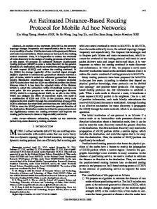
in terms of power and network utilization than the incremental cost of transmitting a few more bytes, we do not use this overhead metric. B.2 Transient state behavior This is the case where 10 new connections are initiated every 60 seconds for the first 300 seconds of simulation. This set of simulations do not have any warmup period. Figure 4 gives the packet latencies, packet delivery rates and throughputs for the 50-node network. ADV gives 70% lower latency than AODV and 50% lower than DSR for the first five intervals because of the connection-initiation process carried out at the start of any new connection. Furthermore, ADV latencies remain stable after 300 seconds (no new connections initiated after this time), while those of AODV and DSR increase, indicating that it stabilizes faster than the two on-demand algorithms. Packet delivery rates and throughputs are almost the same, and better than those of DSR, for AODV and ADV.

IEEE INFOCOM 2001

9

450

40 connections, 20 m/s MAC layer level overhead (pkts/s)

IP layer Routing Overhead (pkts/s)

40 connections, 20 m/s adv aodv dsr

400 350 300 250 200 150 100 50 0 0

20

40

60

80

3000 2500 2000 1500 1000

100

adv aodv dsr

500 0 0


20

40

60

80

100


Fig. 3. Routing overhead packets transmitted at IP and MAC layers of ADV, AODV and DSR for the high node mobility 50 node square field and 40 CBR connections case. 10-50 connections, 20 m/s

10-50 connections, 20 m/s adv 20 aodv dsr

70 60 50 40 30 20 adv aodv dsr

10 0 0

60

120

180

240

300

Simulation Time (sec)

80

Throughput (Kb/s)

Packets Delivery %


10-50 connections, 20 m/s

100

80

60 40 20

adv aodv dsr

0 360

420

0

60

120

180

240

300


15 10 5 0

360

420

0

60

120

180

240

300

360

420


Fig. 4. Average packet latencies, packet delivery rates and throughputs of ADV, AODV and DSR denoting the transient state conditions for the high mobility, 50-node square field.

Figure 5, gives the routing overhead. ADV transmits the least number of routing packets (which include initconnection and receiver-alert broadcasts). AODV performs the worst of all the three with its overhead 3 times more than ADV particularly after all the connections have been established. The MAC layer level overhead is as much as 50% lower for ADV. It is particularly noteworthy that ADV outperforms AODV and DSR in all relevant metrics for transient conditions, which should favor the ondemand algorithms. B.3 Steady-state performance in a 100-node network This section presents simulation results for a 100-node, rectangular field, high mobility network with 40 connections. Referring to Figure 6, ADV provides 50% less packet latencies than the two on-demand protocols and the packet delivery rates are also higher. ADV sustains higher loads and offers 30-90% higher loads over AODV

and DSR before saturation. Furthermore, ADV has the least overhead in packets/s. V. C ONCLUSIONS Proactive routing protocols tend to provide lower latency than on-demand protocols because they try to maintain routes to all the nodes in the network all the time. But the flip side for such protocols is the excessive routing overhead transmitted that is periodic in nature with out much consideration for the network mobility or load. Depending upon the periodicity interval, the dissemination of routing activity can become excessive (insufficient) at low (high) loads. To mitigate the effect of the periodic transmission of the updates, we have proposed some adaptive criteria that triggers routing updates based only on network load and mobility conditions. The overhead is reduced by varying the size and the frequency of the routing updates dynamically.

IEEE INFOCOM 2001

10

10-50 connections, 20 m/s

10-50 connections, 20 m/s MAC overhead packets (pkts/s)

adv aodv 300 dsr

Routing Overhead (pkts/s)

350

250 200 150 100 50

adv aodv dsr

1200 1000 800 600 400 200

0

0 0

60

120

180

240

300

360

420

0

60


120 180 240 300 360 420 Simulation Time (sec)

Fig. 5. Routing overhead at IP and MAC layer level of ADV, AODV and DSR (in packets/s) denoting the transient state conditions for the high mobility, 50 node square field. 40 connections, 20 m/s


150

100

50

0

adv aodv 250 dsr

80

Throughput (Kb/s)

adv aodv dsr

60 40 20

adv aodv dsr

0 0


100

Packets Delivery %


200

100

200

300

400

500

0


100

200

300

400

200 150 100 50 0

500

0

100


200

300

400

500


Fig. 6. Average packet latencies, delivery rates and throughputs of ADV, AODV and DSR for the high node mobility 100 node rectangular field and 40 CBR connections case. 40 connections, 20 m/s MAC layer level overhead (pkts/s)

IP layer Routing Overhead (pkts/s)

40 connections, 20 m/s 800

adv 700 aodv dsr 600 500 400 300 200 100 0 0

100

200

300

400

500


2500 2000 1500 1000 adv aodv dsr

500 0 0

100

200

300

400

500


Fig. 7. Routing overhead packets transmitted at IP and MAC layers of ADV, AODV and DSR for the high node mobility 100 node rectangular field and 40 CBR connections case.

We call this new proactive protocol with on-demand characteristics the Adaptive Distance Vector (ADV) protocol. We have shown using simulations that ADV outper-

forms on-demand protocols like AODV and DSR in many instances. The improvement is significant when the node mobility is high. ADV provides lower packet latencies

IEEE INFOCOM 2001

11

and sustains loads far beyond the saturating points of the on-demand protocols. Also ADV transmits the least number of routing packets at the IP layer, although because of its larger size of routing updates it transmits more routing bytes compared to AODV and DSR (However, in a wireless medium, obtaining the channel for transmission is much more expensive in terms of power and network utilization than transmitting a few extra bytes with each packet). Moreover, considering the actual number of routing packets transmitted on the physical layer, i.e. MAC layer level routing packets, ADV transmits the least number of packets, thus utilizing the channel more efficiently. AODV and DSR are not able to sustain high loads because of the large number of routing packets transmitted at MAC layer level. In AODV, the route request packets account for most of the routing packets. But in DSR, the large number of the unicast route reply and route error packets use considerable channel bandwidth in the form of RTS, CTS and ACK, that are control packets required for reliable transmission of unicast packets. The good performance of the ADV in the transient conditions of a network is noteworthy. The connectioninitiation process at the start of any new connection, which advertises the destination as an active receiver and enables quick initial route establishment, helps ADV adapt to sudden load changes quickly and thus, can be a good protocol in bursty traffic conditions. In summary, ADV is a strong candidate for the multihop, mobile, wireless environment. Since it combines both proactive and on-demand techniques, it exhibits the best characteristics of proactive algorithms and, at the same time, is responsive to the network needs and conditions. In future, we would like to study the performance of ADV and the on-demand protocols for real-time traffic. With ADV providing lower latencies it should be a more suitable protocol for real-time traffic scenarios. It will be also interesting to investigate the effect of ADV and the on-demand protocols on TCP performance. As routes are frequently refreshed using updates in ADV, it helps maintain route connectivity all the time as required in TCP. R EFERENCES [1] J. Broch et al., “ A performance comparison of multi-hop wireless ad hoc network routing protocols” in ACM Mobicom ’98, Oct. 1998. [2] CMU Monarch Group, “CMU Monarch extensions to the NS-2 simulator.” Available from http://monarch.cs.cmu.edu/cmuns.html, 1998. [3] K. Fall and K. Varadhan, “NS notes and documentation.” The VINT Project, UC Berkeley, LBL, USC/ISI, and Xerox PARC. Available from http://www-mash.cs.berkeley.edu/ns, Nov. 1997. [4] IEEE Computer Society LAN/MAN Standards Committee, “Wireless LAN medium access control (MAC) and physical layer (PHY)

specifications.” IEEE Std. 802.11-1997. IEEE, New York, NY 1997. [5] S. R. Das, C. E. Perkins, and E. M. Royer, “Performance comparison of two on-demand routing protocols for ad hoc networks,” in IEEE Infocom 2000, Mar. 2000. [6] D. B. Johnson et al., “The dynamic source routing protocol for mobile adhoc networks.” IETF Internet Draft. http://www.ietf.org/internet-drafts/draft-ietf-manet-dsr-02.txt, 1999. [7] C. E. Perkins, E. M. Royer, and S. R. Das, “Ad hoc on demand distance vector routing.” IETF Internet Draft. http://www.ietf.org/internet-drafts/draft-ietf-manet-aodv-03.txt, 1999. [8] S.Lee, Mario Gerla, and C.K.Toh, “A simulation study of tabledriven and on-demand routing protocols for mobile ad hoc networks,” in IEEE Network Magazine, Aug. 1999. [9] E.Royer, and C.K.Toh, “A review of current routing protocols for ad hoc mobile wireless networks,” in IEEE Personal Communications Magazine, pp.46-55, Apr. 1999. [10] C. Cheng, R. Riley, and S. P. R. Kumar, “A loop-free extended Bellman-Ford routing protocol without bouncing effect,” in ACM SIGCOMM ’89, pp. 224–236, 1989. [11] P. Johansson et al., “Scenario-based performance analysis of routing protocols for mobile ad-hoc networks,” in ACM Mobicom ’99, Aug. 1999. [12] R.V.Boppana, M.K.Marina and S.P.Konduru, “An Analysis of Routing Techniques for Mobile and Ad Hoc Networks”, in High Performance Computing ’99, Dec. 1999. [13] D. E. Comer, ed., Internetworking with TCP/IP: volume 1. Prentice Hall, Inc., 1995. [14] V. D. Park and S. Corson, “A highly adaptive distributed routing algorithm for mobile wireless networks,” in IEEE INFOCOM ’97, pp. 1405–1413, Apr. 1997. [15] C. Hedrick, “Routing information protocol.” RFC 1058, 1988. [16] P.Jacquet et al., “Optimized Link State Routing protocol (OLSR).” IETF Internet Draft. http://www.ietf.org/internetdrafts/draft-ietf-manet-olsr-01.txt, 2000. [17] R.E.Bellman, Dynamic Programming. Princeton: Princeton Univ. Press, 1957. [18] Z. J. Haas and M. R. Pearlman, “The zone routing protocol (ZRP) for ad hoc networks.” IETF Internet Draft. http://www.ietf.org/internet-drafts/draft-ietf-manet-zone-zrp00.txt, 1997. [19] M. Jiang, J. Li, and Y. C. Tay, “The cluster based routing protocol (CBRP) for ad hoc networks.” IETF Internet Draft. http://www.ietf.org/internet-drafts/draft-ietf-manetcbrp-spec-01.txt, 1999. [20] R. Sivakumar et al., ” CEDAR: Core Extraction Distributed Ad hoc Routing ,” in IEEE Journal on Selected Areas in Communication, Special Issue on Ad hoc Networks, Vol 17, No. 8, 1999. [21] C. Toh, “Associativity based routing protocol (ABR) for ad hoc networks.” IETF Internet Draft. http://www.ietf.org/internet-drafts/ draft-ietf-manet-longlived-adhoc-routing 00.txt, 1999. [22] C. E. Perins and P. Bhagwat, “Highly dynamic destinationsequenced distance vector (DSDV) for mobile computers,” in ACM SIGCOMM ’94, pp. 234–244, Aug. 1994. [23] B. Tuch, “Development of WaveLAN, and ISM band wireless LAN,” AT&T Technical Journal, vol. 72, pp. 27–33, July 1993.