Graduate School of Industrial Administration, CMU, Pittsburgh, PA 15213. ... in the automotive parts supply industry as well as in the laminate industry (that ...
An Algebraic Geometry Algorithm for Scheduling in Presence of Setups and Correlated Demands Rekha R. Thomas Sridhar R. Tayur Cornell University y Carnegie Mellon University� N. R. Natraj Carnegie Mellon Universityz December 1992; Revised June 1994
Abstract
We study here a problem of scheduling n job types on m parallel machines, when setups are required and the demands for the products are correlated random variables. We model this problem as a chance constrained integer program. Methods of solution currently available { in integer programming and stochastic programming { are not su�cient to solve this model exactly. We develop and introduce here a new approach, based on a geometric interpretation of some recent results in Grobner basis theory, to provide a solution method applicable to a general class of chance constrained integer programming problems. Our algorithm is conceptually simple and easy to implement. Starting from a (possibly) infeasible solution, we move from one lattice point to another in a monotone manner regularly querying a membership oracle for feasibility until the optimal solution is found. We illustrate this methodology by solving a problem based on a real system. Key Words: Scheduling, Chance Constrained Programming, Integer Programming, Decomposition, Grobner Basis, Polynomial Ideals.
1 Introduction Firms are becoming increasingly aware that e�ective management of capacity constrained resources on the shop oor is essential to remain pro table in the presence of inherent variability of the marketplace. There are many instances, especially in the plants of industrial suppliers, where a set of jobs whose demands are random and correlated have to be scheduled on a bank of machines, not necessarily identical, with a minimum loss of capacity and � Graduate School of Industrial Administration, CMU, Pittsburgh, PA 15213. y School of Operations Research and Industrial Engineering, Cornell University, Ithaca, NY 14853. z Graduate School of Industrial Administration, CMU, Pittsburgh, PA 15213.
1
minimum costs due to setups while meeting a high level of service. This is especially typical in the automotive parts supply industry as well as in the laminate industry (that supplies to Printed Circuit Board manufacturers), where a large group of suppliers compete on price and service. The literature has recorded many models that consider the setup issues in presence of known demand. Several approaches dealing with these hard problems have resulted in implementable algorithms. In many cases, these results are applicable to situations with low variability of demand and low correlation between job types. However, these results are not transferable to a scenario where the job types that have low setup times or costs on a particular machine can have a strong positive correlation in demand because of their similarity in features. If these jobs are scheduled on the same machine based solely on setup cost information and mean demand values, the positive correlation in demand between products may result in poor service as the capacity of the machine on which they are scheduled constrains a quick response. Similarly, scheduling two job types with negative correlation of demand on the same machine is preferable from a demand management point of view; however, the setup costs and times involved may be high. While the variability of demand can be reduced by managing the customer ordering process appropriately (for example, by negotiating a contract for pre-committing a certain xed amount every period), the correlation structure usually cannot be a�ected by supplier rms as the correlations arise due to inherent end-product features, and so this is a problem that cannot be resolved by negotiations with customers. Consider the following scenario with three product types and two machines to illustrate the situation. Let products A, B and E with (random) demands DA , DB and DE (in any period) have means D^ A , D^ B and D^ E . Let machines � and have capacities C� and C respectively. Let the setup times for the products be Sij , and the setup costs be Kij for i = A; B; E and j = �; . Let the processing times per unit be 1 on both machines for all product types. Suppose products A and B are scheduled on machine � and product E is scheduled on machine . From a deterministic point of view, the cost in any period is KA� + KB� + KE . This schedule is an optimal solution to a deterministic problem of minimizing setup costs if, for example, KA� < KA ; KB� < KB ; KE� > KE and D^ A + D^ B � C� ? SA� ? SB�; D^ E � C ? SE . From a stochastic viewpoint, however, there is a possibility that demands will exceed the allotted production capacity in any 2
period, resulting in a shortfall. When this happens, (1) the excess demand is backlogged (and so incur penalty costs), or (2) the excess demand is satis ed from inventory which in turn needs to be replenished (and so incur inventory costs), 1 or (3) the excess demand is lost (and so lose the margin and possibly market share) or (4) overtime is required to make up the shortfall (and so pay overtime costs). The point is, in all cases, there are costs incurred due to exceeding the capacity in any period, and regardless of the speci c remedial strategy the rm chooses, there is reason to schedule jobs on machines to avoid frequent occurences of a shortfall. In the schedule discussed above, the shortfall probability is (1-ProbabilityfDA + DB � C� ? SA� ? SB�; DE � C ? SE g). This value of shortfall probability may be higher than the rm nds reasonable. A di�erent schedule may satisfy the maximum allowable shortfall probability but may cost more in setups. The trade-o� for the rm, therefore, is between shortfall management required due to demand correlation (and variance) and costs incurred due to setups. Rather than prescribe an optimal value for , the probability of no shortfall, we will provide the optimal scheduling of jobs to machines for every . This is because, a value of that a rm selects depends on the strategy and costs of making up (or losing) excess demand. It should be noted that the e�ects of correlation and variation in presence of capacity constraints and multiple items on performance characterstics can be often nonintuitive. In spite of this, many crucial capacity allocation and scheduling decisions on the shop oor are made without a sound scienti c analysis. Often one relies on intuition or approximate extensions of deterministic models due to the lack of appropriate models and solution methods to tackle problems of this type. It is this void that we attempt to ll in this paper by developing a model and a solution methodology that are broadly applicable. Our model formulation and the overall solution method is presented in detail in Section 2. Our formulation provides an increased exibity in scheduling by allowing lot splitting. The total demand of a particular job type, if necessary, is split into pieces (or lots), and each lot is scheduled on a di�erent machine. In an uncapacitated setting, there would be no incentive to split into lots i.e., every job type would be made on a particular machine and the solution is straightforward (Section 2.3). However, the presence of capacity constraints and the desire to lower the frequency of shortfall occurences make it bene cial to allocate capacity on several machines for a given product type. 1 In a dynamic in nite horizon capacitated model it can be shown that the amount of inventory (as safety
stock) required depends on the shortfall distribution. Our model here should not be considered as static.
3
The solution to our problem of scheduling in the presence of setups and correlated demands, therefore, is the set of optimal solutions to a sequence of chance constrained integer programs, each at a di�erent level . We show that the set of optimal schedules for di�erent
are level sets; a particular schedule remains optimal for an interval of values of . Our solution method di�ers signi cantly from available techniques. Indeed, impressive advances in stochastic programming { in particular chance constrained programming with continuous variables and normal demands { have helped in solving many practical problems that have been formulated as convex programs with chance constraints (Wets [12]). However, while these methods have been successful without the integrality constraint, no satisfactory solution method exists for models that have integer variables and non-separable chance (probabilistic) constraints arising from non-normal distributions. In our setting, (1) the probabilistic constraint is not separable, (2) with only a handful of large customers ordering in batches, the normality assumption on demand may be violated signi cantly and (3) integer variables are required to model setup decisions. A subsequent section reviews some of the available techniques. The main technical contribution of this paper is to provide a novel method to solve this class of problems. Our formulation is an instance of the following general problem, whose constraints can be separated into four categories: (P0)
minimize
Pn c x i i i =1
subject to: P (C1) ni=1 aij xi � bj j = 1; : : :; m1 P (C2) ni=1 aij xi � bj j = m1 + 1; : : :; m1 + m2 (C3) (x1 ; : : :; xn) 2 S (C4) xi 2 N i = 1; : : :; n; where S is a set in Nn , and whether or not any (x1 ; : : :; xn ) belongs to S can be veri ed e�ciently by a membership oracle. Note that S will depend on . Without constraint (C3), the problem is an integer program (IP). While constraints (C1) and (C2) look similar, the IP is easily solvable without the complicating constraints (C2). Furthermore, the structure of the constraints (C2) is similar to the constraints that de ne S . This structure lends itself to a decomposition that separates the constraints (C1) from (C2), and stores constraints (C2) 4
by expanding the (available) membership oracle for (C3). We refer to the integer program obtained by removing constraints (C2) and (C3) from (P0) as the reduced IP. The solution method for (P0) rst obtains an optimal solution of the reduced IP. If this is infeasible for (P0), we walk to other solutions of the reduced IP by moving along certain speci ed directions, querying the membership oracle each time to check feasibility with respect to (P0). We discuss this in detail shortly. An essential component of our solution technique, therefore, is to nd an appropriate set of directions which can be used to walk in a systematic manner from the optimal solution of the reduced IP to other solutions. These directions arise from a geometric interpretation of an algebraic algorithm to solve integer programs problems due to Conti and Traverso [2]. This algebraic algorithm uses the theory of Grobner basis of polynomial ideals to solve integer programs. Starting at an integer point (infeasible for (P0)), the algorithm traces a path to the optimal solution of (P0) using only those directions speci ed by the associated Grobner basis. In our case the integer program in question is the reduced IP whose optimal solution can be found quickly due to special structure of the problem. The elements of the Grobner basis given by the Conti-Traverso algorithm can be interpreted geometrically as a set of directions 2 that can be used to trace paths from every non-optimal solution to an integer program to the optimal solution. Therefore, we can walk back from the optimal solution to every other feasible solution of the integer program by simply reversing these paths. Our algorithm terminates when all paths (starting from the optimal point of the reduced IP) are pruned. A path can be pruned in three ways: (1) it enters the feasible region of (P0) (satis es the expanded membership oracle); (2) it lands on a point that violates the non-negativity constraint; and (3) it lands on a point (still infeasible for (P0)) whose cost is higher than the best feasible solution found so far. A straightforward comparison of costs of points that are at the leaves of the paths that have entered the feasible region provides the optimum. If all the paths have been pruned and no feasible solution has been found, then the problem is infeasible. To guarantee that this method always terminates at the optimum for (P0) or nds the problem infeasible (starting from the optimum for the reduced IP), we need to prove the following. One, reversing the directions and walking from the reduced IP optimum using these (reversed) directions always lands on a point that is feasible for the reduced IP if non2 More general results on Grobner basis methods for integer programming appear in Thomas [11]. We
use here only a few results relevant to our problem.
5
negativity constraints are satis ed. Two, all feasible points of the problem can be reached using only these directions. Three, on every path, every step deeper into the polytope (starting from the reduced IP optimum) increases the cost monotonely. We show that all the above are indeed true. The solution method outlined above is especially appropriate to the model we formulate for the following additional reasons. The Grobner basis does not depend on the right hand side of the IP constraints but only on the costs and the constraint matrix. In our formulation, the right hand side can be varied based on management judgement on lot splitting. Furthermore, as we vary , we need to solve a nested set of integer programs with chance constraints, and the expanded membership oracle (which stores the probabilistic constraint as well as the complicating constraints) can be designed in such a way that all these nested problems are solved without solving for the Grobner directions each time. In the past, a general pessimism on the usefulness of Grobner basis algorithms has arisen from the fact that the number of basis elements can be very large and the computational time to obtain these elements can be prohibitive. As will become clear in Section 3, we need a set of starting generators to compute the Grobner basis. Indeed, a naive application of available methods to choose the starting generators makes the approach computationally infeasible. However, we show that our formulation has su�cient special structure that enables us to provide a set of starting generators that nd the Grobner basis elements quickly. The rest of this paper is organized as follows. Section 2 presents the model, the overview of the solution procedure and a critique of available methods. In Section 3, we provide a geometric algorithm based on recent results in Grobner basis theory, derive a good set of starting generators and provide an example to illustrate the overall procedure. In Section 4, we construct an e�cient membership oracle and solve a problem based on a real system. Section 5 discusses another possible application of this methodology and concludes this paper. 6
2 The Model 2.1 Formulation Formally, the problem is to schedule n job types (indexed by i), whose demand in any given period is a random vector (D1; : : :; Dn), on m machines (indexed by j ) that have a capacity of Cj , j = 1; : : :; m. The probability distribution of demand of the n job types in any period is F (x1 ; : : :; xn) = ProbabilityfD1 � x1 ; : : :; Dn � xn g, with means (D^ 1; : : :; D^n ). The setup time for job type i on machine j is Sij . Let Kij denote the setup cost for job type i on machine j . To facilitate lot splitting, we have Mi ; i = 1; : : :; n, a set of management speci ed integers, that limits the maximum pieces (or lots) the demand of job type i can be partitioned into. Thus, if M1 = 4, then on any machine only multiples of 41 of the demand for product type 1 can be produced. Let L0ij be the cost of producing a unit of product type i on machine j , and de ne Lij = MD^ ii L0ij . The processing time for a unit of job type i on machine j is pij . Let be the probability of no shortfall. The problem is modeled as the following chance constrained program: (P1)
minimize subject to:
P P (K z + L y ) ij ij i j ij ij Pm y = M 8i (1) ij i j Mizij � yij 8i; j (2) Pn p D y + Pn S z � C 8j (3) ij ij j i ij M ij i P P Probf n p D y + n S z � C 8j g � (4) =1
^i
=1
i
i i=1 ij Mi ij
=1
i=1 ij ij
j
zij 2 f0; 1g; yij 2 f0; 1; : : :; Mig
(5)
Variable zij equals 1 if job type i is scheduled on machine j ; otherwise it is set to zero. Variable yij , an integer between zero and Mi , represents how many multiples of M1i of demand of product i are scheduled on machine j . Thus, if in a period the demand yij D will be scheduled on machine j . In our setting, therefore, realized for product i is Di , M i i allocation of capacity and scheduling go hand in hand. The objective is to minimize the expected costs due to setups and production. Equation (1) states that all of the demand for product i needs to be scheduled. Equation (2) states that production for job type i cannot take place on machine j unless the appropriate setup 7
has occured. Equation (3) states that the average demand allocated to a machine does not exceed its capacity. These are the complicating constraints of (P1). Equation (4), the probabilistic constraint, states that the probability of production time and setup time not exceeding the capacities on the respective machines is at least . Notice the similarity in structure between constraint (3) and constraint (4). In the framework of problem (P0), equations (1)-(2) constitute the set (C1), equation (3) is the set (C2), equation (4) corresponds to (C3) and equation (5) corresponds to (C4). Thus, the reduced IP consists of constraints (1), (2) and (5) only. Note that doubling Mi provides more exibility in scheduling due to more choices of lot-splitting. However, if Mi and Mi0 are relatively prime with Mi < Mi0 , it is possible that there is a feasible schedule with Mi but not with Mi0. To avoid computing the Grobner basis several times when some Mi is varied (in a study of the e�ect of Mi on costs) we can de ne M � maxi=1;:::;n Mi , over all possible candidates for Mi that we are interested in. In equation (2), we can replace Mi by M . This assures that the constraint matrix of the reduced IP does not vary.
2.2 Overview of Solution Method Our solution method separates constraints (1)-(2) and (5) from (3)-(4). The motivation for this decomposition is the fact that the reduced IP is trivial to solve, while adding constraint (3) to it makes the problem NP-Complete (recall the knapsack problem). The similarity in structure between (3) and (4) makes it especially attractive to move constraint (3) into the membership oracle. Samples from the demand distribution are appropriately stored to make up the membership oracle. In case we do not have an empirical distribution, we can obtain a desired accuracy for the probabilistic constraint at level by selecting an appropriate number of samples from F (x1 ; : : :; xn ) (Hoe�ding [5]). It will be shown that a further decompostion of the reduced IP (by jobs) is possible. This will imply that the elements of the Grobner basis for the reduced IP can be obtained by concatenation of n (smaller) Grobner bases, one basis for each job type { a major computational advantage. This will be discussed in detail in Section 3.3. Let (yijr ; zijr ) be the optimal solution to the reduced IP (superscript r corresponds to `reduced'). Starting from this point, if infeasible for (3)-(4), we use the Grobner directions and walk on the lattice. At each step, we query the membership oracle. When all paths 8
are pruned, we can obtain the required optimal solution by a straight-forward comparison of active feasible points, or claim that the problem is infeasible.
2.3 The Reduced IP Recall that the reduced IP consists of constraints (1)-(2) and (5). This problem decomposes easily by product types. The optimal solution can be obtained by rst observing that because of linear costs of production, a xed charge for setup and no capacity constraint, there is no reason to split lots. Thus, for each job type, we simply nd the machine on which this job type can be produced in the cheapest manner and call it i (in case there is a tie, we pick the lowest index). Thus (for each i), (Ki i + Mi Li i ) � (Kij + Mi Lij ) 8j , and i is the smallest j for which this is true. The optimal solution to the reduced IP is obtained by setting zi r i = 1, yi r i = Mi and the rest of the variables to zero. If this satis es the complicating constraints (equation (3)) as well as the probabilistic constraint (equation (4)), then it is the optimal solution to (P1).
2.4 Review of Existing Solution Methods As stated in the introduction, the results of deterministic scheduling models do not carry over to our situation. More importantly, the techniques commonly used in stochastic programming also fail in our setting. Recall that our probabilistic constraint is of the form P fHx � hg � , with a random matrix H and integer variables x. We brie y review four available methods for solving chance constrained programming problems and point out their inapplicability here. See Wets [12] for details and references for the descriptions below. Consider rst the approach, useful for problems with continuous variables, that constructs a deterministic equivalent. This converts the problem into a convex non-linear programming problem which can be solved by gradient methods. Our problem may not have a deterministic equivalent of the type usually studied by stochastic programmers. This is because we have a joint constraint, rather than a constraint for each j = 1; : : :; m and the demands typically arise from a distribution other than the multi-variate normal. A second method, a dual approach to solve continuous variable problems in presence of joint chance constraints, requires the coe�cient matrix in the chance constraint to be deterministic. In our formulation, however, the coe�cient matrix in the probabilistic constraint is random. It has been shown that when this coe�cient matrix is random, the set 9
of feasible solutions that satisfy the probabilistic constraint is non-convex in general, thus precluding the use of convex optimization techniques. A third approach, based on outer approximations for mixed integer non-linear problems has been successfully applied for problems arising in chemical engineering. This method, however, requires a deterministic equivalent, convexity of the feasible region, as well as an explicit function that can be di�erentiated. These conditions are not satis ed by the problem at hand. See Duran and Grossmann [4] for details of this method. A fourth approach, based on recent results on rapidly mixing Markov chains, nds a near optimal solution for a certain class of chance constrained programs (with continuous variables) using a randomized algorithm. See Kannan et. al [6] for details. To summarize, although many available methods can be adapted to heuristically solve complex integer non-linear problems that may arise from chance constrained models, no particular one solves our problem exactly. Ultimately, we believe that all these approaches should form part of a tool kit for analyzing complex problems modeled in this fashion.
3 Solution Method 3.1 The Walk-Back Procedure In this section we describe a systematic procedure to walk from the optimum of an integer program to any other feasible lattice point in its feasible region. Given a feasible lattice point �, the path to this point from the optimum is obtained by moving from one feasible solution to another according to certain rules. The objective function value of successive lattice points in this path increases monotonically. In Section 2.3 we showed that the optimal solution of the reduced IP was easy to nd but that it may be infeasible with respect to the constraints in the expanded membership oracle. Since every feasible solution of the overall problem (P1) is also feasible for the reduced IP, we can use the above mentioned paths to walk from the optimum of the reduced IP, to feasible solutions of (P1). We give an algorithm that uses these paths to nd a su�cient set of feasible solutions to (P1), from which the optimal solution can be identi ed easily. Consider an integer program of the form: 10
Min cx subject to Ax = b
x 2 Nn where A 2 2 and c 2 Rn . Let IP denote all integer programs of the above form, obtained by varying the right hand side vector b but keeping A and c xed. Let IP(b) denote that integer program from the above family with right hand side vector b. We assume that each IP(b) is bounded with respect to the cost function c. Consider the map � : Nn 7! Zm such that � (x) = Ax. Given a vector b 2 Zm , the set of feasible solutions to IP(b) constitute � ?1(b), the pre-image of b under this map. We identify � ?1 (b) with its convex hull and call it the b ? fiber of IP. Therefore the b- ber of IP is just the convex hull of all feasible solutions to IP(b).
Zm�n ; b
Zm
De nition 1 We call > a term order on Nn if > has the following properties: (1) > is a total order on Nn , (2) � > ) � + ! > + ! for all �; ; ! 2 Nn (i.e., > is compatible with sums), (3) � > 0 for all � 2 Nn nf0g (i.e., 0 is the minimum element). Each point in Nn is a feasible solution in some ber of IP - i.e., � in Nn is a feasible solution in the A� - ber of IP. Suppose we now group points in Nn according to increasing cost value cx. Since more than one lattice point can have the same cost value, this ordering is not a total order on Nn . We can, however, re ne this to create a total order by adopting some term order >, to break ties among points with the same cost value. Let >c denote this composite total order on Nn that rst compares two points by the cost c and breaks ties according to >. We may think of >c as a re nement of the cost function c. It can be checked that >c satis es properties (1) and (2) of De nition 1. However, >c may not satisfy (3) and therefore, >c is not always a term order on Nn . Example : Consider 9 N2 and c = (?1; 2). c:(0; 0) = 0 = ) (0; 0) >c (1; 0): c:(1; 0) = ?1 ; We now replace the objective function of programs in IP by its re nement >c . This change does not a�ect the optimal value of a member of IP, but since >c is a total order on Nn it insures a unique optimum in every ber of IP. Let S denote the set of all points in Nn that are non-optimal with respect to >c in the various bers of IP. The following lemma characterizes the structure of S . 11
Lemma 1 There exists a unique, minimal, nite set of vectors �(1); : : :; �(s) 2 Nn such that the set of all non-optimal points with respect to >c in all bers of IP is a subset of Nn of the form
S = Ssi (�(i) + Nn ). =1
Proof: First we show that if � 2 S , then � + Nn � S . This will imply that S is an order ideal. If � 2 S , then � is a non-optimal point with respect to >c in � ?1(A�). Let be the unique optimum in this ber with respect to >c . Consider � + ! , + ! for ! 2 Nn . Then 1. A(� + ! ) = A( + ! ) since A� = A . 2. (� + ! ); ( + ! ) 2 Nn since �; ; ! 2 Nn . 3. � >c ) � + ! >c + ! . (1) - (3) implies that � + ! is not the optimal lattice point in the ber � ?1(A(� + ! )). Therefore � + ! 2 S . Since ! is an arbitrary element in Nn , this establishes that � + Nn � S . By Dickson's Lemma, every order ideal in Nn has nitely many minimal elements. Applying this to S , we conclude that there exists a unique minimal set of points �(1); :::; �(s) 2 S such that
S = Ssi (�(i) + Nn):2 =1
We now de ne a test set for IP dependent on the matrix A and a re ned objective function >� . 3
De nition 2 A set G>� � Zn is a test set for the family of integer programs IP (with
respect to the matrix A and re ned cost function >� ) if (I) for each non-optimal point � in each ber of IP, there exists g 2 G>� such that � ? g is a feasible solution in this ber and � >� � ? g and (II) for the optimal point in a ber of IP, ? g is infeasible for every g 2 G>� .
A test set for IP gives an obvious algorithm to solve an integer program in IP provided we know a feasible solution to this program. At every step of this algorithm, there either exists an element in the test set which when subtracted from the current solution yields an improved solution, or there will not exist such an element in the set. In the former case the solution at hand is non-optimal whereas in the latter case it is optimal. If a new solution is obtained, we repeat until the process stops at the unique optimum of the ber. Since 3 See Scarf [7] for a di�erent test set.
12
each integer program considered is bounded with respect to the objective function >c , the procedure is guaranteed to be nite. We construct a set G>c for IP as follows. Let G>c = fgi = (�(i) ? (i)); i = 1; :::; sg, where �(1); :::; �(s) are the unique minimal elements of S and (i) is the unique optimum with respect to >c in the A�(i) - ber of IP. We show below that G>c is indeed a test set for IP and in the next subsection we prescribe an algorithm that computes G>c without explicitly determining �(i) and (i). Notice that (�(i) ? (i)) is a lattice point in the subspace S = fx 2 Zn : Ax = 0g. Geometrically we can think of (�(i) ? (i)) as the
-
directed line segment g~i =[�(i); (i)] in the A�(i)- ber of IP. The vector is directed from the non-optimal point �(i) to the optimal point (i) due to the minimization requirement in the problem.
Observation 1 Adding a vector v 2 Nn to both end points of g~i translates g~i from the A�(i)- ber of IP to the A(�(i) + v) ber of IP.
We now consider an arbitrary ber of IP and a feasible lattice point � in this ber. For each vector g~i in G>c , check if it can be translated through some vector v in Nn such that the tail of the translated vector is incident at � . At � draw all such possible translations of vectors from G>c . Notice that the head of a translated vector is also incident at a feasible lattice point in the same ber as � . We do this construction for all feasible lattice points in all bers of IP. From Lemma 1 and the de nition of G>c , it follows that no vector in G>c can be translated by v 2 Nn such that its tail meets the optimum on a ber. We now state the main result of this section.
Theorem 1 The above construction builds a connected, directed graph in every ber of IP.
The nodes of the graph are all the lattice points in the ber and the edges are the translations of elements of G>c by non-negative integral vectors. The graph in a ber has a unique sink at the opimum in the ber with respect to >c and the outdegree of every non-optimal lattice point in the ber is at least one. Proof: Pick a ber of IP and at each feasible lattice point construct all possible translations of the vectors g~i from the set G>c as described earlier. This results in a possibly disconnected directed graph in this ber where nodes are the lattice points and edges the translations of elements in G>c . Let � be a non-optimal lattice point in this ber. By Lemma 1, � = �(i) + v for some i 2 f1; :::; sg and v 2 Nn . Now �0 = (i) + v also lies
13
in this ber and � >c �0 since �(i) >c (i). Therefore g~i translated by v 2 Nn is an edge in this graph and we can move along it from � to an improved point �0 in the same ber. This proves that from every non-optimal lattice point in the ber we can reach an improved point in the same ber by moving along an edge of the graph. The structure of S and the construction of the set G>c imply that the outdegree of the optimal solution is zero. Therefore, a directed path from a non-optimal point terminates precisely at the unique optimum of the ber. This in turn implies connectedness of the graph.2 We call the graph in the b- ber of IP the >c ?skeleton of that ber to denote the dependence of the graph on the re ned objective function >c . The following corollaries follow from Theorem 1.
Corollary 1 In the >c -skeleton of a ber, there exists a directed path from every non-
optimal point � to the unique optimum . The objective function value (with respect to c) of successive points in the path decreases monotonically from � to .
Corollary 2 The set G> is a uniquely de ned minimal test set for IP. Example 1 Consider the integer program: c
Minimize subject to
100a + 0b + 0c + 100d 2a + b + c + 3d = 30 a + c + 5d = 16 a; b; c; d non-negative and integer:
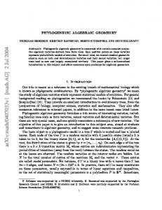
The feasible region of the integer program are the integer points in the (30,16)- ber. The extreme points are given by (a,b,c,d): (14, 0 , 2, 0 ), ( 0, 14, 16, 0), ( 0 , 20, 1, 3), (1, 19, 0, 3) and ( 11, 5, 0 , 1). To illustrate graphically, we draw the ber by projecting onto the b ? d co-ordinate plane (Figure 1). The extreme points on this plane are: (0,0), (14,0), (20,3), (19,3) and ( 5,1). All lattice points in the projection lift to become lattice points in the actual ber and viceversa. The test directions for this example are [(0; 2; 0; 1); (0; 0; 5; 0)] (direction P ) and [(1; 0; 0; 0); (0; 1; 1; 0)]
-
(direction Q). The (projections of) test directions in the b ? d plane are [(2; 1); (0; 0)] and
14
P
Q
(19,3) (20,3) (5,1) d (0,0)
(14,0) b
Figure 1: Projection on b-d plane for Example 1.
-
[(0; 0); (1; 0)], and (the projection of) the point (0,14,16,0), for example, is (14,0). Figure 1 also shows some paths (not the entire skeleton) from some feasible solutions (including all the extreme points) to the optimal solution using directions P and Q in the (30, 16)- ber. From point (0,14,16,0), we cannot travel to any other feasible point in the (30,16)- ber using directions P and Q; this is because direction P leads to (0,12,21,-1) and direction Q leads to (-1,13,15,0). This implies that (0,14,16,0) is the optimal solution. Consider the other extreme points. From (0,20,1,3) direction P leads to (0,18,6,2) and then to (0,16,11,1) and nally to (0,14,16,0). Direction Q, at all points in the path, leads to infeasible solutions (that violate non-negativity) and is therefore not used. From (11, 5, 0, 1), a repeated movement in direction Q (11 times) takes you to (0, 16, 11, 1). Now, direction P leads to (0, 14, 16, 0), the optimal solution. From (1, 19, 0, 3), direction Q moves you to (0, 20, 1, 3). Now, repeated application of direction P (3 times) leads you to (0, 14, 16,0). Finally, from (14, 0, 2,0), direction Q (14 times) leads to (0, 14, 16, 0). Note that from any non-optimal point, there may be several paths to the optimal solution in the (30, 16)- ber.
15
We are now ready to propose a solution method for problem (P1) from Section 2.1. Recall from Section 2.3 the reduced IP and its optimal solution. The feasible region of the reduced IP is given by constraints (1)-(2) and (5) of (P1). Consider the >c -skeleton of the appropriate ber. Suppose we now reverse the direction of all edges in this skeleton and call the resulting graph the reverse >c ?skeleton of the ber. Corollary 1 then implies that there exists a directed path P (�) in the reverse >c -skeleton of this ber, from the optimum of the reduced IP to the feasible lattice point � in the ber. Also, the objective function value of points reached as the path is traversed from to �, increases monotonically. We rst show that we can build the reverse >c -skeleton in a ber by reversing the orientations of vectors in the set G>c and repeating the construction described before Theorem 1. Let G>0 c denote the set of vectors in G>c with directions reversed. At a feasible lattice point � in a ber of IP, we draw all vectors from G>0 c that can be translated through some v 2 Nn such that its tail is incident at �. As before, the heads of the translated vectors are also incident at feasible lattice points in the same ber. Since only the orientation of the vectors in the test set was reversed, this construction and the previous one have the same underlying undirected graph in every ber. This proves the claim. We now use these paths in the reverse >c -skeleton of the reduced IP to nd a su�cient set of feasible solutions, Y , to (P1) from which the optimal solution to (P1) is obtained. Let be the optimum of the reduced IP and P (�) be a path in the reverse >c -skeleton of the ber from to �. Let P be a set of paths of the form P (�). We may assume that is infeasible for (P1) since otherwise we are done. Finding a Set of Feasible Solutions to (P1)
INITIALIZE : (i) P = fP ( )g, (ii) Y = �. REPEAT For P (�) 2 P , let P (!1 ); :::; P (!q) be the paths obtained by adding to P (�) those edges in G>0 c such that !i � 0. This insures that P (!i ) is a path in the reverse >c -skeleton. A path that leads to an infeasible point may be assumed to be pruned at �. FOR i FROM 1 TO q (i) IF !i feasible for (P1) let Y = Y [ f!i g and prune P (!i ) (feasibility is checked by querying the membership oracle) (ii) ELSE IF !i >c y for some y 2 Y then prune P (!i ) (the path if continued will give points that are more expensive 16
than those in Y ) (iii) ELSE P = fP [ P (!i )g. Delete P (�) from the set P . UNTIL all paths in P are pruned. Clearly all points in Y are feasible for (P1). Finiteness of the above procedure follows from the fact that the optimal solution to (P1) is bounded with respect to >c . Thus (P1) is infeasible if and only if Y is empty when the algorithm terminates. We now prove that the set Y contains an optimal solution to (P1).
Theorem 2 The points in Y with the least cost value c(y) are optimal for (P1). Proof: Let � be any feasible solution to (P1) and let y � 2 Y be a point with least cost c(y). Clearly � is feasible for the reduced IP and there exists a path P (�), in the reverse >c -skeleton, from the optimum of the reduced IP, to �. Note that P (�) may not be unique but any such path will su�ce for this proof. We identify P (�) with the sequence of nodes in the reverse >c -skeleton that constitute it, i.e., P (�) = f = u1 ; : : :; um = �g. Now let j 2 f1; : : :; mg be the largest number such that P (uj ) is in the set P of the above procedure at some stage. We have two cases to consider. (i) P (uj ) was pruned since uj became feasible for (P1): In this case, uj 2 Y and c(uj ) � c(y �). Also c(�) � c(uj ), since the successive nodes in P (�) have monotonically increasing cost when the path is traversed from to �. Therefore c(�) � c(y �). (ii) P (uj ) was pruned since uj >c y for some y 2 Y : Again, c(�) � c(uj ) � c(y �). Therefore, we have shown that in either case c(�) � c(y �) which proves the theorem.2
Using Theorem 2 we can identify the optimal solution to (P1) by a straightforward comparison of the costs of points in Y . We wish to emphasize that the solution method described for (P1) can be adapted in general for problems modeled in this way. Given an integer program in which some of the constraints are complicating and possibly non-linear, it is possible to create a reduced IP and a membership oracle and use the above solution method. The e�ciency of the procedure will depend heavily on how one separates the constraints into those that constitute the reduced IP and those that contribute to the membership oracle. 17
3.2 Computing Test Sets In this subsection we prescribe an algorithm to compute the test sets described in Section 3.1 by establishing the connections of these test sets with certain algebraic concepts. An important concept in the theory of polynomial ideals is that of a Grobner basis of an ideal (Buchberger [1]) with respect to a term order. These special bases can be computed using Buchberger's algorithm (Buchberger [1]) which has been implemented in most computer algebra packages. We show below that the test set G>c is equivalent to the reduced Grobner basis of a certain polynomial ideal with respect to the composite order >c . This immediately allows us to compute these test sets in practice, making the solution method proposed earlier, a feasible one. In order to establish the equivalence, we rst recall some basic de nitions and concepts (Cox et. al [3]) from the theory of polynomial ideals. Let k be any eld and let k[x1 ; : : :; xn] be the polynomial ring in n variables over k.
De nition 3 A subset I � k[x ; : : :; xn] is an ideal if it satis es: (i) 0 2 I (ii) If f; g 2 I , then f + g 2 I (iii) If f 2 I and h 2 k[x ; : : :; xn], then hf 2 I . 1
1
De nition 4 Let f ; : : :; fs be polynomials in k[x ; : : :; xn]. We say f ; : : :; fs is a basis P for I if I = < f ; : : :; fs > = f si hi fi : h ; : : :; hs 2 k[x ; : : :; xn]g. 1
1
1
=1
1
1
1
For ease of exposition, we let the monomial x�1 1 : : :x�n n be denoted by x� , where � 2 Nn . We may identify a monomial in k[x1 ; : : :; xn] with its exponent vector � 2 Nn . Recall from Section 3.1 the de nition of a term order on Nn . Under the above identi cation, > can be thought of as a term order on the monomials of k[x1 ; : : :; xn ]; that is, x� > x if and only if � > . This term order, therefore, identi es in every polynomial f 2 I , a unique initial term denoted in> (f ), which is the term of f involving the most expensive monomial with respect to >. We can now de ne the initial ideal of I with respect to >.
De nition 5 We call init> (I ) = < in> (f ) : f 2 I >, the initial ideal of I with respect to >.
Notice that init> (I ) is generated by monomials. 18
De nition 6 We say G> = fg ; : : :; gsg � I is a Grobner basis of I with respect to > if 1
init> (I ) = < in> (g1); : : :; in>(gs) > :
In other words, a Grobner basis of I is a special basis of I with the property that init> (I ) can be generated by the initial terms of the elements g1; : : :; gs in I . The condition on the initial terms of elements in G> does imply that G> is a basis of I . A Grobner basis of an ideal is not necessarily unique. We can however talk of the reduced Grobner basis of I with respect to > which is unique.
De nition 7 The reduced Grobner basis of I with respect to > is a Grobner basis G> of I such that: (i) in> (gi) has unit coe�cient for each gi 2 G> , (ii) For each gi 2 G> , no monomial of gi lies in < init> (G> ? gi ) >.
Given any basis of an ideal and a term order >, Buchberger's algorithm computes the reduced Grobner basis of the ideal with respect to this term order. We call the basis of the ideal needed as input to this algorithm, a starting basis. Conti and Traverso [2] describe an algebraic algorithm to solve integer programs using the theory of Grobner bases. We resort to their algorithm to obtain the ideal whose reduced Grobner basis corresponds to the test set G>c . Recall from Section 3.1 the family of integer programs IP with matrix A 2 Zm�n and cost function c. We denote the j th column of A by aj . Consider the map
' : k[x] = k[x1; : : :; xn] ? 7 ! k[ya1 ; : : :; ya ] xj ? 7 ! ya n
j
where y = (y1 ; : : :; ym ) and x = (x1 ; : : :; xn). Let J = kernel(') = ff 2 k[x] : '(f ) = 0g � k[x]. It may be checked that J is an ideal of k[x]. A binomial in k[x] is the di�erence of two monomials. We now recall a few facts about the ideal J .
Observation 2 Let �; be vectors in Nn . Then, the binomial x� ? x is in J if and only if A� = A where �; 2 Nn . Given an integral vector � 2 Zn , we can write it uniquely as � = �+ ?�? where �+ ; �? 2 Nn and have disjoint supports. 19
Lemma 2 (Sturmfels [10]) The ideal J is generated by binomials of the form fx�+ ? x�? : A� = 0; � 2 Zng. Recall the test set G>c = f(�(i) ? (i)); i = 1; : : :; sg, with respect to the composite order >c , which sorted points by cost c and then broke ties using a xed term order >. As in the identi cation of a monomial with its exponent vector, we identify the vector (�(i) ? (i)) with the binomial x�(i) ? x (i). For each gi in G>c , both �(i) and (i) were feasible solutions from the same ber of IP. This implies that A�(i) = A (i); �(i); (i) 2 Nn for all i = 1; :::; s. Therefore by Observation 2, < x�(i) ? x (i); i = 1; : : :; s >� J . Further, since �(i) >c (i) for all i = 1; : : :; s, we have that in>c (x�(i) ? x (i)) = x�(i) for all i. Therefore, < x�(i); i = 1; : : :; s >� init>c (J ). We now show that in fact we have equality here.
Theorem 3 The test set G> = fx� i ? x i ; i = 1; : : :; sg is the reduced Grobner basis of J with respect to >c .
c
( )
( )
Proof: We show that in>c (f ) is in the monomial ideal < x�(i); i = 1; : : :; s > for each polynomial f in J . By Observation 2 and Lemma 2, J = < x� ? x : A� = A ; �; 2 Nn >. We may assume that in> (x� ? x ) = x�. In fact the binomials of the above form form a universal Grobner basis for J and so it is enough to show that x� 2 < x�(i); i = 1; : : :; s > for each binomial x� ? x 2 J . Now in> (x� ? x ) = x� implies that � >c . Therefore � is a non-optimal point with respect to >c in the A�- ber of IP. Therefore � is in S , the S set of all non-optimal points from all bers of IP. By Lemma 1, S = si=1 (�(i) + Nn ). This implies that � = �(i) + v for some i 2 f1; : : :; sg and v 2 Nn . Therefore x�(i) divides x� which in turn implies that x� 2< x�(i); i = 1; : : :; s >. Therefore G>c is a Grobner basis for I with respect to >c . We now show that G>c is in fact the reduced Grobner basis of I with respect to >c . For x�(i) ? x (i) 2 G>c , we rst note that x�(i) 62< init>c (G>c ? gi) > since �(1); : : :; �(s) were a unique minimal set of generators for S . Also x (i) 62< init>c (G>c ? gi ) > since (i) was the unique optimum with respect to >c on its ber and so is not in S . Therefore G>c is the reduced Grobner basis for I with respect to >c . 2
In Section 3.1 we mentioned that >c is not always a term order on Nn . The Buchberger algorithm requires a term order as input for the calculation of Grobner bases to insure nite termination of the algorithm. Since >c may not always have 0 as the minimum element, 20
there is a danger of nding an in nite descending chain of monomials with respect to >c in the ideal J . In our case this is prevented by the fact that programs in IP are bounded with respect to cost and that the tie breaking term order is in fact a legitimate term order. Therefore >c can be used instead of a term order as the order in the Buchberger algorithm. In Section 4, we use the computer algebra package Macaulay (Stillman et. al [9]) to compute Grobner bases.
3.3 A Starting Basis In the previous subsection we showed that the test set G>c is equivalent, under certain identi cations, to the reduced Grobner basis of the ideal J with respect to >c . As mentioned before, we can use the Buchberger algorithm to compute this reduced Grobner basis of J . The Buchberger algorithm needs as input the order >c as well as a basis of J , which we call the starting basis. The order >c can be input to Macaulay by simply specifying the cost function c. Macaulay uses a default term order to break ties creating the composite order we require. A standard way to implicitly specify a basis of the ideal J associated with any integer program is given by the Conti-Traverso algorithm. This general approach was however seen to be rather infeasible from a computational point of view (see Section 4), except for small examples from the family of problems associated with the reduced IP from Section 2.3. We describe below the special starting basis we used to speed up calculations for the family of problems at hand. Recall the reduced IP from Section 2.3.
PP
(I) Minimize i j (Kij zij + Lij yij ) subject to: Pm y = M i j =1 ij
Mi zij � yij zij 2 f0; 1g; yij 2 f0; 1; : : :; Mig for all i; j
i = 1; : : :; n i = 1; : : :; n & j = 1; : : :; m
We convert this problem into the form of the general integer program in Section 3.1 by adding slack variables and forcing the the requirement that the variables zij have a value zero or one. The problem can be re-stated as: (II) Minimize
P P (K z + L y ) ij ij i j ij ij 21
(1) (2) (3)
such that:
Pm y ij j yij
= Mi +aij ?Mi zij =0 zij +bij = 1
i = 1; : : :; n i = 1; : : :; n & j = 1; : : :; m i = 1; : : :; n & j = 1; : : :; m
yij ;
aij ;
2N
i = 1; : : :; n & j = 1; : : :; m
=1
zij ;
bij
The matrix A, associated with this integer program can be divided into four blocks according to the four sets of variables yij ; aij ; zij and bij . Let I denote the identity matrix of size mn and 0 denote a matrix with all entries zero. Let D be the block diagonal (0; 1)coe�cient matrix associated with the constraints (1) of system (II). Let ?MI denote the coe�cient matrix of the variables zij , i = 1; : : :; n & j = 1; : : :; m in constraints (2) of system (II). We can then write A as the (n + 2mn) � (4mn) integer matrix :
2 3 D 0 0 0 6 7 A = 664 I I -MI 0 775 0 0
I
I
Let x = (y11; y12; : : :; ymn ; a11; : : :; amn ; z11; : : :; zmn ; b11; : : :; bmn). Consider the following set of binomials in k[x].
9 8 < yipaiq ? yiq aip; i = 1; : : :; n; 1 � p < q � m = G=: i = 1; : : :; n; j = 1; : : :; m ; bij ? aM ij zij ; i
By Observation 2, G is contained in J . We show below that G can be used as a starting basis of J by showing that G is in fact a Grobner basis of J . Let y denote the set of variables (y11; :::; ymn) and similarly a; z and b denote the other sets of variables. Then x = (y; a; z; b) and the underlying polynomial ring is k[x] = k[y; a; z; b]. Let > be a term order on k[x] such that b > y > z > a. Within a block, the variables are sorted lexicographically according to index.
Theorem 4 The set G is a Grobner basis for J with respect to the term order >. Proof: Notice rst that the initial term of every binomial in G with respect to > is the underlined term. It is enough to show that for every binomial x� ? x 2 J , with initial term x� , there is some g in G whose initial term divides x� . Observation 2 implies that x� ? x
22
is in J if and only if � ? 2 S = ft 2 Zn : At = 0g. We denote an element t in S by t = (ty ; ta ; tz ; tb ) to indicate the correspondence between components of t and the columns of A. We denote the components of ty by (Y11; :::; Ymn) and similarly for the others. We classify the elements in S in the following manner. (a) Let K1 = ft 2 S : ty = tb = 0g. Now t 2 K1 if and only if (ta ; tz ) 2 Z2mn belongs to the lattice S 0 = fw 2 Z2mn : A0 w = 0g where
2 3 -MI I 5 A0 = 4 0
I
But S 0 = f0g since A0 is an invertible square matrix. Therefore K1 = f0g. This implies that there is no binomial of the form x� ? x in J involving only the variables aij and zij . (b) Let K2 = ft 2 S : tb = 0g. Again t 2 K2 if and only if (ty ; ta ; tz ) 2 Z3mn belongs to the lattice S 00 = fw 2 Z3mn : A00w = 0g where
3 2 0 0 D 7 6 A00 = 664 I I -MI 775 0 0
I
By (a) above, we may assume that ty 6= 0. From the last mn rows of A00 we have that tz = 0. Therefore, t 2 K2 if and only if (ty ; ta) 2 S 000 = fw 2 Z2mn : A000w = 0g where
2 3 0 D 5 A000 = 4 I I
Let Yip be the left most non-zero component of ty . We may assume that Yip > 0 since S is the set of integer points in a vector space which implies that it contains the negative of every element in it. The ith row of D in A000 implies that there exists some q > p such that Yiq < 0. Therefore,
yip divides xt+ and yiq divides xt? . Consider now the last mn rows of A000. These rows imply that Aip = ?Yip < 0 and Aiq = ?Yiq > 0. Therefore,
yipaiq divides xt+ and yiq aip divides xt? . 23
The initial term of xt+ ? xt? with respect to > is xt+ since yip divides xt+ and yip is the most expensive variable among those present in this binomial. But this implies that the initial term of yip aiq ? yiq aip 2 G divides the initial term of xt+ ? xt? . Therefore, the initial term of all binomials associated with K2 is divisible by the initial term of an element in G. (c) Consider now a general element in S = ft 2 Zn : At = 0g with no variables restricted to be zero. By (a) and (b) above we may assume that tb 6= 0. Let Brs be the rst non-zero component of tb . As before, we may assume that Brs > 0. Therefore,
brs divides xt+ . But xt+ is the initial term of xt+ ? xt? under the term order being used, and this initial term is divisible by brs , which is the initial term of brs ? aM rsr zrs 2 G. Therefore init> (J ) =< in>(g); g 2 G > which proves that G is a Grobner basis of J with respect to the term order >. 2 The Buchberger algorithm is an iterative method that builds the Grobner basis in steps from a starting basis of the ideal and a term order >. At every step it tests if two members of the current partial Grobner basis can interact to give a new member whose initial term cannot be divided by the initial terms of all members currently present. If such a new member is generated, it is added to the current set of elements and the test continued until no new elements arise. The resulting set is a Grobner basis with respect to >. We now restate a criterion from Buchberger [1] which recognizes when two elements from the partial Grobner basis cannot interact to give a new element during the algorithm.
Lemma 3 (Buchberger [1]) If the initial terms of two polynomials f; g in the current
partial Grobner basis are relatively prime (i.e, have no common terms), then f and g cannot interact to generate a new element of the Grobner basis.
We now go back to the starting basis G we proposed and show that we can speed up the computation considerably by a decomposition idea along with an application of Lemma 3. Since G is a Grobner basis of J , it can be used as a starting basis for the Buchberger algorithm. We now draw attention to a special feature of this starting basis. We can group the elements of G according to job types in the following way. With job i we associate the set Gi consisting of all elements of G whose variables have i as its rst index. 24
S
9 8 < yipaiq ? yiq aip; 1 � p < q � m = Gi = : �G ; bij ? aM z j = 1 ; :::; m ij ij i
Therefore, G = ni=1 Gi . Consider the ideal Ji generated by the elements of Gi. Clearly Ji � J . We compute the reduced Grobner basis of Ji with respect to the same cost on the variables as before, by using Gi as the starting basis. Let GBi be the corresponding reduced Grobner basis. Notice that the elements of each Gi involve only a subset of the complete set of variables. Also two distinct sets Gi and Gj have no variables in common. We now compute the reduced Grobner basis for each such ideal Ji as i ranges over all the jobs. Let GB = Smi=1 GBi .
Corollary 3 The set GB = Smi GBi is the reduced Grobner basis G> of the ideal J . S GB is a basis of J since for each i, GB and G generate the Proof: Surely GB = m i i i i S m G was a basis of J . Suppose GB was the starting basis in same ideal J and G = =1
c
=1
i
i=1 i
the Buchberger algorithm used to compute the reduced Grobner basis of J with respect to the order >c . For each job type i, the reduced Grobner basis GBi already contains all new elements that came out of the interaction between two elements in Gi . We now prove that a binomial from the set GBi cannot interact with a binomial from a di�erent set GBj , to give a new element during the algorithm. Consider the ideal Ji associated with job i, its starting basis Gi and reduced Grobner basis GBi . Since GBi was obtained from Gi , its elements involve the same variables as those occuring in Gi . We now consider a di�erent job j and the associated reduced Grobner basis GBj . If f 2 GBi and g 2 GBj then they have no common variables since they came from Gi and Gj which had no common variables. In particular, the initial terms of f and g with respect to any term order are relatively prime. By Lemma 3, f and g cannot interact in the Buchberger process to give a new member of the nal Grobner basis. Therefore GB = G>c .2 The corollary above shows that we can decompose the starting basis according to jobs and compute the reduced Grobner basis of each piece separately and then concatenate these reduced Grobner bases to get the overall Grobner basis (test set) we are looking for. This decomposition results in tremendous increase in the speed of the computations involved. We believe that identi cation of problem speci c starting bases and its decomposition whenever possible should be a general strategy in solving large problems. In the next section we present some of our computational results as well as comparisons of this method with 25
the general Conti-Traverso algorithm for the speci c class of matrices associated with the reduced IP.
3.4 An Example In this section we illustrate the procedures described earlier using an example of scheduling a job on 2 machines. Thus m = 2 and n = 1. Let the production costs per unit be L011 = 3 and L012 = 4 and the setup cost per batch be K11 = 5 and K12 = 3. The machines are identical with a capacity of 10, the processing times and setup times are p11 = p12 = 1 and S11 = S12 = 1 respectively and M1 = 3. We are interested in nding the optimal schedule for = 0:6 using 100 samples of demand drawn from a normal distribution with a mean of 12 and a variance of 6. This instance corresponds to the following: 5z11 + 3z12 + 12y11 + 16y12
minimize such that:
y11 + y12 = 3 y11 ? 3z11 � 0 y12 ? 3z12 � 0 4y11 + z11 � 10 4y12 + z12 � 10 ProbfD1 y311 + z11 � 10; D1 y312 + z12 � 10g � 0:6 zij 2 f0; 1g; yij 2 f0; 1; 2; 3g
3.4.1 Grobner Directions In 8 dimensional space (y11; y12; a11; a12; z11; z12; b11; b12), the three elements of the starting basis for this problem as described in Section 3.3 are:
y11a12 ? y12a11, a311z11 ? b11, and a312z12 ? b12: 26
The six elements in the Grobner basis (test directions) obtained using Macaulay are:
1. 2. 3. 4. 5. 6.
y12a11 ? y11a12; 2 2 y12 b11 ? z11y11 a11a212; z12a312 ? b12; z12y12a212b11 ? z11y11a211b12; z11a311 ? b11; and z11y11a211a12 ? y12b11:
Note that y12 a11?y11 a12 is interpreted as the direction from (1; 0; 0; 1; 0; 0; 0; 0) to (0; 1; 1; 0; 0; 0; 0; 0).
3.4.2 Walk Back Procedure : An Illustration r = 3 and z r = 1 (other yij ; zij are The optimal solution to the reduced IP (Section 2.3) is y11 11 zero) with an objective function value of 41. This solution is not feasible for (P1) because it violates constraint (3).
Figure 2 illustrates the walk back procedure described in Section 3.1. Recall that constraints (3) and (4) are checked using a membership oracle; the details are described in Section 4.1. It should be noted that whenever we branch along a particular direction we also evaluate the nonnegativity of the variables in the new solution. If the solution violates nonnegativity constraints we prune the branch. (Thus we prune the branch along direction 1 from the reduced IP solution.) Otherwise, the membership oracle is queried for feasibility with respect to constraints (3) and (4). If the oracle returns a negative answer, we continue with the branching (as illustrated by branching along direction 3 from the reduced IP solution). If we obtain a feasible solution to (P1) the branch is pruned. In this example, from the reduced IP solution, we rst branch along direction 3 and then along direction 1. Since all the paths in Figure 2 have been pruned, the solution obtained is optimal. The oracle is set up in such a way so as to provide the highest for which this solution remains optimal; in this case it is 0:83. For higher values of we continue branching beyond depth 2. 27
Reduced IP solution : INFEASIBLE
y11 = 3; z11 = 1; Cost = 41 r
1
2
r
3 4 5
6
depth 1
2
1
3
4
5
6
depth 2
y11 = 2; z11 = 1 y12 = 1; z12 = 1 Cost = 48; = 0:83
Infeasible for (P1) Pruned due to violation of nonnegativity constraints
Feasible, OPTIMAL
Pruned due to feasibility for (P1)
Figure 2: Walk back procedure for the example.
4 Computational Experience 4.1 The Membership Oracle The membership oracle is constructed after the optimal solution to the reduced IP is found. Let �r = (yijr ; zijr ) be the optimal solution to the reduced IP (from Section 2.3). Whenever the empirical demands are available, we use them directly; otherwise, samples from the demand distribution are generated. The number of data points or samples, S , required depends on errors �1 ; �2 speci ed; see the next subsection for the exact relationship. Let (dk1 ; : : :; dkn ); k = 1; : : :; S , be the samples. The membership oracle is a table with m columns (one for each machine) and S + 1 rows (Rrpq ; p = 1; : : :; S + 1; q = 1; : : :; m). Each element in the rst S rows represents the slack in machine j for the sample corresponding P yiqr dp + zr S ), for p = to that row for the solution (yijr ; zijr ). Thus, Rrpq = Cq ? ni=1 ( M iq iq i i 1; : : :; S; q = 1; : : :; m. The (S + 1)st row stores the slack in the complicated constraint 28
P yiqr D^ + zr S ). Some of the elements in the table can be negative, of the IP, Cq ? ni=1 ( M i iq iq i implying that more than the available capacity has been used up for production and setups. Note that �r is feasible for problem (P1) if (S +1)st row elements of Rr are all non-negative, and there are at least S other rows of Rr that have all non-negative elements. If �r is not feasible for (P1), we walk onto other points using a walk back procedure. The walk back procedure is a variable depth procedure, starting from (yijr ; zijr ). The implementation requires: (1) a recursive call to a subroutine that moves one more step into the polyhedron in a test direction and (2) a three dimensional array (T ) that stores the change in each of the elements of Rr due to each test direction. Let a test direction be t gt = (yijt ; zijt ). Then Tpqt equals Pni=1 ( Myiqi dpi + ziqt Siq ) for p = 1; : : :; S ; q = 1; : : :; m and t TS+1qt = Pni=1 ( Myiqi D^ i + ziqt Siq ) for q = 1; : : :; m. At each call, the feasiblity of any point (�) is determined as follows. Let R� be a table for � analogous to Rr . We do not store this table but rather compute the table dynamically using Rr and T . A point � is feasible for problem (P1) if (S +1)st row elements of R� are all non-negative, and there are at least S other rows of R� that have all elements non-negative. To construct R�, let the path to � from �r be obtained by test directions (not necessarily P distinct) gt1 ; : : :; gtf . Then, R�pq = Rrpq + fi=1 Tpqi for p = 1; : : :S + 1; q = 1; : : :; m.
4.2 Number of Samples When the empirical data is not available, then we need to generate samples from the demand distribution, F (x1 ; : : :; xn) = ProbabilityfD1 � x1; : : :; Dn � xn g. We use the following result to determine the number of samples required.
Theorem 5 (Hoe�ding [5]) Let Sk = X + : : : + Xk , where the Xi are independent random variables with mean m and with 0 � Xi � P for some P . Then �S � 21 Pr j k ? mj � � � 2e?k 2 : k P P In our setting, Xi = I (f ni yij pij MD � x+Cj ? ni zij Sij 8j g) where I is an indicator function. Clearly, m = , and P = 1. Given � and � , we need S = ? �21 log �2 samples. 1
�
P
1
=1
i i
=1
1
2
1 2
2
4.3 Standard Starting Bases As mentioned in section 3, we were motivated to look for an improved starting basis because the following available (standard) starting bases were not computationally attractive. 29
Conti and Traverso describe a procedure to compute the Reduced Grobner basis, >c of a general integer program: Min cx s.t. Ax = b (IP)
x 2 Nn
The method rst introduces the extra variables y1 ; : : :; ym (one variable per row of A) and a variable t. Let I =< y a+i ? y a?i xi ; (ty1 : : :ym ) ? 1 >. The reduced Grobner basis of I is calculated with respect to an order > such that (1) y; t > x and (2) x� > x if and only if x� >c x . The theory of Grobner bases implies that the elements of the resulting reduced Grobner basis containing only the x-variables constitute G>c . This starting basis failed to produce a Grobner basis even for a two machine-three job problem in a SPARC Station 2 with 14 Megs of RAM. A more sophisticated method again due to Conti and Traverso is as follows. Let B = fb1; :::; bpg � Zn be a Z-basis (Schrijver [8]) of the lattice L = fx 2 Zn : Ax = 0g. Let I =< xb+i ? xb?i ; (tx1 : : :xn) ? 1 >. Again we compute the reduced Grobner basis of I with respect to the order > such that (1) t > x and (2) x� > x if and only if x� >c x . As before, those elements of the resulting Grobner basis containing only the x-variables constitute G>c . Note that t is still required, and its presence not only increases the running time for a single job case but also precludes the decomposition by jobs in a multiple job setting. This starting basis was computationally feasible only for problems with less than four machines; however, even with one, two or three machines the starting basis of Section 3.3 was clearly superior.
4.4 Hot Start We notice that the reduced IP decomposes by jobs and if Mi are all equal, the n sub-problems are similar except for the costs. Thus, as an alternative to starting all the subproblems with generators of Section 3.3, we can start the rst subproblem with starting generators of Section 3.3 and subproblems i = 2; : : :; n with the Grobner basis of subproblem i ? 1. However, this method did not lead to any improvement in running times. 30
4.5 Numerical Results Computational results for three problems are provided below. For simplicity, we assume that all Mi are the same. The rst problem has three machines and four jobs. Here we vary M , capacities and covariance structure to demonstrate the logic of our algorithm as well as provide some basic insights into solutions of these type of problems. The second problem has three machines and six jobs, and we vary the demand variance and covariance, the costs, and M . The third problem based on a real word situation, from a laminate manufacturer, has four machines and seven products. (An ABC analysis of demand at this plant showed that these seven products accounted for over 85% of total demand.) All numbers in the third problem are rescaled for proprietary reasons while maintaining their relative values. All experiments were conducted on a SPARC Station 2. As stated earlier, the walk back procedure is a variable depth procedure. The membership oracle is designed such that only those values that cause a change in optimal solution are used in solving problems. For example, while computing the optimal solution at = 0, we will know until what level of
this solution will remain optimal. In the tables below, represents the highest value at which the solution presented is optimal. If optimality could not be shown within a depth of eight or two hundred minutes of CPU time, we report the best feasible solution found.
Example 2 Here n = 4 and m = 3. Tables 1-2 shows how the the optimal solutions change
with for a simple example. In experiments 1-2, the capacities are (25,25,25) and the demands are independent. In experiment 3-4, the capacities are changed to (28, 20, 28). In experiments 5-8, the capacities are (20, 20, 35); in experiment 8 a positive covariance is introduced between products one and four, and between products two and three. 250 samples are used in the membership oracle.
Example 3 Tables 3-6 shows changes in optimal solutions as we vary the capacities, M
and the covariance structure when n = 6 and m = 3. 250 samples are used in the membership oracle.
Example 4 Table 7 contains the solution for a problem from the real world that has four
machines and seven jobs. The data is as follows. The capacities on the machines are (20, 20, 20, 40) respectively. All setup times and production times are 1. The setup and
31
machine1 machine2 machine3 machine4
job1 3; 5 4; 1 3; 4 3; 5
job2 4; 3 4; 1 3; 2 4; 4
job3 3; 3 2; 4 2; 5 2; 4
job4 2; 1 2; 5 2; 4 3; 4
job5 3; 1 4; 3 4; 4 3; 1
job6 3; 3 3; 1 2; 2 4; 5
job7 4; 5 2; 2 4; 4 2; 2
Figure 3: Setup and Production costs for Example 4: Kij ; L0ij .
0 36 B B 0 B B B B ?10:8 B B B 0 B B B 0 B B B @ 0
0 ?10:8 23 0 0 13 5:9 0 11:5 0 0 ?4:4 7:34 0 ?4:4
1
0 0 0 7:34 C 5:9 11:5 0 0 C CC CC 0 0 ?4:4 ?4:4 C CC 6 0 0 0 C CC 0 23 0 0 C CA 0 0 6 0 C 0 0 0 6
Figure 4: Variance-Covariance matrix for Example 4. production costs are provided in Figure 3: (Kij ; L0ij ). The mean demands are (20, 16, 12, 8, 8, 4, 4); the variance-covariance matrix is provided in Figure 4.
32
Experiment 1
M=1
= 0:512 y12 = 1 y23 = 1 y33 = 1 y42 = 1
= 0:752 y11 = 1 y23 = 1 y33 = 1 y42 = 1
= 0:996 y11 = 1 y23 = 1 y32 = 1 y42 = 1
product 1 product 2 product 3 product 4 time (secs) 0.5 0.5 0.6 Experiment 2 M = 2 = 0:512
= 0:752
= 0:996 product 1 y12 = 2 y11 = 2 y11 = 2 product 2 y23 = 2 y23 = 2 y23 = 2 product 3 y33 = 2 y33 = 2 y32 = 2 product 4 y42 = 2 y42 = 2 y42 = 2 time (secs) 0.7 0.6 0.7 Experiment 3 M = 2 = 0:896
= 0:972
= 0:992 product 1 y11 = 2 y11 = 2 y11 = 2 product 2 y23 = 2 y21 = 1; y23 = 1 y22 = 2 product 3 y33 = 2 y33 = 2 y32 = 1; y33 = 1 product 4 y42 = 2 y42 = 2 y42 = 2 time (secs) 0.6 2.0 2.1 Experiment 4 M = 4 = 0:896
= 0:912
= 0:988
= 0:996 product 1 y11 = 4 y11 = 3; y12 = 1 y11 = 4 y11 = 3; y12 = 1 product 2 y23 = 4 y21 = 4 y21 = 1; y23 = 3 y21 = 1; y23 = 3 product 3 y33 = 4 y33 = 4 y33 = 4 y32 = 4 product 4 y42 = 4 y42 = 4 y42 = 4 y42 = 4 time (secs) 0.9 2.3 2.3 18.1 Table 1: Results for Example 2 : Changing M and Capacities.
33
M =2 product 1 product 2 product 3 product 4 time (secs) Experiment 6 M = 3 product 1 product 2 product 3 product 4 time (secs) Experiment 7 M = 4 product 1 product 2 product 3 product 4 time (secs) Experiment 8 M = 2 product 1 product 2 product 3 product 4 time (secs) Experiment 5
= 0:964 y11 = 2 y23 = 2 y33 = 2 y42 = 2 0.7
= 0:996 y11 = 1 = y12 y23 = 2 y33 = 2 y41 = 1 = y42 12.5
= 0:964
= 0:984 y11 = 3 y11 = 2; y12 = 1 y23 = 3 y23 = 3 y33 = 3 y33 = 3 y42 = 3 y42 = 3
0.8 0.8
= 0:964
= 0:996 y11 = 4 y11 = 3; y12 = 1 y23 = 4 y23 = 4 y33 = 4 y33 = 4 y42 = 4 y42 = 4 0.8 0.9
= 0:96
= 0:988
=1 y11 = 2 y12 = 2 y12 = 2 y23 = 2 y23 = 2 y21 = 1 = y23 y33 = 2 y33 = 2 y33 = 2 y42 = 2 y41 = 2 y41 = 2 0.6 0.7 3.2
Table 2: Results for Example 2 (continued): Changing M , Capacities and Covariance.
34
Objective Value
Solution
0.728
185
0.92
186
0.956
194
0.968
195
0.992
202
y13 = y22 = 2 y32 = y41 = 2 y51 = y63 = 2 y13 = y22 = 2 y32 = y43 = 2 y51 = y63 = 2 y13 = y22 = 2 y33 = y32 = 1 y41 = y43 = 1 y51 = y63 = 2 y22 = y13 = 2 y31 = y32 = 1 y43 = 2 y51 = y63 = 2 y13 = y22 = 2 y32 = y33 = 1 y43 = y51 = 2 y61 = y63 = 1
time Depth Optimal (secs) found 0.2
0
Yes
0.4
1
Yes
3
3
No
4.8
3
No
4.8
3
No
Table 3: Results for Example 3: 3 machines, 6 jobs, M=2, randomly generated costs, 250 samples.
35
Objective Value
Solution
0.728
185
0.92
186
0.936
187
0.972
192
0.976
193
0.992
198
1.0
200
y13 = y22 = 3 y32 = y41 = 3 y51 = y63 = 3 y13 = y22 = 3 y32 = y43 = 3 y51 = y63 = 3 y13 = y22 = 3 y32 = 3 y41 = 1; y43 = 2 y51 = y63 = 3 y13 = y22 = 3 y32 = 2; y33 = 1 y41 = 1; y43 = 2 y51 = y63 = 3 y13 = 3 y21 = 1; y22 = 2 y32 = y43 = 3 y51 = y63 = 3 y13 = y22 = 3 y32 = 2; y33 = 1 y43 = y51 = 3 y61 = 1; y63 = 2 y13 = 3 y22 = 2; y23 = 1 y32 = 3 y43 = y51 = 3 y61 = 1; y63 = 2
time Depth Optimal (secs) found 0.3
0
Yes
0.4
1
Yes
0.4
1
Yes
4.1
3
No
3.5
3
No
731
5
No
731
5
No
Table 4: Results for Example 3 (continued): 3 machines, 6 jobs, M=3, randomly generated costs, 250 samples.
36
Objective Value
0.728
185
0.92
186
0.94
187
0.98
191
0.988
198
0.996
199
Solution
time Depth Optimal (secs) found
y13 = y22 = 4 0.4 y32 = y41 = 4 y51 = y63 = 4 y13 = y22 = 4 0.5 y32 = y43 = 4 y51 = y63 = 4 y13 = y22 = 4 1.8 y32 = 4 y41 = 1; y43 = 3 y51 = y63 = 3 y13 = y22 = 4 4.4 y32 = 3; y33 = 1 y41 = 1; y43 = 3 y51 = y63 = 3 y13 = 4 984 y22 = 3; y23 = 1 y43 = y51 = 4 y61 = 1; y63 = 3 y13 = y22 = 4 1603 y32 = 3; y33 = 1 y43 = 4 y51 = 2; y53 = 2 y63 = 4
0
Yes
1
Yes
1
Yes
3
No
5
No
5
No
Table 5: Results for Example 3 (continued): 3 machines, 6 jobs, M=4, randomly generated costs, 250 samples.
37
Objective Value
0.732
185
0.904
186
0.94
190
0.996
191
1.0
198
Solution
time Depth Optimal (secs) found
y13 = y22 = 4 0.4 y32 = y41 = 4 y51 = y63 = 4 y13 = y22 = 4 0.5 y32 = y43 = 4 y51 = y63 = 4 y13 = y22 = 4 4.2 y32 = 3; y33 = 1 y43 = 4 y51 = y63 = 3 y13 = y22 = 4 4.3 y32 = 3; y33 = 1 y41 = 2; y43 = 2 y51 = y63 = 4 y13 = y22 = 4 1710 y32 = 3; y33 = 1 y41 = 3; y43 = 1 y51 = 3; y53 = 1 y63 = 4
0
Yes
1
Yes
3
No
3
No
5
No
Table 6: Results for Example 3 (continued): 3 machines, 6 jobs, M=4, randomly generated costs, Jobs 1,2,3 are positively correlated, jobs 4,5,6 are negatively correlated with correlation co-e�cient = 0.5; 250 samples.
38
Objective Value
Solution
0.696
205
0.824
206
0.876
208
0.904
210
0.908
213
0.924
214
0.956
216
y14 = y23 = 2 y32 = y41 = 2 y54 = y63 = 2 y74 = 2 y14 = y23 = 2 y32 = y41 = 2 y51 = y54 = 1 y63 = y74 = 2 y14 = y23 = 2 y32 = y43 = 2 y51 = y63 = 2 y74 = 2 y14 = y23 = 2 y32 = y33 = 1 y41 = y54 = 2 y63 = y72 = 2 y11 = y14 = 1 y23 = y32 = 2 y43 = y54 = 2 y63 = y74 = 2 y13 = y14 = 1 y23 = y32 = 2 y41 = y54 = 2 y61 = y74 = 2 y13 = y14 = 1 y23 = y34 = 2 y42 = y51 = 2 y62 = y74 = 2
time to nd time to prove solution (secs) optimality (secs) 2.0
89.1
87.5
87.5
34.4
�
154.5
�
298.4
�
344.7
�
13321.8
�
Table 7: Results for Example 4: 4 machines, 7 jobs, M=2. � means solution not proved optimal within time or depth constraint.
39
Based on the computational experiments, we can summarize the following. 1. The starting generators of Section 3.3, which are input to Macaulay, provide the directions quickly, typically in less than one second. 2. The time to answer a membership query is also very small. The entire walk back procedure may take a long time because many points need to be evaluated, and not because the evaluation at any single point is time consuming (also see item 5). 3. At lower values of , the optimal solution can be found relatively quickly. 4. As Mi is doubled, a ner partition into level sets is possible, as well as the highest
achievable increases (see Table 1, for example). However, this may not always happen. The level sets for M = 4 may sometimes equal those in M = 2 (see Table 2, for example), and so not taking advantage of extra exibility provided for scheduling. Similarly, a comparison between M = 1 and M = 2 shows no pattern that can be expected apriori (for example, see Tables 1-2). 5. M = 3 can achieve higher than M = 4. This is because a 31 ; 23 split of a job may result in a lower shortfall probability than a 14 ; 43 split or a 24 ; 42 split. 6. Typically a good feasible solution at any can be found quickly. The time taken to nd just a feasible solution is even shorter. In Example 4, for instance, a solution of cost 220 that has a of 0.94 was found in 721.9 seconds (not shown in Table 7): y12 = y13 = 1; y23 = y34 = 2; y41 = y54 = 2; y61 = y74 = 2. Showing that it is optimal or nding a better solution takes longer as more paths need to be pruned. A good lower bounding technique should help here and allow the solution of larger problems. 7. Although optimal solutions were not found at higher values of for Examples 3-4, our results show that we can nd good solution in reasonable time. To see this, in Example 3, all solutions were within 10% of optimality; in Example 4, all solution were within 5.5%. Note that for Example 2, all solutions shown are optimal. 8. If a feasible solution is not found within depth ve, it is a strong signal that the problem is infeasible. A shortcoming of this approach, a problem shared by other available methods for integer and chance-constrained programming, is that infeasibility cannot be detected easily. 40
9. The lot splitting on some of the optimal solutions can be explained intuitively. However, in most cases the optimal (or good) solutions cannot be predicted apriori. Note that (P1) with = 0 is an integer programming problem. Thus, our approach can be considered as a decomposition method to solve integer programs.
5 Conclusions Another application of our framework arises in the design of wafers in semi-conductor fabrication.
5.1 An Application in Semi-Conductor Wafer Design Consider the following problem of chip allocation to wafers: minimize such that:
PPK Z i j ij ij Yij = CZij 8i; j P Probabilityfmini j �ij Yij � B g � Yij 2 Nm; Zij 2 f0; 1g
Here j is an index for wafers, i an index for chip type, and B the number of sets of the chips desired. A setup cost is incurred due to increased number of chip types on a wafer, and C is the capacity of a wafer. The randomness is due to the fact that the whole wafer may be bad, or only certain fraction of chips on a wafer may be bad. This is captured by �ij ; note again that the feasible set may be non-convex. The membership oracle for this problem can be developed easily following the structure described in Section 4.1. The results of this paper can then be applied to this problem with minor modi cations.
5.2 Summary We have modeled a manufacturing problem typical of industrial suppliers as a chance constrained integer program. We have provided a novel algorithm based an a very recent geometric interpretation of an algebraic approach originally developed to solve general integer programming problems. Our approach does not rely on linear relaxations and does 41
not even require that the linear relaxation of the feasible set be convex. Our method requires only a membership oracle to store complicating and non-linear constraints. Thus, this solution methodology is not limited to chance constrained programs and can be used to solve a very wide class of problems. We found a decomposition of the problem and a special starting basis that make this approach computationally feasible. To our knowledge, this is the rst paper of this type; we believe that future research concentrating on similar decompositions and developing attractive starting bases will yield e�cient algorithms for other problems modeled in this way. Acknowledgements. The authors would like to thank Professor Bernd Sturmfels for
several important inputs, both technical and editorial, to this paper.
References [1] Buchberger, B. Grobner Basis{An Algorithmic Method in Polynomial Ideal Theory, Chapter 6 in N. K. Bose (ed.): Multidimensional Systems Theory, D. Reidel Publications 1985. [2] Conti, P. and C. Traverso. Buchberger Algorithm and Integer Programming, Proceedings AAECC-9 (New Orleans), Springer Verlag LNCS 539, 1991, pp. 130-139. [3] Cox, D., J. Little and D.O'Shea. Ideals, Varieties and Algorithms: An Introduction to Computational Algebraic Geometry and Commutative Algebra, Springer-Verlag 1992. [4] Duran, M. A. and I.F. Grossmann. An Outer Approximation Algorithm for a class of Mixed-Integer Non-Linear Programs, Math. Programming, vol. 36, no. 3, 1986, pp. 307-339. [5] Hoeffding, W. Probability Inequalities For Sums of Bounded Random Variables, American Statistical Association Journal, March 1963, pp. 1330. 42
[6] Kannan, R., J. Mount and S. Tayur. A Randomized Algorithm for the Component Commonality Problem, GSIA Working Paper, Carnegie Mellon University, November 1992. [7] Scarf, H. E. Neighborhood Systems for Production Sets with Indivisibilities, Econometrica, vol. 54, no. 3, pp. 507-522, 1986. [8] Schrijver, A. Theory of Linear and Integer Programming, WileyInterscience Series in Discrete Mathematics and Optimization. [9] Stillman, M., M. Stillman and D. Bayer. Macaulay User Manual, Cornell University 1989. [10] Sturmfels, B. Grobner Bases of Toric Varieties, Tohuku Math. J 43 (1991) 249-261. [11] Thomas, R. A Geometric Buchberger Algorithm for Integer Programming, Working Paper, Cornell University 1992. [12] Wets, R. Stochastic Programming in Handbooks in Operations Research and Management Science, vol. 1, North Holland, 1989.
43