An Alternating Split Bregman Algorithm for Multi-Region Segmentation

An Alternating Split Bregman Algorithm for Multi-Region Segmentation (Invited Paper) Gr´egory Paul, Janick Cardinale and Ivo F. Sbalzarini∗ MOSAIC Group, Institute of Theoretical Computer Science, ETH Zurich, Switzerland. Swiss Institute of Bioinformatics, Zurich, Switzerland. Abstract—Multi-region image segmentation aims at partitioning an image into several “meaningful” regions. The associated optimization problem is non-convex and generally difficult to solve. Finding the global optimum, or good approximations of it, hence is a problem of first interest in computer vision. We propose an alternating split Bregman algorithm for a large class of convex relaxations of the continuous Potts segmentation model. We compare the algorithm to the primal–dual approach and show examples from the Berkeley image database and from live-cell fluorescence microscopy.

I. I NTRODUCTION Image segmentation aims at partitioning an image into a set of disjoint “meaningful” regions. It is typically a first step toward image analysis. The criterion used to define a region depends on the nature of the image at hand. The simplest criterion used in image segmentation is the grayvalue intensity, which is used in classical models such as the Mumford-Shah [1] model or its piecewise constant instance of Chan and Vese [2]. Nevertheless, other features can be used to define regions, including color, texture, tensors, motions [3], etc. Here, we consider only variational formulations of the segmentation problem whereby a segmentation is a (local) minimizer of an energy function. It can be shown that piecewise constant segmentation amounts to a labeling problem [1]. We consider the continuous Potts model for the L-region labeling problem [4], [5]:  L   λ E (ΩL ) = El (x) dx + Per(Ωl ; ΩI ) , (1) 2 Ωl l=1

such that ΩL :=

L 

Ωl = ΩI ⊂ Rd and ∀i = j, Ωi ∩ Ωj = ∅ .

(2)

l=1

Per(Ωl ; ΩI ) denotes the perimeter of the region Ωl in ΩI ⊂ Rd , where d is the dimensionality of the image domain. Minimizing the Potts model energy amounts to finding a partitioning ΩL into L subdomains of the image domain ΩI , such as to achieve an optimal trade-off between the cumulated costs El (x) of assigning label l to pixel x and the total length of the subdomain interfaces. A. Previous Works Minimizing the Potts model is a challenging optimization problem, known to be NP-hard in its discrete form [6]. Finding

978-1-4673-0323-1/11/$26.00 ©2011 IEEE

426

the global optimum, or good approximations of it, hence is a problem of first interest in computer vision. For L = 2, both the discrete and the continuous formulations can be solved globally, either by a minimum cut algorithm for the discrete formulation [6] or by a convex relaxation and subsequent thresholding in the continuous case, the Globally Convex Active Contour model [7]. For L > 2 it seems that this is not possible and finding good approximate solutions with guarantees has been the subject of much research in the last decade. In the discrete case, graph cuts can be used to compute an approximate solution along with a guarantee in energy of the proximity to the global optimum [6]. This is a great improvement over multi-phasic active contours based on level sets [8] that are implemented via a gradient-descent approach where the artificial time evolution of a PDE limits the amount of change at each time step and computes only solutions corresponding to local minima, hence being sensitive to initialization. However, these improvements come at the cost of being limited to an anisotropic length approximation, leading to the known metrication error. Moreover, the graphcut algorithm has a large memory footprint and its efficient parallelization is still an open question. In the continuous case, an exact convex relaxation is not known for L > 2, but several sub-optimal relaxations have been proposed [5], [9], [10], [11]. Once a convex formulation is chosen, a convex optimizer is used to obtain a numerical solution of the relaxed problem. Zach et al. [5] used variable splitting to solve their relaxed problem by an alternating minimization scheme based on a gradient descent with projection. Similarly, Lellmann et al. [9] used a Douglas-Rachford splitting (DRS) algorithm to solve their relaxed problem. Bae et al. [12] solved the associated (smoothed) dual problem by a combination of gradient descent and projection steps. Pock et al. [10] and Brown et al. [13] exploited the primal–dual formulation of their convex formulations of the original continuous Potts model. B. Present Contributions We here propose to solve the primal problem associated with a convex relaxation of the continuous Potts model based on the alternating split Bregman (ASB) algorithm [14]. Our approach is an extension to the L-region case of the work by Goldstein

Asilomar 2011

et al. [15] who were the first to propose and apply ASB for a globally convex formulation of the 2-region segmentation problem. Adapting a particular splitting proposed by Setzer et al. [16] in an image restoration context, our algorithm is flexible in the sense that an arbitrary number of additional energy terms can be included. It is also efficient, since ASB splits the original, hard optimization problem into a set of subproblems, most of which can be solved analytically. II. A N A LTERNATING S PLIT B REGMAN A LGORITHM Scalar fields from ΩI to RL are in light-faced police, vector fields from ΩI to RL in bold-faced police. The scalar product in L2 (ΩI ; RL ) is defined as:  u, vL2 (ΩI ;RL ) := u(x), v(x) dx , ΩI

where ·, · is the Euclidean scalar product. Similarly, we denote · L2 (ΩI ;RL ) the norm induced by the scalar product in L2 (ΩI ; RL ). When the space is not specified, scalar products and norms are understood as acting on vectors in the L−dimensional Euclidean space. Operators acting on scalar fields are understood component-wise. We denote by E(x) the cost vector at pixel x ∈ ΩI of size T L × 1, such that E(x) := (E1 (x), · · · , EL (x)) , and by M the soft membership function defined at pixel x ∈ ΩI with the T L × 1 membership vector M (x) := (M1 (x), · · · , ML (x)) . We use the word “mask” as a synonym for the soft membership function.

where the closed, convex set S determines the convex relaxation used. It can been shown that, if one chooses the set of vector fields belonging to the unit ∞ ball for all pixels x ∈ ΩI ,

  S∞ := q  ∀x, q(x) ∞ ≤ 1 , one recovers the relaxation of Zach et al. [5], expressed for smooth membership functions M as:   L ∇Ml (x) 2 dx . (5) J∞ (M ) := ΩI l=1

It can further be shown (see Refs. [18] and [20]) that choosing other sets leads to weaker relaxations, or stronger ones without an explicit representation such as Eq. (5). For the sake of simplicity we hence use the relaxation in Eq. (5) of Zach et al. [5]. It achieves a good compromise between tightness and implementation simplicity. In summary, the convex objective functional we are interested in solving is a sum of three convex functionals coupled through their arguments (in our case the operator gradient in the regularizer as shown in Eq. (5)):  L ) := E, M  2 E(Ω L (ΩI ;RL ) + λJ(M ) + ιΔL (M ) ,

(6)

where the indicator function ιΔL of the convex set ΔL is used to incorporate the simplex constraint (4). It assumes the value 0 if M ∈ ΔL and ∞ otherwise. B. The Proposed ASB Scheme

A. Problem Formulation Following Lellmann et al. [9], we relax the domain of optimization from the set of hard membership functions (Eq. (2)) to the set of soft membership functions M , hence:

Goldstein et al. [15] proposed the ASB scheme to solve a convex relaxation of the 2-region segmentation problem. We extend their approach to the L-region case considering a splitting in the spirit of Setzer et al. [16], originally developed for image deblurring. The advantage of this splitting is to  E(ΩL ) := E, M L2 (ΩI ;RL ) + λJ(M ) , (3) accommodate a convex optimization problem written as a sum such that M belongs point-wise to the probability simplex of of many convex functionals coupled through their arguments, dimension L, denoted ΔL : as is the case in our model in Eq. (6). L We omit the detailed derivation of the algorithm, but instead  

 L  ΔL := M ∈ BV ΩI ; [0 , 1] Ml (x) = 1 , summarize the ideas behind the splitting scheme. The logical  ∀x ∈ ΩI , flow can be decomposed into three steps: l=1 (4) 1) Introduce a dummy term in the energy functional asL where BV(ΩI ; [0 , 1] ) is the set of functions of bounded suming the value 0 everywhere: L variation mapping ΩI to [0 , 1] (cf. Ref. [17] for a good  L ) = 0, M  2  introduction to such spaces in image analysis). E(Ω L (ΩI ;RL ) + E(ΩL ) . The functional J is a convex relaxation of the total length 2) Decouple the sum of functionals by introducing as many energy in Eq. (1). Following Chambolle et al. [18] and new variables as the number of functionals in the sum. Lellmann and Schn¨orr [19], we consider relaxations of the In our case, the new variables are: form:  ΩI

w1 = M, w2 = ∇M , and w3 = M.

ψ(DM ) ,

where DM is the distributional derivative of M (cf. Ref. [18], [17] for the precise mathematical meaning). The function ψ is a continuous, convex and positively homogeneous mapping of d × L-dimensional vector fields into the positive real numbers. It is of the form [18], [19]: ψ(u) := sup u(x), q(x) , q∈S

427

3) Apply ASB (cf. Refs. [14], [15], [16], [21]) to this new, constrained optimization problem. Our ASB-based scheme to minimize the energy in Eq. (6) is summarized in Algorithm 1. The step size γ is the only parameter of the algorithm, and it can be shown under mild regularity conditions (see, e.g., the work of Setzer [16], [21]) that the ASB algorithm converges for any value of

Algorithm 1 ASB-based L-region segmentation for the continuous Potts model Input: An image u0 , a label cost functional E, the number of labels L, an initial mask M , the step size γ, and a stopping rule. Output: A soft membership labeling M b01 ← 0, b02 . ← 0, b03 ← 0 w20 ← u0 , w02 ← ∇u0 , w30 ← u0 while stopping criterion is false do  2 M k+1 ← arg min bk1 + M − w1k 2 M  2  2   + bk2 + ∇M − wk2  + bk3 + M − w3k 2 2  1  k+1 bk1 + M k+1 − w1 2 w1 ← arg min E, w1  + 2 w1 2γ  wk+1 ← arg min λ ψ(w2 (x)) dx 2 w2

ΩI

2 1   k  + b2 + ∇M k+1 − w2  2γ 2   1 bk + M k+1 − w3 2 w3k+1 ← arg min ιΔL (w3 ) + 2 w3 2γ 3 k+1 k+1 k k+1 b1 ← b1 + M − w1

:= + ∇Mlk+1 (x). with The solution of the 4) The w3 −subproblem: w3 −subproblem is the point-wise projection over the image domain ΩI of the vector bk3 (x)+M k+1 (x) onto the probability simplex ΔL . This can be computed exactly in O(L log L) operations [23] or in O(L) expected operations [24]. We implement the strategy of Michelot [23].

A. Synthetic Benchmark

end while return M ← M k+1

γ. This is a very attractive feature in practice as it renders the algorithm virtually parameter-free. Nevertheless, as we observe in Sec. III-A, the particular value of γ impacts both the number of iterations needed and the energy of the final solution. Similarly, the stopping criterion also influences both aspects of the solution. Following Refs. [5] and [9], we obtain a hard membership function by assigning each pixel the label having the largest value in the soft membership function M (the so-called “arg max” rule). We now discuss the individual subproblems resulting from the above splitting approach. 1) The M −subproblem: The M −subproblem is a smooth, convex optimization problem that decouples through the label space. Therefore, this subproblem reduces to L independent optimization subproblems with the Euler-Lagrange equations k k k (2I +∇T ∇)Ml = w1l −bk1l +∇T (w2l −bk2l )+w3l −bk3l . (7)

We use homogeneous Neumann boundary conditions and solve the linear system in Eq. (7) by a spectral method based on the discrete cosine transform DCT-II [22], [16]. 2) The w1 −subproblem: The w1 −subproblem trivially admits a closed-form solution where the scalar field w1 is updated point-wise as: = −γ E(x) +

bk2l (x)

We demonstrate the algorithm in different numerical experiments on both synthetic and real-world images. We compare our ASB strategy to the recently published general-purpose primal–dual (PD) algorithm of Chambolle and Pock [25] for which convergence-rate guarantees are known.

bk+1 ← bk3 + M k+1 − w3k+1 3

bk1 (x)

2

B kl (x)

III. N UMERICAL E XPERIMENTS

bk+1 ← bk2 + ∇M k+1 − wk+1 2 2

w1k+1 (x)

analytically or numerically (cf. Refs. [18], [20] for other examples and further discussion). For the regularizer J∞ this subproblem decouples through the membership function, and the analytical solution is the coupled soft-thresholding operator evaluated point-wise in the image domain:  

B kl (x)  k    max (x) − λγ, 0 , = wk+1 B  l 2l   k 2 B l (x)

+M

k+1

(x) .

3) The w2 −subproblem: The w2 −subproblem amounts to a projection onto the set S, which can be computed either

428

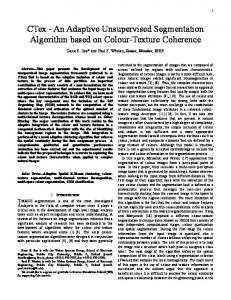
We consider the triple-junction inpainting benchmark introduced by Chambolle and Pock [18]. Figure 1a shows the initial data u0 with the region to be inpainted in gray. The known optimal solution is shown in Fig. 1b, three regions of different colors meeting at a triple junction with an angle of 2π/3. We use the relaxed continuous Potts model with the following data-fidelity term:  El (x) = (u0 (x) − βcl )2 , c={R,G,B}

where {β l := [βRl , βGl , βRl ]T }l=1,...,3 is a vector of predefined colors. In this example we set them to the ground truth. We observe that the sole parameter of ASB influences the convergence behavior of the algorithm. For a large step size γ we observe premature convergence on energy levels higher than the PD reference, resulting in a less binary mask (cf. Figs. 1c and f). For a smaller step size the final energy reached by ASB at iteration n = 104 is comparable (γ = 5) or better (γ = 0.1) than PD (cf. Fig. 1f). Nevertheless, the convergence behavior differs: for the intermediate step size (γ = 5), ASB is initially faster and then slows down compared to PD. For the smaller step size (γ = 0.1), ASB is initially slower than PD, but then reaches lower energy levels quickly. The final masks of these two cases, however, are visually indistinguishable from the mask obtained by PD (cf. Fig. 1e). B. Natural Scenes Segmentation We demonstrate the applicability of our algorithm to natural scene images from the Berkeley database [26]. We use the same energy model as in the previous subsection, except that the L color vectors are now estimated from the data using

a)

b)

Relative Energy

E n −E  E

10

c)

d)

e)

2

a)

b)

L = 5 Δr E = 8.1e−3

c)

d)

L = 5 Δr E = 3.8e−4

e)

f)

L = 5 Δr E = −3.2e−4

g)

h)

L = 6 Δr E = −1.0e−2

10−2

10−6 Primal Dual ASB γ = 0.1 ASB γ = 5.0 ASB γ = 250

10−10 100

f)

101

102

103

104

Iteration number n

Fig. 1. Triple-junction inpainting benchmark. (a) The data image with the grey region to be inpainted. (b) The ground truth solution. All experiments are done with a regularization parameter λ = 1/5. (c) The final mask obtained by the ASB algorithm for γ = 250. (d) The final mask from the primal– dual algorithm and ASB for γ = 0.1 and γ = 5. Only one mask is shown because the three are visually indiscernible. (e) The segmentation obtained after applying the “arg max” rule. It is the same for all cases. (f) The log − log trace of the energy E normalized by the best energy E  obtained among all experiments.

a k-means algorithm. Figure 2 shows the original images and the segmentations obtained by ASB after 500 iterations. We do not show the results obtained by PD as they are visually indistinguishable from the ASB ones. Nevertheless, we indicate their relative energy differences and observe that they are small. For all images the final masks are almost everywhere binary, indicating that the solutions obtained from the relaxed continuous Potts model are in these examples close to the global solution of the original non-convex model. C. Biological Image Segmentation We exemplify a biological application by segmenting a confocal microscopy image of a mammalian cell with fluorescently labelled endosomes (Fig. 3a). To accommodate for the Poisson statistics inherent to such low-intensity microscopy techniques, we use a Poisson negative-log-likelihood datafidelity term. We set the regularization parameter to λ = 0.15 and the step size to γ = 10. The ASB algorithm is stopped when the relative change in the primal energy (Eq. (6)) is below machine precision. The intensity values are estimated by k-means with L = 5 regions. The resulting masks capture the background (Fig. 3c), the cytoplasm (Fig. 3d), and the endosomes (Fig. 3e). The endosomes are divided into three masks according to their different brightness (Fig. 3f1–f3). IV. D ISCUSSION AND C ONCLUSION We followed the idea of Goldstein et al. [15] in applying the alternating split Bregman (ASB) algorithm to image segmentation. We extended their work to the multi-region case

429

Fig. 2. Natural scene segmentation. The first column (a, c, e, g) shows the input images. The second column (b, d, f, h) shows the final masks obtained from the PD and ASB algorithms. The masks from the two algorithms are visually indiscernible and only one is shown. The regularization parameter is set to λ = 1/5 and the step size for ASB is γ = 5. We also show below each segmentation the number of regions L used and the relative difference in energy between the two algorithms defined as Δr E = (EASB − EPD )/EPD .

a)

b)

c)

d)

e)

f1)

f2)

f3)

Fig. 3. Segmentation of fluorescently labelled endosomes. (a) Inverted fluorescence microscopy image corrected for the background using a top-hat filter. (b) The reconstructed inverted image with L = 5 regions. (c–f) The soft membership functions for increasing fluorescence intensity levels: (c) The mask corresponding to the image background; (d) The mask capturing the cytoplasmic compartment; (e) The sum of the remaining three masks capturing the endosomes. (f1–f3) The three endosome masks individually.

by introducing an ASB-based algorithm for solving a large class of convex relaxations of the continuous Potts model using a splitting proposed by Setzer et al. [16]. This results in an efficient decoupling of the different energy terms. The resulting optimization problem decomposes into one leastsquare problem and several independent proximal mapping problems (the w-subproblems). Most of the subproblems can be solved exactly, either analytically or numerically. We have demonstrated the potential of the algorithm on synthetic test cases and real-world images, using the primal–dual (PD) approach of Chambolle and Pock [25] as a benchmark. The results show that our approach compares well with the theoretically well-grounded PD algorithm. The results also suggest that an adaptive strategy for the only parameter of the algorithm could lead to better performance. Moreover, the theoretical understanding of the ASB algorithm should be improved, e.g., by exploring connections between ASB algorithms and other well-known algorithms [27], [21]. From a modeling point of view, one can accommodate other energy terms such as the label-cost prior of Yuan and Boykov [28] and Delong et al. [29]. The ease of adding an additional energy term mainly depends on the ability to solve the associated proximal problem (i.e., the w−subproblem). ACKNOWLEDGMENT The authors thank Prof. Urs Greber (University of Zurich) and Dr. Christoph Burckhardt (Harvard University) for kindly providing the endosome example image. J.C. and G.P. were funded through CTI grant 9325.2-PFLS-LS from the Swiss Federal Commission for Technology and Innovation (to I.F.S. in collaboration with Bitplane, Inc). This project was further supported with grants from the Swiss SystemsX.ch initiative, grants LipidX and WingX, to I.F.S. R EFERENCES [1] D. Mumford and J. Shah, “Optimal approximations by piecewise smooth functions and associated variational problems,” Communications on Pure and Applied Mathematics, vol. 42, no. 5, pp. 577–685, 1989. [2] T. F. Chan and L. Vese, “Active contours without edges,” Image Processing, IEEE Transactions on, vol. 10, no. 2, pp. 266 –277, feb 2001. [3] D. Cremers, M. Rousson, and R. Deriche, “A review of statistical approaches to level set segmentation: Integrating color, texture, motion and shape,” International Journal of Computer Vision, vol. 72, pp. 195– 215, 2007. [4] T. Pock, T. Schoenemann, G. Graber, H. Bischof, and D. Cremers, “A convex formulation of continuous multi-label problems,” in Computer Vision, 2008. ICCV 2008. IEEE 12th International Conference on. Springer Berlin / Heidelberg, 2008, vol. 5304, pp. 792–805. [5] C. Zach, D. Gallup, J.-M. Frahm, and M. Niethammer, “Fast global labeling for real-time stereo using multiple plane sweeps,” in VMV, 2008, pp. 243–252. [6] Y. Boykov, O. Veksler, and R. Zabih, “Fast approximate energy minimization via graph cuts,” Pattern Analysis and Machine Intelligence, IEEE Transactions on, vol. 23, no. 11, pp. 1222–1239, 2001. [7] T. F. Chan, S. Esedo¯glu, and M. Nikolova, “Algorithms for finding global minimizers of image segmentation and denoising models,” SIAM Journal on Applied Mathematics, vol. 66, no. 5, pp. 1632–1648, 2006.

430

[8] L. A. Vese and T. F. Chan, “A multiphase level set framework for image segmentation using the mumford and shah model,” International Journal of Computer Vision, vol. 50, pp. 271–293, 2002. [9] J. Lellmann, J. Kappes, J. Yuan, F. Becker, and C. Schn¨orr, “Convex multi-class image labeling by simplex-constrained total variation,” in Scale Space and Variational Methods in Computer Vision. Springer Berlin / Heidelberg, 2009, vol. 5567, pp. 150–162. [10] T. Pock, A. Chambolle, D. Cremers, and H. Bischof, “A convex relaxation approach for computing minimal partitions,” in Computer Vision and Pattern Recognition, 2009. CVPR 2009. IEEE Conference on, june 2009, pp. 810 –817. [11] J. Lellmann, F. Becker, and C. Schn¨orr, “Convex optimization for multiclass image labeling with a novel family of total variation based regularizers,” in Computer Vision, 2009 IEEE 12th International Conference on, 29 2009-oct. 2 2009, pp. 646 –653. [12] E. Bae, J. Yuan, and X.-C. Tai, “Global minimization for continuous multiphase partitioning problems using a dual approach,” International Journal of Computer Vision, vol. 92, no. 1, pp. 112–129, 2011. [13] E. S. Brown, T. F. Chan, and X. Bresson, “A convex approach for multiphase piecewise constant mumford-shah image segmentation,” UCLA, Tech. Rep. CAM 09-66, 2010. [14] T. Goldstein and S. Osher, “The split bregman method for l1-regularized problems,” SIAM Journal on Imaging Sciences, vol. 2, no. 2, pp. 323– 343, 2009. [15] T. Goldstein, X. Bresson, and S. Osher, “Geometric applications of the split bregman method: Segmentation and surface reconstruction,” Journal of Scientific Computing, vol. 45, pp. 272–293, 2010. [16] S. Setzer, G. Steidl, and T. Teuber, “Deblurring poissonian images by split bregman techniques,” Journal of Visual Communication and Image Representation, vol. 21, no. 3, pp. 193 – 199, 2010. [17] A. Chambolle, V. Caselles, D. Cremers, M. Novaga, and T. Pock, An Introduction to Total Variation for Image Analysis. DE GRUYTER, 2010, vol. Volume 9. [18] A. Chambolle and T. Pock, “A convex approach for computing minimal partitions,” CMAP, Ecole Polytechnique, France, Tech. Rep. 649, 2008. [19] J. Lellmann and C. Schn¨orr, “Regularizers for vector-valued data and labeling problems in image processing,” Control Systems and Computers, vol. 2, pp. 43–54, 2011. [20] J. Lellmann and C. Schn¨orr, “Continuous multiclass labeling approaches and algorithms,” Univ. of Heidelberg, Tech. Rep., 2010. [21] S. Setzer, “Operator splittings, bregman methods and frame shrinkage in image processing,” International Journal of Computer Vision, vol. 92, pp. 265–280, 2011. [22] G. Strang, “The discrete cosine transform,” SIAM Review, vol. 41, no. 1, pp. pp. 135–147, 1999. [23] C. Michelot, “A finite algorithm for finding the projection of a point onto the canonical simplex of Rn ,” Journal of Optimization Theory and Applications, vol. 50, pp. 195–200, 1986. [24] J. Duchi, S. Shalev-Shwartz, Y. Singer, and T. Chandra, “Efficient projections onto the l1-ball for learning in high dimensions,” in Proceedings of the 25th international conference on Machine learning. ACM, 2008, pp. 272–279. [25] A. Chambolle and T. Pock, “A first-order primal-dual algorithm for convex problems with applications to imaging,” Journal of Mathematical Imaging and Vision, vol. 40, pp. 120–145, 2011. [26] D. Martin, C. Fowlkes, D. Tal, and J. Malik, “A database of human segmented natural images and its application to evaluating segmentation algorithms and measuring ecological statistics,” in Proc. 8th Int’l Conf. Computer Vision, vol. 2, July 2001, pp. 416–423. [27] E. Esser, “Applications of lagrangian-based alternating direction methods and connections to split bregman,” UCLA Computational and Applied Mathematics, Tech. Rep., 2009. [28] J. Yuan and Y. Boykov, “Tv-based multi-label image segmentation with label cost prior,” in British machine vision conference (BMVC), 2010. [29] A. Delong, A. Osokin, H. Isack, and Y. Boykov, “Fast approximate energy minimization with label costs,” International Journal of Computer Vision, pp. 1–27, 2011.